Light U(1)s in heterotic string models

Thesis submitted in accordance with the requirements of

the University of Liverpool for the degree of Doctor in Philosophy

by

Viraf M. Mehta

We present the construction of heterotic string models built using the free fermionic formulation, and focus on how additionalU(1)s may arise. We motivate an anomaly free combination, U(1)ζ, as a proton lifetime preserving symmetry external to a

left–right symmetric gauge group. This same combination is found to nullify lepton number inU(1)B−L to form a leptophobic combination, also in left–right symmetric

models, which we compare to other leptophobic U(1) combinations constructed in the context of different gauge groups.

We then accommodate U(1)ζ as a proton lifeguard symmetry in an effective

field theory. We present a comparative study of how gauge coupling unification constraints may be satisfied whenSO(10)_×U(1)ζ 6⊂E6 and when theU(1)ζ charges

do have anE6 embedding. We show that without such an embedding, current values of sin2_{θW(MZ) andα}

This thesis contains material that has appeared in the following publications by the author:

• A. E. Faraggi and V. M. Mehta, Proton Stability and Light Z0 Inspired by String Derived Models,Physical Review D 84(2011), 086006,arXiv:1106. 3082[hep-ph].

• A. E. Faraggi and V. M. Mehta, LeptophobicZ0 in Heterotic–String De-rived Models, Physics Letters B 703 (2011), 567, arXiv:1106.5422[hep-ph]. • A. E. Faraggi and V. M. Mehta, Proton Stability, Gauge Coupling

During my time in Liverpool, I’ve had the pleasure of working with and meeting some great friends and colleagues. The memories made here will stay with me forever and I have many people to thank. Firstly, my supervisor, Alon Faraggi, for the ideas and directions from which this work spawned.

A great deal of thanks to John Gracey and Dave Muskett, to who I am hugely indebted and my gratitude to Ian Jack and Thomas Mohaupt for helping me get to this stage, despite the bumpy road along the way. Thank you also to Tim Jones and Steve Downing for the squash games and for letting me win sometimes.

I’d like to thank my friends Owen Vaughan, Gary Soar, Ruofan Liao, Adriano Lo Presti, Elisa Manno, Conor Smyth, Aaron Roberts, Aaron Bundock, Katie Walters, Rob Purdy, Panos Athanasopoulos, Josh Davies, David Errington, Tom`aˇs Jeˇzo, Paul Dempster, Jaclyn Bell and Stephen Jones for making the time spent in Liverpool most enjoyable. I’ll miss coffee time. I am very grateful to my officemate and good friend Dr William Walters; the journey would have been less fun had I endured it with anyone else.

think of no better person to have by my side for its duration.

1 Introduction 1

1.1 Proton Stability . . . 1

1.2 Unification . . . 5

1.3 Low–scale U(1) . . . 6

1.4 Inspiration from strings . . . 9

2 Model Building & Free Fermionic Formulation 14 2.1 Free Fermionic Formulation . . . 15

2.2 Model–building . . . 19

2.3 The NAHE set . . . 21

2.4 Beyond the NAHE set . . . 29

2.5 Light U(1)s . . . 40

2.6 Normalization of U(1)s . . . 49

3 A Leptophobic U(1) from the Heterotic String 54 3.1 Standard–like models . . . 54

3.2 Left–right symmetric models . . . 58

4.2 Superpotentials . . . 68

5 Phenomenological Analysis 77

5.1 Proton Stability Constraints . . . 78 5.2 Gauge Coupling Analysis . . . 81

6 Accommodating U(1)ζ ⊂E6 in heterotic string models 96 6.1 Enhancement to E6 in string models . . . 97 6.2 Embedding U(1)ζ in E6 . . . 99

7 Conclusions 101

Introduction

The recent discovery of the Higgs boson at the LHC [1, 2] lends further credence to the hypothesis that the Standard Model (SM) provides a viable effective parameter-ization of all subatomic interactions. However, there are many observed results that simply cannot be reproduced within this framework. The unification with gravity and the quantization of electromagnetic charges are but two of these unanswerable questions within the framework of the SM. Current energies being explored at the LHC could lead to interesting new physics beyond the Standard Model (BSM).

1.1

Proton Stability

The main aim of this thesis is to provide a viable solution to the problem of proton stability in a class of supersymmetric extensions of the Standard Model originating in the heterotic string, while accommodating other nuances of the SM, e.g. light neutrinos, three generations and a light Higgs. We propose an additional gauge symmetry, external to that of the SM gauge group,SU(3)C×SU(2)L×U(1)Y, that,

of testing BSM physics.

In the SM, accidental global symmetries conserve baryon and lepton number at the renormalizable level. PDMOs may be induced at dimension-6, i.e.

1 Λ2

p

QLQLQLLL, (1.1)

which, from the current bound on the proton lifetime, indicate that the SM is an effective field theory (EFT) below a cutoff, Λp ∼1016GeV.

Many extensions of the SM that have been proposed to address other issues, in particular the hierarchy problem, introduce a cut–off at the TeV scale. Such extensions consequently induce proton decay at an unacceptable rate. For example, in supersymmetric extensions of the SM, operators violating baryon and lepton number are induced at the renormalizable level. These are given by

QLLLdc L,

ucLd c Ld

c L,

(1.2)

where each of the fields represents a chiral supermultiplet. One must then rely on some ad hoc global or discrete symmetries, to forbid the unwanted terms. For example, in the MSSM, R–parity is invoked to forbid these operators. R–parity is a Z2 symmetry of matter states. The charges are given by a linear combination of SM quantum numbers:

QR = (₋1)3(B−L)+2s, (1.3)

stable. When looking for a unified theory, one must also consider the high energy regime,i.e. _O(MPlanck). Attempts have recently been made to deriveR–symmetries

of this type from string models [4–7]. However, it is expected that only local sym-metries survive quantum gravity effects [8] and so in this thesis we do not consider such symmetries. Instead we investigate an alternative appealing proposition for the suppression of PDMOs: the existence of an abelian gauge symmetry beyond that of the SM gauge group. Allowing the SM matter states to be charged under this additional gauge symmetry, we may forbid PDMOs, which are then only induced at the symmetry’s breaking scale. For the extra symmetry to provide adequate suppression of the unwanted terms, it has to exist at a mass scale within reach of contemporary particle accelerators [9, 10].

The simplest abelian extension one may construct to prohibit PDMOs is by gauging baryon minus lepton number, U(1)B−L, which naturally arises in SO(10)

Grand Unified Theories (GUTs). To date, many SO(10)–based models have been constructed following the various symmetry breaking patterns of this rank-5 Lie group, both in the context of a top–down approach, e.g. the heterotic string (see

e.g.[11] and references within) and in a bottom–up field theory construction [12–16] in 4- and 5-dimensions.

Gauged–(B−L) (GBL) in SO(10) has the advantage of being an anomaly free symmetry. That is, as each of the SM generations (plus a right–handed neutrino) is embedded in a singleSO(10) spinorial representation, the 16, the only two U(1) combinations free of gauge and gravitational anomalies are U(1)B−L and U(1)Y

fermionic models of the heterotic string in Standard–like (SL) models [18–20] and in extra dimensional heterotic string models [21]. In [22], it was shown that sufficiently low neutrino masses could not be produced in SL models built in the free fermionic construction.

The requirement of light neutrino masses necessitates that lepton number is broken. In bottom–upSO(10) grand unified models, one can use the 126 represen-tation, which breaks lepton number by two units and leaves an unbroken symmetry, which still forbids the dimension-4 PDMOs. However, the 126 representation, in general, does not arise in perturbative string models [23]. This implies that lepton number is broken by unit–one carrying fields and thus, the dangerous dimension-4 PDMOs are generated. Specifically, inSO(10), these operators are contained in the

164 term,

QLLLdc Lν

c L,

ucLu c Ld

c Lν

c L,

(1.4)

whereνc

L is the SM singlet field, i.e. the CP–conjugate of νL, and gets a vev of the

order of the GUT scale. Additionally, the 164 gives rise to the dimension-5 terms contained in

QLQLQLLL,

uc

LdcLdcLecL,

(1.5)

which are not forbidden by U(1)B−L. It is therefore apparent that gauged baryon

minus lepton number by itself is not sufficient to guarantee proton stability. Other local gauge symmetries, possibly in conjunction withU(1)B−L, are needed to ensure

neutrino masses and forbids PDMOs up to dimension-6. The necessary requirements and conditions for allowing thisU(1) to be light are discussed in Section 1.3.

1.2

Unification

Another remarkable feature of the MSSM, as well as being the minimal extension to the SM that allows for SUSY and thus alleviates the electroweak–Planck hierarchy problem, is that, at one–loop, the SM gauge couplings unify, i.e. extrapolating the current experimental data for α3(MZ), α2(MZ) and α1(MZ)∗, we find unification atMGUT ∼2·1016GeV [26–28].

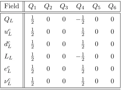
However, as we are constructing a string–inspired model, string–scale unification is expected. In the heterotic string the scale at which coupling unification is pre-dicted isMS ∼5·1017_{GeV [29]. In our analysis we vary the unification scale in this} range, i.e. MGUT ≤ µ≤ MS. We see the effect of this variation on our low–energy

obervables, sin2_{θW (MZ) and α}

3(MZ), in Figure 1.1. As µ moves away from the MSSM unification scale,MGUT, and toward the string scale, MS, we notice that the

values of sin2_{θW (MZ) andα}

3(MZ) move away from their experimental results. The factor of 20 discrepancy between these unification scales was discussed in [30] and it was concluded that intermediate matter thresholds contributed enough to overcome its effect, allowing string unification in a wide class of realistic free fermion heterotic string models. In the analysis of our string–inspired model, we will look to ac-commodate intermediate scales in order for gauge coupling unification at the string scale to occur. It has also been demonstrated that nonperturbative effects arising in heterotic M–theory [31] can push the unification scale down to the MSSM unifi-cation scale [32]. As our additional U(1) will take charge assignments that satisfy

∗_α

heterotic string constraints,i.e. an E8 embedding, we expect a similar model based in the heterotic M–theory regime to have equivalent charge assignments. Thus, al-lowing variation of the unification scale, from MGUT to MS, may also account for

nonperturbative effects.

0.1 0.12 0.14 0.16 0.18 0.2

0.216 0.218 0.22 0.222 0.224 0.226 0.228 0.23 0.232

α3

(

MZ

)

sin2_θ W(MZ)

Figure 1.1: sin2θW(MZ) vs. α3(MZ) with 2·1016.µ.5.27·1017GeV.

The current limits are sin2θW(MZ)

MS= 0.23116±0.00012 andα3(MZ) = 0.1184±0.0007[33].

Hereµruns from right to left.

1.3

Low–scale

U

(1)

Additional abelian spacetime vector bosons beyond those that mediate theSU(3)_×

SU(2)_×U(1)Y subatomic interactions are abundant in extensions of the SM. Their

existence, in both GUTs and string theories, have been amply discussed in the literature [34–36], with the most appealing abelian extensions arising inSO(10) and

E6[37–42]. The embedding of the SM states∗ in three generations of the spinorial16

representation strongly hints at the realisation ofSO(10) in nature, whileE6 GUTs go a step further by accommodating both matter and Higgs states in a common representation, the27. These GUT groups may be reproduced in the heterotic string regime and broken directly to the SM or to subgroups with additional abelian factors [43–46]. A class of three generation heterotic-string models that produce these GUT embeddings are the free fermion models of [18, 19, 47–51], which correspond to compactifications on Z2 × Z2 orbifolds [52–58] due to the relation of bosons and fermions in two dimensions,

ψµ_+iχµ_=:eiXµ

: . (1.6)

This will be the formulation used to discuss our heterotic string models and we review their structure in Chapter 2. The discussion of additional U(1)s in the context of free fermion models has included those that act as proton lifeguards [9, 10, 25, 59] as well as other motivations from potential BSM signatures [60, 61] and supersymmetry breaking [62].

Recently a leptophobic U(1) was motivated due to an excess in the W + 2 jets channel detected at CDF [63]. The absence of such an enhancement in the dilepton channel, as well as constraints arising from direct production at LEPII, TeVatron and LHC searches necessitates suppressed couplings to leptons. This posed an interesting problem as most GUT and string theory models will produce extra bosons with unsuppressed coupling to both leptons and baryons. It is, therefore, of interest to examine how a leptophobicZ0 _{can arise [60, 64]. From a bottom–up approach, one} can simply gauge the baryon number,U(1)B. This exercise has been undertaken [65,

66] and within Type-I string theories a gaugedU(1)Bmay indeed arise. However, in

unsuppressed couplings to leptons.

The abundance of U(1) symmetries in GUTs, and the string models from which they originate, does not necessarily result in their existence at accessible energies. For example, much of the discussion ofU(1) symmetries as proton lifeguards in free fermion models has focussed on the requirements necessary for their existence at the string–scale in addition to accommodating the constraints coming from SM data. These requirements include:

PDMOs – the dimension-4, -5 and -6 proton decay mediating operators must be forbidden;

Light neutrinos – lepton number violation must be allowed in order for a seesaw– mechanism to be realised;

Yukawa couplings – the SM fermions must still form the necessary couplings with the electroweak Higgs doublets in order to generate the correct mass terms upon breaking of SU(2)L×U(1)Y;

Family universal – to avoid flavour changing neutral currents, and to avoid generation– dependent couplings that may induce rapid proton decay, we demand family universality;

Anomaly freedom – to build a consistent effective field theory (EFT) that can describe low–scale physics, while allowing for an additional abelian gauge sym-metry accessible at current experiments, requires the theory to be anomaly free.

ex-istence of the desired symmetry in explicit string constructions guarantees anomaly freedom of the additional U(1), yet facilitating satisfaction of these properties in a phenomenologically viable toy–model can prove to be difficult. In this thesis we construct a string–inspired field theory model that takes into account the ingredi-ents, in particular the string charge assignmingredi-ents, from the string–derived models to explore some phenomenological properties of the extraU(1).

1.4

Inspiration from strings

The models that we use in this thesis are constructed in the free fermionic formu-lation (FFF) of the heterotic string. In the extra–dimensional construction of the heterotic string [67–69], comprising of a supersymmetric left–moving sector and a purely bosonic right–moving sector, it is predicted that there exist ten spacetime dimensions, six of which are compactified on some 6-dimensional manifold, M6_. However, the FFF of the heterotic string is constructed directly in four dimensions, removing the necessity of some geometrical interpretation for the additional dimen-sions. The additional degrees of freedom are thought of as fermions that freely propagate on the string worldsheet, the two–dimensional surface mapped out by the string propagating through time.

directly to an even, self–dual lattice, Γ, which is equivalent to the root lattice of

E8×E8 or the weight lattice of Spin(32)_Z2 .

In extra dimensional models, the additional dimensions are thought to be of microscopic scale (or even Planck), invisible to current detectors. The additional dimensions, though, contain a lot of information that dictates the physics of the four dimensions that we see. This is because in the extra dimensional construction of heterotic string models, the ten–dimensional theory fixes the gauge and matter content. Thus, the description of_M6_{becomes very important in determining unified} string models of particle physics.

However, with the absence of extra dimensions, physics in the FFF of the het-erotic string is not determined by specifying the geometry of additional spacetime dimensions. In fact, to specify models in the FFF, one only requires two ingredients: the phases picked up by the worldsheet fermions; and the generalised GSO phases (see 2.1 and proceeding discussion). Realistic unified string models are, therefore, readily constructed within this framework. Due to their accessibility, one can do vast searches through string vacua [70] with relative ease. New techniques are being adapted for geometrical constructions but for now, comprehensive scans of possible models in string vacua are restricted by our knowledge of_M6 _{geometries [71, 72].}

Outline

In this thesis, we discuss the phenomenological effects of an additional abelian gauge symmetry, external to an SO(10) GUT group. This U(1) is generated by a linear combination of the Cartan generators of the 8-dimensional visible gauge group in the heterotic string construction, and an example is constructed that forbids proton decay mediating operators up to dimension-6 while allowing for light neutrinos via a seesaw mechanism. Another example has suppressed couplings to leptons to form a leptophobic Z0_.

Chapter 2

In this chapter we introduce important concepts with regard to a particular con-struction of the heterotic string: the free fermionic formulation. We give examples of how GUT models are built within this framework and how GUT representations are decomposed under low–scale gauge groups that eventually break to the SM gauge group, SU(3)C ×SU(2)L×U(1)Y. We discuss the string formation of additional U(1)s and motivate two examples: a proton lifeguard combination and a leptopho-bic U(1). We also outline the stringy origins of the matter we will use to build our string–inspired model when constructing a specific model accommodating our proton–protectingU(1).

Chapter 3

a new combination that features in models with the left–right symmetric breaking pattern ofSO(10). The analysis carried out in this chapter featured in [61].

Chapter 4

Here we specify a model whose attributes allow the suppression of proton decay mediating operators up to dimension-6. We build a spectrum, starting with the MSSM, that satisfies the string charge assignments. We present the spectra above and below an intermediateSU(2)R symmetry breaking scale and also the respective

superpotentials. The analysis done in this chapter featured in [73].

Chapter 5

Having specified a model in the previous chapter, we now look at phenomenological constraints that can be applied to our string–inspired model. Specifically we look at how both proton lifetime limits and gauge coupling unification constrain our model. For the GCU analysis, we present a comparison of two classes of models:

SO(10)_×U(1)ζ 6⊂ E6 and SO(10)×U(1)ζ ⊂ E6. This allows us to discuss the benefits and difficulties in each. The analysis done in this chapter featured in [74].

Chapter 6

Chapter 7

To conclude we summarise our results and discuss possible future projects that may extend this work.

Appendix A

In the first appendix, we present the root vectors in the basis we use to construct

SO(10). We use these to build the 16 representation explicitly.

Appendix B

Model Building & Free Fermionic

Formulation

In this review chapter, we present the formalism we use to construct our string models. It treats the extra degrees of freedom, commonly compactified as extra dimensions, as free fermions on the string worldsheet and, thus, these are string models constructed directly in four dimensions. In this section we review the con-struction and structure of the free fermionic formulation; the framework within which we build our models. We then discuss the various semi–realistic gauge groups and matter representations that have been explored in the literature.

From a two–dimensional perspective, bosons and fermions are equivalent, with real fermions and bosons carrying conformal weight 1

2.1

Free Fermionic Formulation

As we are now restricting ourselves to only the four dimensions that have been ob-served in nature, we induce a conformal anomaly on the worldsheet, i.e. the trace over all conformal states in our string theory is now non–zero. This is rectified by including freely propagating fermions as worldsheet degrees of freedom. Requiring a cancellation of the conformal anomaly gives, in the light–cone gauge, 18 worldsheet Majorana–Weyl fermions in the supersymmetric sector and 44 worldsheet Majorana– Weyl fermions in the bosonic sector. We also have the superpartner of the bosonic coordinates in the supersymmetric sector and the bosonic coordinates themselves in both sectors. In the right–moving, bosonic sector, we actually complexify 32 fermionised real degrees of freedom; these 16 complex fermions define our gauge structure. This corresponds to the 16-dimensional internal torus of the compact-ified heterotic string, corresponding to an E8 ×E8 root lattice or Spin(32)_Z

2 weight

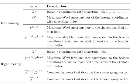
lattice. Due to the non–geometrical interpretation of these models, the additional 12 Majorana–Weyl fermions, bosons corresponding to the compactified dimensions in the bosonic language, allow us to increase the rank of our overall gauge group up to 22. However, as we will see later, these will play the role of a ‘counting’ operator for the number of generations in our semi–realistic models. A full list of worldsheet fields is given in Table 2.1.

All of the physics is contained within the one–loop partition function, i.e. the vacuum–to–vacuum amplitude, and thus gives us access to the full theory,

Z =X

a,b

c

a b

Z

a b

. (2.1)

Label Description

Left–moving

Xµ _{Bosonic coordinates with spacetime index,µ= 0, . . . ,3}

ψµ _{Majorana–Weyl superpartners of the bosonic coordinates}

with spacetime index

χ1,...,6 _{Majorana–Weyl superpartners to the six compactified} di-mensions

y1,...,6_{, w}1,...,6 _{Majorana–Weyl fermions that correspond to the bosons} describing the six compactified dimensions in the bosonic formulation

Right–moving

Xµ Bosonic coordinates with spacetime index

y1,...,6_{, w}1,...,6 _{Majorana–Weyl fermions that correspond to the bosons} describing the six compactified dimensions in the orbifold formulation

ψ1,...,5, η1,2,3 _{Complex fermions that describe the visible gauge sector}

φ1,...,8 Complex fermions that describe the hidden gauge sector

Table 2.1: States that describe our worldsheet, where we have separated the internal freely propagating fermions from the spacetime coordinates. As shown, we have 18 in the left–moving,

supersymmetric sector and 44 in the right–moving, bosonic sector in the light–cone gauge.

vectorsa and b. In fact, along with the generalised GSO (GGSO) coefficients,

c

a b

, (2.2)

we have the tools to describe our models in full. However, as is generic in string model building, one must also take into consideration an overcounting over thespin–

structures i.e. the phases picked up on parallel transport around the loops. In other words, our theory must remain modular invariant. This was considered in [75, 76] and we follow the rules laid out in these papers, known henceforth as theABK rules

Figure 2.1: When parallel transported around either of the two non–contractible loops of the torus, the fermions pick up a phase,α(f), and the bosonic coordinates remain invariant.

loops of the torus,i.e.

f _{→ −}eiπα(f)_{f, α(f)}

∈(₋1,1], (2.3)

where the minus sign is simply convention and f corresponds to our worldsheet fermions. Applying different boundary conditions to each of our fermions will corre-spond to different models in the FFF. These models are generated by a set of basis vectors,bk, describing the transformation properties of the 64 worldsheet fermions

and span a finite additive group

Ξ =

k X

i

nibi (2.4)

'ZNi⊕ · · · ⊕ZNk, (2.5)

where ni = 0, . . . , Ni₋1. In our construction, we will see that this additive set consists of

where the Z2 corresponds to a basis vector with α(f) = 0,1, i.e. antiperiodic or periodic fermions only, and the Z4 a basis vector with some fermions picking up a complex phase,i.e. α(f) = 1

2.

The physical massless states in the Hilbert space of a given sector, α∈Ξ, are then obtained by acting on |0iα with the worldsheet bosonic and fermionic mode

operators, with frequencies νb, νf, νf∗, and by subsequently applying the GGSO

projections,

eiπ(bi·Fα)_−δαc∗

α

bi

|siα = 0 (2.7)

to preserve modular invariance where δα describes the spacetime statistics of the sectorα,i.e.

δα =eiπα(ψµ₎

=±1

(2.8)

i.e. δα = −1 if ψµ _{is periodic in the sector α and thus the state is a spacetime}

fermion, and δα = +1 ifψµ _{is antiperiodic in the sector α, resulting in a spacetime}

boson. Also we have that

(bi·Fα)≡      X real+complex left − X real+complex right     

(bi(f)Fα(f)), (2.9)

whereFα(f) is a fermion number operator counting each mode of f once (and if f

is complex,f∗ _{minus once). All physical states must satisfy the Virasoro condition,}

M2

L =−

1 2+

αL·αL

8 +

X

νL = MR2 =−1 +

αR·αR

8 +

X

νR (2.10)

whereα = (αL_|αR)_∈Ξ and the massless states areM2

L =MR2 = 0.

Thus, the states that are allowed in the Hilbert space are

H=M

α∈Ξ

k Y

i=1

eiπ(bi·Fα) _=δαc∗

α

bi

Those that do not satisfy (2.7) and thus do not appear in_H are said to beprojected

out.

For a sector consisting of periodic complex fermions only, the vacuum is a spinor, |±i, representing the Clifford algebra of the corresponding zero modes, f0 and f0∗,

which have fermion number F(f) = 0,−1 respectively. In addition, the Cartan subalgebra of our rank–22 group isU(1)22_{, generated by the right–moving currents,}

f f∗. For each complex fermion, f, theU(1) charges correspond to

Q(f) = 1

2α(f) +F(f). (2.12)

The representation (2.12) shows thatQ(f) is identical with the worldsheet fermion numbers, F(f), for worldsheet fermions with Neveu–Schwarz boundary conditions,

α(f) = 0, and is F(f) + 1

2 for those with Ramond boundary conditions, α(f) = 1. The charges for the |±ispinor vacua are ±1

2.

2.2

Model–building

As we are building our string models within the heterotic string regime, we will now discuss the correspondence between the standard compactification methods used and their description in the FFF.

of E8×E8 or the weight lattice of Spin(32)_Z2 as first demonstrated in [67–69].

In the FFF of the heterotic string, the gauge structure can be described by any of the right–moving free fermions, in general. In fact, the simplest case is that all 44 fermions are periodic. Allowing the left–movers to also remain invariant under parallel transport aroundaandb forms a 64-vector with all the worldsheet fermions being periodic. This is known as the1vector and generates anSO(44) gauge group, the starting point of all NAHE–based models. As shown in Appendix B and [75–77], models built in the FFF all begin with the 1 vector. Below we will briefly discuss the construction of the NAHE set [78], focussing on the visible gauge and matter sectors. As our main aim is to explore specific models rather than generalities in the construction, we specify our gauge structure to be described by sixteen complex right–moving fermions,ψ1,...,5, η1,2,3_{, φ}1,...,8_{, where:}

• φ1,···,8 generate the rank eight hidden gauge group;

• ψ1,···,5 generate theSO(10) GUT gauge group;

• η1,2,3 _{generate the three remaining U(1) generators in the Cartan subalgebra} of the observable rank eight gauge group.

A combination of these three U(1) currents plays the role of the proton lifeguard [73] and a linear combination of these will also be shown to cancel the lepton num-ber component of U(1)B−L such that an effective baryon number gauge symmetry

2.3

The NAHE set

There are two broad classes of free fermionic models that have been studied in the literature: the first are models that utilise the NAHE set of boundary condition basis vectors, which we discuss here; the second are the models spanned in the classification of [57, 79, 80]. The two classes differ in that the first allows and uses complexified internal fermions from the set_{y, w_|y, w_}, resulting in additional

U(1) gauge symmetries, whereas such fermions have not been incorporated in the second class to date. The treatment of the sixteen complex worldsheet fermions that generate the gauge degrees of freedom is identical in the two classes of models. As both the extra proton safeguarding U(1) and the leptophobic U(1) symmetry arise exclusively from these worldsheet fermions, the two classes are identical in respect to the extraU(1)s of interest here. To date, the majority of phenomenological studies of free fermionic models are NAHE–based [78] with the notable exception being the exophobic∗ _{Pati–Salam vacua of [81–83]. For definiteness, we discuss the NAHE–} based models and provide a brief discussion of how the different gauge structures of these models are derived. This will highlight necessary techniques of symmetry breaking/enhancement which will become useful later on. The first stage in the construction of these models consists of the1 vector, mentioned before, where,

1=nψµ, χ1,...,6, y1,...,6, w1,...,6|y1,...,6, w1,...,6, ψ1,...,5, η1,2,3, φ1,...,8o. (2.13)

We are using the convention of any fermions present in_{. . ._}transforming trivially under parallel transport and_|separates right–movers, indicated also with bars, from left–movers. In the case of the1vector, the right–moving fermions are

indistinguish-∗_{i.e. models without exotics. Exotics are states that have fractional electromagnetic charge}

able and so generate anSO(2n), wherenis the number of complex fermions. In this casen = 22 and so we have the gauge bosons ofSO(44) originating in the 0–sector, or the NS–sector, i.e.

ψµ_φa_φb_|0i

NS for a, b= 1, . . . ,44. (2.14)

At this stage the spectrum also contains the gravity multiplet, a tachyon and no supersymmetry. The gravity multiplet is actually a model–independent feature and can be shown to be present in all string models built in the FFF, independent of specifying basis vectors.

We then add the vector

S =

ψµ_{, χ}1,...,6 _{. (2.15)}

The S–sector is now also massless and is, in fact, a Ramond vacuum due to the presence of only complex periodic fermions; we may complexify real fermions with equivalent boundary conditions in the spin–structures as

ψµ_{= √}1

2 ψ

1_+iψ2

χ12_{= √}1 2 χ

1 _+iχ2

χ34 _{= √}1 2 χ

3_+iχ4

χ56 _{= √}1 2 χ

5_+iχ6

(2.16)

or their conjugatesλ∗ab _{= √}1 2 λ

a_−iλb

. As mentioned previously these carry U(1) charge, _±1

2, and so we introduce a combinatorial notation

4 0

+_{· · ·}+

4 4

(2.17)

where the combinatorial factor counts the number of_|−iin the degenerate vacuum of a given state. Our GGSO projection c

1

S

even (+1) number of _|−i. Our choice is even, i.e. c

1

S

= +1. The S–sector contains the gravitini,

4 even

∂Xµ_|0_iS, (2.18a)

and the gaugini,

4 even

φaφb_|0_iS, (2.18b)

of our spectrum and we see that we have_N = 4 spacetime SUSY. As of yet, neither of our sectors,0 or S, contain matter states.

2.3.1

Adding b

To complete the NAHE set, we add the basis vectorsb1,b2 and b3,

b1 =

n

ψµ_{, χ}12_{, y}3,...,6_|y3,...,6_{, ψ}1,...,5_{, η}1o_{, (2.19a)}

b2 =

n

ψµ_{, χ}34_{, y}1,2_{, w}5,6

|y1,2_{, w}5,6_{, ψ}1,...,5_{, η}2o_{, (2.19b)}

b3 =

n

ψµ_{, χ}56_{, w}1,...,4

|w1,...,4_{, ψ}1,...,5_{, η}3o_{. (2.19c)}

These act in similar fashion and so it will be demonstrative to explore one of these, say b1, in more detail and simply show the highlights of the other two. We first consider how this acts on our gauge bosons in the0–sector. From (2.8) we see that

δb1 =−1. (2.20)

This implies that for a state to survive the GGSO projections, pairs of internal fermions forming bosonic states withψµ _{in the NS–sector must satisfy,}

As we can see, the states that survive and correspond to gauge bosons are

ψµn_y3,...,6_{, ψ}1,...,5_{, η}1o n_y3,...,6_{, ψ}1,...,5_{, η}1o

|0_{iNS '} SO(16); (2.22a)

ψµn_y1,2_{, w}1,...,6_{, η}2,3_{, φ}1,...,8o n_y1,2_{, w}1,...,6_{, η}2,3_{, φ}1,...,8o

|0_{iNS '} SO(28). (2.22b)

Therefore our gauge group has broken from

SO(44) →SO(16)×SO(28). (2.23)

In the S–sector, we find that two of our gravitini are projected out,

4 1 + 4 3

∂Xµ|0iS →

2 1

| {z } ψµ_{, χ}12

2 0 + 2 2

| {z }

χ34_{, χ}56

∂Xµ|0iS,

(2.24)

resulting in_N = 4_{→ N} = 2 spacetime SUSY. We also have four generations of the

128spinor representation ofSO(16) coming from the b1–sector: the vacuum of the

b1 sector is Ramond, i.e. a degenerate|±i, and so we have

12 0 +· · ·+ 12 12 , (2.25)

i.e. 4096 states. The GGSO projection, c

1

b1

is chosen such that only the even states remain, i.e.

12 even

= 2048 states. (2.26)

This can be decomposed into the 128 and 128 of SO(16) as

2 0 + 2 2

| {z }

ψµ_,χ12

2 0 + 2 2

| {z }

y3,...,6

8 even

| {z }

y3,...,6_,ψ1,...,5_,η1

where

8 even

'128 (2.28a)

and

8 odd

'128. (2.28b)

As stated, we have four generations of each representation coming from the b1– sector. In the (b1+S)–sector we have the superpartners of these states. In fact,

S is our SUSY generator, thus any states that appear in the sector α will have superpartners inα+S.

We will now see how this decomposes under b2 and b3, along with the gauge bosons in the NS–sector.

2.3.2

Addition of b

and b

We will find that addingb2 andb3 results in the gauge groupSO(10)×SO(6)3×E80 with _N = 1 spacetime SUSY and that the vacuum contains forty–eight multiplets in the16 chiral representation of SO(10), sixteen coming from each of b1,b2,b3.

Gauge bosons At the level of _{1,S,b1}, we had the gauge bosons in (2.22) gen-eratingSO(16)_×SO(28), with 4 generations of the 128 and 128 of SO(16)∗_{. We} also had N = 2 SUSY. Adding b2 in the NS sector decomposes the SO(16) gauge bosons as,

ψµ

y3,...,6_{, η}1

y3,...,6_{, η}1

|0_{iNS '}SO(6)1, (2.29a)

ψµn_ψ1,...,5o n_ψ1,...,5o

|0_{iNS '}SO(10), (2.29b)

∗_{As well as our spinor representations, we have scalars that transform under both gauge groups.}

i.e. SO(16) _→ SO(10)_× SO(6)1. In a similar fashion, the SO(28) is broken to

SO(22)_×SO(6)2, with the generating bosons,

ψµ

y1,2_{, w}5,6_{, η}2

y1,2_{, w}5,6_{, η}2

|0_iNS'SO(6)2, (2.30a)

ψµn_w1,...,4_{, η}3_{, φ}1,...,8o n_w1,...,4_{, η}3_{, φ}1,...,8o

|0_iNS'SO(22). (2.30b)

Theb3 then splits the{w1,...,4, η3}and the

n

φ1,...,8oresulting inSO(22)_→SO(6)3×

SO(16)0_{. TheSO(6)}

i are flavour symmetries as the different generations are charged

under each different SO(6). We will see that our proton lifetime preserving U(1) will originate in these and that we may form a linear combination that is family universal,

U(1)ζ =U(1)1+U(1)2 +U(1)3 (2.31)

The sector,ξ, formed by the combination

ξ =1+b1+b2+b3 ≡

φ1,...,8 _{, (2.32)}

generates

8 even

'128. (2.33)

However, unlike the b1–sector, the massless states of ξ in the left–moving sector are not degenerate; they are obtained by acting on the vacuum with a fermionic oscillator. Therefore,

ψµ

8 even

|0_iξ (2.34)

and

SO(10)×SO(6)3×E80 (2.35)

is the overall gauge group at the level of the NAHE set.

Chiral Matter Earlier we saw that we have four generations of the 128and 128

of SO(16) originating in b1, at the level of the set {1,S,b1}. With the addition of

b2, we must now decompose as SO(10)×SO(6)1 representations. Considering the GGSO projections, c 1 b1 =c 1 b2

=₋1, (2.36)

we find that (2.27) decomposes as

ψµ_,χ12

z }| {

2 0

y3,...,6_|y3,...,6

z }| {

4 even

ψ1,...,5

z }| {

5 even + 2 2 4 odd 5 odd η1

z }| { 1 0 (2.37a) + 2 2 4 even 5 odd + 2 0 4 odd 5 even 1 1 (2.37b) where 5 even

'16 (2.38)

with 5 0 (2.39)

being the highest weight. Also,

5 odd

with

5 5

(2.41)

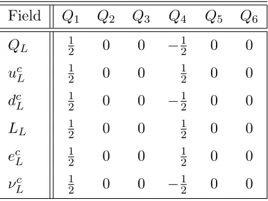
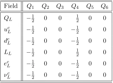
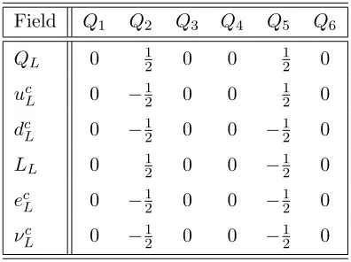
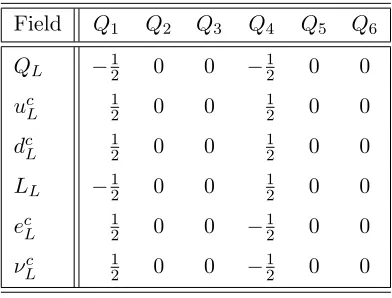
the highest weight in this case. We explicitly construct the16representation in this basis in Appendix A. For b2 and b3, the corresponding fermions are 4 = _{y1_y2_{, w}5_w6_{, y}1_y2_{, w}5_w6_{}, 2 = {ψ}µ_{, χ}34_{}, 5 = {ψ}1,...,5_{} and 1 = {η}2_{} and} 4 = {w1,...,4_{, w}1,...,4_{}, 2 = {ψ}µ_{, χ}56_{}, 5 = {ψ}1,...,5_{} and 1 = {η}3_{} respectively and} so we have a total of 48 generations of the16 and 16 representations, sixteen com-ing from each of thebi–sectors. As we can see, the multiplicative factor determining

the number of 16s comes from the boundary conditions on

yi_{, w}i

|yi_{, w}i _{. (2.42)}

This was discussed in depth in [84, 85]. We also notice that, at the level of the NAHE set, half the generations per bi carry charge of the opposite sign to the

other half of the16 representations under theU(1) combination, (2.31). As we will see, upon breaking SO(10) using further basis–vectors at the string scale, we are able to project out half the states of each representation resulting in a complete representation being formed by states withQζ of opposite sign. This is dependent on the symmetry breaking pattern down from SO(10) and our choices of GGSO projections, as outlined in the next section. The GGSO projections that we have used for the NAHE set are summarised as:

1 S b1 b2 b3



      



      

1 1 1 −1 −1 −1

S 1 1 1 1 1

b1 −1 −1 −1 −1 −1

b2 −1 −1 −1 −1 −1

b3 −1 −1 −1 −1 −1

2.4

Beyond the NAHE set

The second stage consists of adding three or four basis vectors, typically denoted by{α, β, γ}, to the NAHE set. The additional basis vectors reduce the number of generations to three and break the four dimensional gauge symmetry. In this section we explore the various patterns ofSO(10) breaking and how they are realised in the FFF. We also look at how the matter representations are decomposed for our various symmetry breaking patterns.

2.4.1

Visible Gauge–Symmetry Breaking Patterns

At the level of the NAHE set, the GUT group in the visible sector is SO(10), generated by the worldsheet fermions ψ1,...,5. Assigning different boundary condi-tions to these fermions, in a way consistent with the string constraints outlined in Appendix B, leads to various symmetry breaking patterns at the string scale,

MS. We will outline those commonly seen in semi–realistic free fermionic models below. When breaking to the maximal subgroups, the flipped SU(5) (FSU5) and Pati–Salam (PS) breaking patterns, we use a single basis vector to break SO(10) at the string scale. However, we may also employ more than one basis vector to break the GUT group further at MS, removing the need for an intermediate GUT scale, MGUT; the standard–like (SL) and left–right symmetric (LRS) models being

the most commonly seen in the literature [18, 19, 51].

Flipped SU(5)

In order to breakSO(10)_→SU(5)_×U(1) we take

αnψ1,...,5o=

1 2 1 2

1 2 1 2 1 2

. (2.44)

Assumingδα =−1⇔α(ψµ_{) = 1, we require the}

ψ ψ pairs to satisfy

α_·FNS = 0 mod 2 (2.45)

in order for the states to survive the GGSO projection. Therefore, the only combi-nations permitted are

ψµψi∗ψj|0iNS (2.46a)

ψµ_ψi_ψj∗_|0i

NS. (2.46b)

We can easily see that we now have 25 generators: 20 for i 6= j and 5 Cartan generators, wherei=j. Thus we have a rank–5, dimension–25 group, i.e.

U(5)_'SU(5)_×U(1). (2.47)

The FSU5 models were first constructed in string–models in [48, 78, 86] and further phenomenological analysis was done in [87, 88].

Pati–Salam

To breakSO(10)_→SO(6)_×SO(4) makes use of only periodic boundary conditions for the SO(10) generators, i.e. Z2 boundary conditions,

αnψ1,...,5o={11100}. (2.48)

Again assuming δα = ₋1_⇔ α(ψµ_{) = 1, we require (2.45) to hold for the}

ψ ψ

pairs and so only

for i, j = 1,2,3 or i, j = 4,5 survive. The GGSO projections remove 24 generators from our spectrum and we are only left with 21: 15 originating from i, j = 1,2,3 and 6 from i, j = 4,5. Therefore, our gauge group is now a product of a rank– 3, dimension–15 group, i.e. SO(6) ' SU(4), and a rank–2, dimension–6 group,

i.e. SO(4)'SU(2)×SU(2), and so the resulting breaking is

SO(10)−→α SU(4)×SU(2)×SU(2). (2.50)

Standard–like

Here we apply both breaking patterns demonstrated above in two separate basis vectors,

αnψ1,...,5o=

1 2

1 2

1 2

1 2

1 2

(2.51a)

βnψ1,...,5o=_{11100_}. (2.51b)

As we saw previously, following the application of α, 25 generators remain:

i6=j 

 

 

ψµ_ψi∗_ψj_|0i

NS

ψµ_ψi_ψj∗_|0i

NS



 

 

20 generators, (2.52a)

i=j{ψµψi∗ψj|0iNS} 5 Cartan generators. (2.52b)

Applyingβ projects out 12 gauge bosons and only the combinationsi, j = 1,2,3 and

i, j = 4,5 survive. Thus, the product of a rank–3, dimension–9 group, i.e. U(3) _'

SU(3)_×U(1), and a rank–2, dimension–4 group,i.e. U(2)_'SU(2)_×U(1), remain. Our symmetry breaking pattern at the string–scale is

Left–right Symmetric

Similarly, we can break SO(10) → SU(3) ×SU(2)×SU(2) by the application of two basis vectors,

αnψ1,...,5o=_{11100_} (2.54a)

βnψ1,...,5o=

1 2

1 2 1 200

. (2.54b)

The application ofαto the NS sector of the NAHE set gives, as was shown previously, the PS gauge group,i.e.SO(6)×SO(4). Applyingβ projects out 6 generators from the 15 that generate SO(6) and leaves the SO(4) untouched. We are now left with a rank–3, dimension–9 group,i.e. U(3), as seen earlier. Therefore our visible gauge group at the string–scale is

SO(10) _−−→α,β SU(3)_×U(1)_×SU(2)_×SU(2). (2.55)

SU(4)×SU(2)×U(1)

Alternatively, we can instead assign ψ4,5 complex boundary conditions,i.e.

βnψ1,...,5o=

0001 2

1 2

. (2.56)

This would result in

SO(10)−−→α,β SU(4)×SU(2)×U(1) (2.57)

as 2 gauge bosons would be projected out from the 6 that generateSO(4). Here the

SO(6) generators remain untouched.

2.4.2

Matter

So far, viable three generation models withSU(5)×U(1) [78], SO(6)×SO(4) [49, 50], SU(3)_×SU(2)_×U(1)2 _{[18–20], or SU(3)×SU(2)}2 _{×U(1) [51, 90], SO(10)} subgroups have been constructed. Three chiral generations arise from the sectorsb1,

b2 andb3, and are decomposed under the finalSO(10) subgroup below. The flavour

SO(6)3 _{groups are broken to products of U(1)}n _{with 3 ≤ n ≤ 9. This comes from}

assigning different boundary conditions to{y3,...,6_|y3,...,6_}inb

1,{y1,2, w5,6|y1,2, w5,6} in b2 and {w1,...,4|w1,...,4} in b3, than to our right–moving complex fermions ηi in

bi, which generate theU(1)1,2,3 factors.

Above, we have shown the origin of the 16 representation of SO(10) in free fermion models. Here we present how these are decomposed under the various subgroups.

FSU5 BreakingSO(10)_→SU(5)_×U(1) decomposes the16 as

16_→15+101+5−3, (2.58)

corresponding to

5 0

+

5 2

+

5 4

→

5 0

| {z }

15

+

5 2

| {z }

101

+

5 4

| {z }

5−3

,

(2.59)

5 0 → 3 0 2 0

| {z }

ec , (2.60a) 5 2 → 3 2 2 0

| {z }

dc + 3 1 2 1

| {z }

QL + 3 0 2 2

| {z }

νc , (2.60b) 5 4 → 3 2 2 2

| {z }

uc + 3 3 2 1

| {z }

LL

, (2.60c)

with

Y = 1

3Tr [U(3)C] + 1

2Tr [U(2)L], (2.61)

where

Tr [U(3)C] =

3

2(B −L)≡QC (2.62)

and

Tr [U(2)L] = 2T3R ≡QL. (2.63)

This combination is a universal combination for NAHE–based models. Before break-ing to the SM, the FSU5 model may also go via an intermediate breakbreak-ing at the string scale,

SU(5)_×U(1)_→U(3)C×U(2)L →SU(3)C×SU(2)L×U(1)Y (2.64)

PS Writing our 16 in combinatorial notation, decomposed under the PS gauge group,

SO(6)×SO(4)'SU(4)C ×SU(2)L×SU(2)R. (2.65)

we have 5 0 + 5 2 + 5 4 → FL

z }| {

3 1 + 3 3 2 1 (2.66a) + 3 2 + 3 0 2 2 + 2 0

| {z }

FR

(2.66b)

i.e. 16 _→(4,2,1) + 4,1,2. This will break to the SM states via the LRS gauge group

SU(4)C ×SU(2)R×SU(2)L →SU(3)C×SU(2)R×SU(2)L×U(1)C (2.67)

as 3 1 + 3 3 2 1 → QL

z }| {

3 1 2 1 + LL

z }| {

3 3 2 1 , (2.68a) 3 2 + 3 0 2 2 + 2 0 → QR

z }| {

3 2 2 2 + 2 0 + 3 0 2 2 + 2 0 ,

| {z }

LR

where (2.68b) then decomposes to the SM states,

QR∼

3,2,1,₋1

2, 1 2 → uc L

z }| {

3,1,₋2

3

+

dc L

z }| {

3,1,1

3

, (2.69a)

LR∼

1,2,1,3

2, 1 2

→(1,1,0)

| {z }

νc L

+ (1,1,1)

| {z }

ec L

. (2.69b)

The breaking ofSO(10)→SU(3)C×SU(2)L×SU(2)R×U(1)C is via the PS gauge

group, and it is clear from (2.66), the states in FL and FR must have charges of

opposite sign under theU(1)ζ combination in (2.31), whereas breaking SO(10) via

FSU5 does not give these charge assignments. In fact, taking this route of symmetry breaking pattern restricts the charge of all the states in the 16 to be of the same sign as either (2.37a) or (2.37b) are projected out.

In order to elucidate theU(1)1,2,3charges of the matter states in the free fermionic models, it is instructive to extend theSO(10) symmetry, at the level of the NAHE set, toE6. This is achieved by adding to the NAHE set the basis vector [91, 92],

x_≡

n

ψ1,···,5, η1,2,3o. (2.70)

2.4.3

Addition of x

As there are 8 periodic right–moving complex fermions, the vacua in the x-sector are degenerate,|±i. Thus, before the GGSO projections, we have 256 states,

8 0 +· · ·+ 8 8 . (2.71)

Once we apply the GGSO projections

c x 1 =c x S

half of these states are projected out. We are therefore left with either 8 even (2.73a) or 8 odd . (2.73b)

For our choice of GGSO,

c x 1 =c x S

=₋1 (2.74)

we keep (2.73a). As we saw earlier, the NS-sector contains the gauge bosons that generate

SO(10)×U(1)3×SO(16)0 (2.75)

and the gauge bosons in the ξ-sector enhance the hidden SO(16)0 →E80.

The gauge bosons coming from the x-sector transform as the 16 and 16 of

SO(10),

ψ1,...,5

z }| {

5 even

η1,2,3

z }| {

1 0 1 0 1 0 + 5 odd 1 1 1 1 1 1 , (2.76)

and enhance the SO(10) _× U(1) _→ E6 where the U(1) combination is given by (2.31). Adding the x basis–vector at the level of the NAHE set, the gauge group is enhanced to SO(4)3_×E

previously, and the sectors (bi+x) produce the vectorial (10+1)+1representations

in the decomposition of the27 representation of E6

27=16_±1

2 +10∓1+1±2 (2.77)

underSO(10)×U(1). The additional “1” arising in the (bi+x) sectors is an E6 sin-glet. These are obtained by acting on the vacuum with the oscillators of the complex worldsheet fermionsnψ1,...,5ηio_{, which have Neveu–Schwarz boundary conditions in}

the sectors bi+x.

The vacuum of the sectorsbicontain twelve periodic fermions, with each periodic

fermion giving rise to a two dimensional degenerate vacuum_|+_iand_|−iwith fermion numbers 0 and₋1, respectively. After applying the GGSO projections, we can write the degenerate vacuum of the sectorb1 in combinatorial form:

4 0 + 4 2 + 4 4 2 0 5 0 + 5 2 + 5 4 1 0 (2.78a) + 2 2 5 1 + 5 3 + 5 5 1 1 (2.78b)

where 4 = _{y3_y4_{, y}5_y6_{, y}3,4_{, y}5,6_{}, 2 = {ψ}µ_{, χ}12_{}, 5 =} n_ψ1,...,5o _{and 1 = {η}1_{}. We} notice that half of the states from (2.27) are projected out due to our choice of

c

x b1

=−1 (2.79)

The charge under the U(1) symmetry generated by η₁ is determined by its vac-uum state, being a Ramond state in the _|+_i vacuum for the degenerate vacuum in (2.78a). Hence, in this case the U(1)1 charge is +1₂. Similar vacuum struc-ture is obtained for the sectors b2 and b3 with {χ34, y1,2, w5,6|y1,2, w5,6, η2} and {χ56_{, w}1,...,4_|w1,...,4_{, η}3_{} respectively.}

The 10+1 in the 27 of E6 are obtained from the sector bi+x. The effect of

adding the vectorxto the sectors bi is to replace the periodic boundary conditions

for nψ1,...,5, ηio _{with periodic boundary conditions for η}j,k _{with i 6= j 6= k and} i, j, k_{∈ {}1,2,3_}. Consequently, massless states from the sectors bi+x are obtained

by acting on the vacuum with a fermionic oscillator.

If the space–time vector bosons that enhance the SO(10)×U(1) symmetry to

E6 are projected out, either the spinorial 16 or the vectorial (10+1) +1, survive the GGSO projections at a given fixed point. By breaking the degeneracy with respect to the internal fermions {y, w|y, w} we can obtain spinorial and vectorial representations from the twisted sectors at different fixed points. A classification of symmetric free fermionic heterotic string models along these lines was done in [57, 79, 80, 93].

When theSO(10)_×U(1) symmetry is enhanced toE6, the charges of the spinorial

16, the vectorial10and the singlet1, under theU(1)ζ, are fixed by theE6symmetry, as shown in (2.77). When the E6 symmetry is broken by the GGSO projections,

i.e. the x–sector bosons are projected out, the U(1)ζ charges are not restricted by

the E6 embedding, and can take either sign. The U(1) symmetry that serves as the proton lifeguard is a combination of the threeU(1) symmetries generated by the worldsheet complex fermionsη1,2,3_{. The states from each of the sectorsb}

U(1) combination in (2.31) is family universal. This is also true of the leptophobic combination as it is just a linear combination ofU(1)ζ and U(1)B−L.

2.5

Light

U

(1)s

In the string derived models of [18–20, 48, 49, 78], the U(1)1,2,3 are anomalous. Therefore, U(1)ζ ≡ U(1)A is also anomalous and must be broken near the string

scale. In the string derived left–right symmetric models of [51],U(1)1,2,3 are anomaly free and hence the combination U(1)ζ is also anomaly free. It is this property of

these models which allows thisU(1) combination to remain unbroken.

It is instructive to study the characteristics of U(1)ζ in the left–right symmetric

string derived models [51], versus those ofU(1)Ain the string derived models of [19,

49, 78, 94]. We note that both U(1)ζ as well as U(1)A are obtained from the same

combination of complex right–moving worldsheet currents η1,2,3_{. The distinction} between the two cases, as we describe below, is due to the charges of the SM states, arising from the sectors b1, b2 and b3, under this combination.

The periodic boundary conditions of the worldsheet fermionsηi _{ensures that the}

fermions from each sectorbiare charged with respect to one of theU(1)isymmetries.

In the models of [18–20, 48, 49, 78] the charges of a givenbi generation underU(1)i is

chirality in the two terms of (2.66). The reason being that the combinatorial factor with respect to ψ1,...,3 is odd in the first term and even in the second, with the

γ projection that utilises (2.48) being blind to ψ4,5. On the other hand, in the models that utilise (2.44), the γ projection is not blind to ψ4,5, and consequently, the vacuum of ηi _{is fixed with the same chirality for all the states arising from the}

sectorbi.

Thus, in models that descend fromSO(10) via theSU(5)_×U(1) breaking pattern the charges of a generation from a sectorbi, wherei= 1,2,3, under the

correspond-ing symmetry U(1)i, are either +1₂ or −1₂ for all the states from that sector. In

contrast, in the left–right symmetric string models, the corresponding charges, up to a sign, are

Qj(2L) = +1/2; Qj(2R) =−1/2, (2.80)

i.e. the charges of the SU(2)L doublets have the opposite sign from those of the SU(2)R doublets. In fact, this is the reason that, in contrast to the FSU5 and

the SL string models, in the LRS models, the U(1)i symmetries are not part of

the anomalous U(1) symmetry. This arises because the SO(10) symmetry is not enhanced toE6. If the NAHE symmetry is extended to E6, the spinorial 16 states with the “wrong” U(1)ζ charge are projected out, as is the case in the FSU5 and

SL models, as well as the PS models constructed to date.

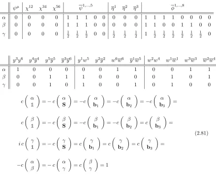
further in this thesis. We refer the interested reader to [51] for the full gauge group of the model, including the hidden sector.

ψµ _χ12 _χ34 _χ56 _ψ1,...,5 _η1 _η2 _η3 _φ1,...,8

α 0 0 0 0 1 1 1 0 0 0 0 0 1 1 1 1 0 0 0 0

β 0 0 0 0 1 1 1 0 0 0 0 0 1 1 0 0 1 1 0 0

γ 0 0 0 0 1 2

1 2

1

2 0 0 1 2 1 2 1 2 1 1 2 1 2 1 2 1 2 1 2 1 2 0

y3_y6 _y4_y4 _y5_y5 _y3_y6 _y1_w5 _y2_y2 _w6_w6 _y1_w5 _w2_w4 _w1_w1 _w3_w3 _w2_w4

α 1 0 0 0 0 0 1 1 0 0 1 1

β 0 0 1 1 1 0 0 0 0 1 0 1

γ 0 0 1 0 1 0 0 1 0 1 0 0

c

α

1

=₋c

α

S

=₋c

α

b1

=₋c

α

b2

=₋c

α b3 = c β 1

=₋c

β

S

=₋c

β

b1

=₋c

β b2 =c β b3 = i c γ 1

=−c

γ S =c γ b1 =c γ b2 =c γ b3 = −c α β =₋c

α γ =c β γ = 1 (2.81)

Table 2.2: LRS Model 1 boundary conditions. Below are the GGSO coefficients, where the GGSO coefficients for the NAHE set were already shown in (2.43). Taken from [51].

2.5.1

Proton Lifeguard

The preservation of theU(1) combination

as an anomaly free symmetry is the key to keeping it as an unbroken low–scale symmetry. The left–right symmetric string models admit cases without any anoma-lous U(1) symmetry; free of any gauge and gravitational anomalies. We note that there may exist string models in the classes of [19, 49, 78, 94] in which U(1)ζ is

anomaly free. This may be the case in the so–called self–dual vacua of spinor vector duality. In [79] a duality symmetry was uncovered in the space of fermionicZ2×Z2 symmetric orbifolds under the exchange of the total number of twisted spinor plus anti–spinor and twisted vector representations ofSO(10). The self–dual models are the models in which the total number of spinors and anti–spinors is equal to the total number of vector representations. The self–dual models are free of any U(1) anomalies. Thus, in such self–dual models with three light chiral generations the

U(1)ζ combination is anomaly free and can remain unbroken below the string scale.

Such quasi–realistic self–dual string models, with an anomaly free U(1)ζ, have not

been constructed to date.

Here, we discuss the stringy origins of the SM matter and additional matter that may be included in our effective theory to allowU(1)ζ to remain anomaly free. In

addition to the three light SM generations arising from the twisted sectors, bi, the

string models contain additional states arising from the twisted or untwisted sectors. The additional spectrum is in general highly model dependent. Later we will fix our string–inspired model by fitting it with additional states that are compatible with the string charge assignments.

The twisted sectors can produce additional states that arise from spinorial rep-resentations of the underlyingSO(10) symmetry with charges_±1

Sectors that contain the basis vectors that break the SO(10) gauge symmetry, generically produce exotic states with fractionalQEM that must obtain a sufficiently

high mass. We note the existence of exophobic heterotic string models in which fractionally charged states appear only in the massive string spectrum [83]. We do not consider these states further here.

As shown previously, the twisted sectorsbi+x produce states that transform in

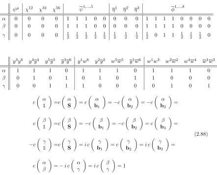
the vectorial representations of the underlying SO(10) GUT symmetry. A twisted sector that produces SO(10) vectorial representations does not exist in the model of Table 2.2. An alternative model that gives rise to twisted states in the vectorial representation ofSO(10) is given in Table 2.3.

The sector b1+b2+α+β in the additive group, Ξ, spanned by this basis gives rise to twisted vectorial SO(10) representations. In this sector, the charges under the

U(1)ζ are fixed by the vacuum of theη1 and η2.

In the left–right symmetric models, the twisted sectorsbi+xproduce states that

transform as SU(2)L×SU(2)R bi-doublets with the U(1)ζ charge assignments

(1,2,2,0,±1) (2.83)

as well as colour triplets. The U(1)ζ charges of these colour triplets is dependent

upon the γ projection and there are several possibilities. If the twisted plane pro-duces bi–doublets with Qζ = +1, then the γ projection dictates that any colour triplet arising from that sector is neutral under U(1)ζ. In this case, we must take

the colour triplets to have the charges

(3,1,1,₋1,0) + 3,1,1,+1,0

(2.84)

ψµ _χ12 _χ34 _χ56 _ψ1,...,5 _η1 _η2 _η3 _φ1,...,8

α 0 0 0 0 1 1 1 0 0 0 0 0 1 1 1 1 0 0 0 0

β 0 0 0 0 1 1 1 0 0 0 0 0 1 1 1 1 0 0 0 0

γ 0 0 0 0 1₂ 1₂ 1₂ 0 0 1_{2 2}1 1₂ 0 1₂ 1₂ 1₂ 1₂ 1₂ 1₂ 0

y3_y6 _y4_y4 _y5_y5 _y3_y6 _y1_w5 _y2_y2 _w6_w6 _y1_w5 _w2_w4 _w1_w1 _w3_w3 _w2_w4

α 1 0 0 0 0 0 1 1 0 0 1 1

β 0 0 1 1 1 0 0 0 0 1 0 1

γ 0 0 1 0 1 0 0 1 0 1 0 0

c

α

1

=₋c

α

S

=₋c

α

b1

=₋c

α

b2

=₋c

α b3 = c β 1

=−c

β

S

=−c

β

b1

=−c

β

b2

=−c

β b3 = i c γ 1

=₋c

γ S =c γ b1 =c γ b2 =c γ b3 = c α β =−c

α γ =c β γ = 1 (2.82)

Table 2.3: LRS Model 2 boundary conditions and GGSO projection coefficients for the additional basis vectors,_{α, β, γ_}, where the GGSO coefficients for the NAHE set were already

shown in (2.43). Taken from [51].

respectively, and vice versa.

An alternative possibility, is that more than one twisted plane produces states in vectorialSO(10) representations. In this case, one plane can produce bi–doublets and a second plane produces the colour triplets. Here, the charges of the twisted colour triplets are not correlated with those of the bi–doublets and we can obtain twisted vectorial colour triplets with charges

(3,1,1,+1,−1) + 3,1,1,−1,+1

(2.85a)

or

(3,1,1,+1,+1) + 3,1,1,₋1,₋1

. (2.85b)

Electroweak Higgs bidoublets may also arise from the untwisted sector. However, in this case the γ GGSO projection dictates that they are neutral underU(1)ζ,

H0 = (1,2,2,0,0) =

Hu

+ Hd

Hu _Hd

−

. (2.86)

The untwisted Higgs bidoublet is the one that forms invariant leading mass terms with the Standard Model matter states, due to the fact that theQLandQRmultiplets

carry opposite U(1)ζ charge.

The string models may also produceSO(10) singlets, which carryU(1)ζ charges.

The singlets can arise from the Neveu–Schwarz untwisted sector and twisted sectors that produce vectorial representations, like the sector b1+b2+α+β. The U(1)ζ

charges are fixed according to the following rules:

In the untwisted sector these states arise by acting on the vacuum with two oscillators, ηi _{and η}j_{. Their U(1)}

ζ charges are fixed by the γ projection according

to the sign ofδγ in (2.7), being zero forδγ = +1i.e. γ(ψµ_{) = 0 and±2 forδγ =−1,}

b1+b2+α+β. The singlets from that sector are obtained by acting on the vacuum with η3_{, or with an oscillator of a real fermion from the set {y w}, which are not} periodic in b1+b2+α+β. The U(1)ζ charges are again fixed by the γ projection.

The γ GGSO projection phase in this sector can be either ±1 or ±i. As we have seen, depending on this GGSO phase and the type of state, the U(1)ζ charges in

this sector can be±2,±1 or zero. Therefore, we can have a combination of singlets with charges +2 and +1, as well as singlets with vanishingU(1)ζ charge.

2.5.2

Leptophobic

U

(1)

At the stage of the NAHE set, the gauge group reads

SO(10)_×SO(6)3 ×E₈0

where the additional basis vectors, {α, β, γ}, break the SO(10) GUT group as de-tailed in Section 2.4. The flavour SO(6)3 _{symmetries are broken to U(1)}3+n _with n = 0,_{· · ·} ,6. The first three, denoted by U(1)i, arise from the world–sheet

cur-rents ηi_ηi∗ _{where i = 1,2,3. These three U(1) symmetries are present in all the}

three generation free fermionic models which use the NAHE set and we saw a linear combination of these form the proton lifetime preservingU(1)ζ. Additional

horizon-tal U(1) symmetries, denoted by U(1)j with j = 4,5, ..., arise by pairing two real

fermions from the sets

y3,...,6 _,

y1,2_{, w}5,6 _,

w1,...,4 _{, (2.87)}