Distributed Source Coding Theory, Algorithms and Applications tqw darksiderg pdf

84 Theobald’s Road, London WC1X 8RR, UK This book is printed on acid-free paper.

No part of this publication may be reproduced or transmitted in any form or by any means, electronic or mechanical, including photocopy, recording, or any information storage and retrieval system, without permission in writing from the publisher.

Permissions may be sought directly from Elsevier’s Science & Technology Rights Department in Oxford, UK: phone: (+44) 1865 843830, fax: (+44) 1865 853333, E-mail: permissions@elsevier.co.uk. You may also complete your request on-line via the Elsevier homepage (http://elsevier.com), by selecting “Customer Support” and then “Obtaining Permissions.”

Library of Congress Cataloging-in-Publication Data Dragotti, Pier Luigi.

Distributed source coding :theory, algorithms, and applications / Pier Luigi Dragotti, Michael Gastpar.

p. cm. Includes index.

ISBN 978-0-12-374485-2 (hardcover :alk. paper)

1. Data compression (Telecommunication) 2. Multisensor data fusion. 3. Coding theory. 4. Electronic data processing–Distributed processing. I. Gastpar, Michael. II. Title.

TK5102.92.D57 2009 621.382⬘16–dc22

2008044569 British Library Cataloguing in Publication Data

A catalogue record for this book is available from the British Library ISBN 13: 978-0-12-374485-2

For information on all Academic Press publications visit our Web site atwww.elsevierdirect.com

Printed in the United States of America 09 10 9 8 7 6 5 4 3 2 1

List of Contributors

Chapter 1. Foundations of Distributed Source Coding

Department of Electrical Engineering and Computer Sciences University of California, Berkeley

Berkeley, CA 94720

Michael Gastpar

Department of Electrical Engineering and Computer Sciences University of California, Berkeley

Berkeley, CA 94720

Chapter 2. Distributed Transform Coding

Department of Electrical and Electronic Engineering Imperial College, London

SW7 2AZ London, UK

Pier Luigi Dragotti

Department of Electrical and Electronic Engineering Imperial College, London

SW7 2AZ London, UK

Chapter 3. Quantization for Distributed Source Coding

Department of Telematics Engineering Universitat Politècnica de Catalunya 08034 Barcelona, Spain

Bernd Girod

Department of Electrical Engineering Stanford University

Palo Alto, CA 94305-9515

Chapter 4. Zero-error Distributed Source Coding

Department of Electrical Engineering University of California, Riverside Riverside, CA 92521

Jayanth Nayak

Mayachitra, Inc.

Santa Barbara, CA 93111

Prashant Koulgi

Department of Electrical and Computer Engineering University of California, Santa Barbara

Santa Barbara, CA 93106

Kenneth Rose

Department of Electrical and Computer Engineering University of California, Santa Barbara

Santa Barbara, CA 93106

Chapter 5. Distributed Coding of Sparse Signals

Department of Electrical Engineering and Computer Science Massachusetts Institute of Technology

Cambridge, MA 02139

Alyson K. Fletcher

Department of Electrical Engineering and Computer Sciences University of California, Berkeley

Berkeley, CA 94720

Sundeep Rangan

Qualcomm Flarion Technologies Bridgewater, NJ 08807-2856

Chapter 6. Toward Constructive Slepian–Wolf Coding Schemes

List of Contributors

xv

Aline Roumy

INRIA Rennes-Bretagne Atlantique Campus Universitaire de Beaulieu 35042 Rennes Cédex, France

Chapter 7. Distributed Compression in Microphone Arrays

Audiovisual Communications Laboratory

School of Computer and Communication Sciences Ecole Polytechnique Fédérale de Lausanne CH-1015 Lausanne, Switzerland

Thibaut Ajdler

Audiovisual Communications Laboratory

School of Computer and Communication Sciences Ecole Polytechnique Fédérale de Lausanne CH-1015 Lausanne, Switzerland

Robert L. Konsbruck

Audiovisual Communications Laboratory

School of Computer and Communication Sciences Ecole Polytechnique Fédérale de Lausanne CH-1015 Lausanne, Switzerland

Martin Vetterli

Audiovisual Communications Laboratory

School of Computer and Communication Sciences Ecole Polytechnique Fédérale de Lausanne CH-1015 Lausanne, Switzerland

and

Department of Electrical Engineering and Computer Sciences University of California, Berkeley

Berkeley, CA 94720

Chapter 8. Distributed Video Coding: Basics, Codecs, and

Performance

Fernando Pereira

Catarina Brites

Instituto Superior Técnico—Instituto de Telecomunicações 1049-001 Lisbon, Portugal

João Ascenso

Instituto Superior Técnico—Instituto de Telecomunicações 1049-001 Lisbon, Portugal

Chapter 9. Model-based Multiview Video Compression Using

Distributed Source Coding Principles

Jayanth Nayak

Mayachitra, Inc.

Santa Barbara, CA 93111

Bi Song

Department of Electrical Engineering University of California, Riverside Riverside, CA 92521

Ertem Tuncel

Department of Electrical Engineering University of California, Riverside Riverside, CA 92521

Amit K. Roy-Chowdhury

Department of Electrical Engineering University of California, Riverside Riverside, CA 92521

Chapter 10. Distributed Compression of Hyperspectral Imagery

Signal and Image Processing Institute Department of Electrical Engineering University of Southern California Los Angeles, CA 90089-2564

Antonio Ortega

List of Contributors

xvii

Chapter 11. Securing Biometric Data

Mitsubishi Electric Research Laboratories Cambridge, MA 02139

Shantanu Rane

Mitsubishi Electric Research Laboratories Cambridge, MA 02139

Jonathan S. Yedidia

Mitsubishi Electric Research Laboratories Cambridge, MA 02139

Stark C. Draper

Department of Electrical and Computer Engineering University of Wisconsin, Madison

In conventional source coding,a single encoder exploits the redundancy of the source in order to perform compression. Applications such as wireless sensor and camera networks, however, involve multiple sources often separated in space that need to be compressed independently. In such applications, it is not usually feasible to first transport all the data to a central location and compress (or further process) it there. The resulting source coding problem is often referred to as distributed source coding (DSC). Its foundations were laid in the 1970s, but it is only in the current decade that practical techniques have been developed, along with advances in the theoretical underpinnings.The practical advances were,in part,due to the rediscovery of the close connection between distributed source codes and (standard) error-correction codes for noisy channels. The latter area underwent a dramatic shift in the 1990s, following the discovery of turbo and low-density parity-check (LDPC) codes. Both constructions have been used to obtain good distributed source codes.

In a related effort, ideas from distributed coding have also had considerable impact on video compression, which is basically a centralized compression problem. In this scenario, one can consider a compression technique under which each video frame must be compressed separately, thus mimicking a distributed coding problem. The resulting algorithms are among the best-performing and have many additional features,including,for example,a shift of complexity from the encoder to the decoder. This book summarizes the main contributions of the current decade. The chapters are subdivided into two parts. The first part is devoted to the theoretical foundations, and the second part to algorithms and applications.

Chapter 1, by Eswaran and Gastpar, summarizes the state of the art of the theory of distributed source coding, starting with classical results. It emphasizes an impor-tant distinction between direct source coding and indirect (or noisy) source coding: In the distributed setting, these two are fundamentally different. This difference is best appreciated by considering the scaling laws in the number of encoders: In the indirect case, those scaling laws are dramatically different. Historically, compression is tightly linked to transforms and thus to transform coding. It is therefore natural to investigate extensions of the traditional centralized transform coding paradigm to the distributed case. This is done by Chaisinthop and Dragotti in Chapter 2, which presents an overview of existing distributed transform coders. Rebollo-Monedero and Girod, in Chapter 3, address the important question of quantization in a distributed setting. A new set of tools is necessary to optimize quantizers, and the chapter gives a partial account of the results available to date. In the standard perspective, efficient distributed source coding always involves an error probability,even though it vanishes as the coding block length is increased. In Chapter 4,Tuncel, Nayak, Koulgi, and Rose take a more restrictive view: The error probability must be exactly zero. This is shown Distributed Source Coding: Theory, Algorithms, and Applications

xx

Introduction

to lead to a strict rate penalty for many instances. Chapter 5, by Goyal, Fletcher, and Rangan, connects ideas from distributed source coding with the sparse signal models that have recently received considerable attention under the heading of compressed (or compressive) sensing.

The second part of the book focuses on algorithms and applications, where the developments of the past decades have been even more pronounced than in the the-oretical foundations. The first chapter, by Guillemot and Roumy, presents an overview of practical DSC techniques based on turbo and LDPC codes, along with ample exper-imental illustration. Chapter 7, by Roy, Ajdler, Konsbruck, and Vetterli, specializes and applies DSC techniques to a system of multiple microphones, using an explicit spatial model to derive sampling conditions and source correlation structures. Chap-ter 8, by Pereira, Brites, and Ascenso, overviews the application of ideas from DSC to video coding: A single video stream is encoded, frame by frame, and the encoder treats past and future frames as side information when encoding the current frame.The chapter starts with an overview of the original distributed video coders from Berkeley (PRISM) and Stanford, and provides a detailed description of an enhanced video coder developed by the authors (and referred to as DISCOVER). The case of the multiple multiview video stream is considered by Nayak, Song, Tuncel, and Roy-Chowdhury in Chapter 9, where they show how DSC techniques can be applied to the problem of multiview video compression. Chapter 10, by Cheung and Ortega, applies DSC tech-niques to the problem of distributed compression of hyperspectral imagery. Finally, Chapter 11, by Vetro, Draper, Rane, and Yedidia, is an innovative application of DSC techniques to securing biometric data. The problem is that if a fingerprint, iris scan, or genetic code is used as a user password, then the password cannot be changed since users are stuck with their fingers (or irises, or genes). Therefore, biometric information should not be stored in the clear anywhere. This chapter discusses one approach to this problematic issue, using ideas from DSC.

One of the main objectives of this book is to provide a comprehensive reference for engineers, researchers, and students interested in distributed source coding. Results on this topic have so far appeared in different journals and conferences. We hope that the book will finally provide an integrated view of this active and ever evolving research area.

Edited books would not exist without the enthusiasm and hard work of the contributors. It has been a great pleasure for us to interact with some of the very best researchers in this area who have enthusiastically embarked in this project and have contributed these wonderful chapters. We have learned a lot from them. We would also like to thank the reviewers of the chapters for their time and for their constructive comments. Finally we would like to thank the staff at Academic Press—in particular Tim Pitts, Senior Commissioning Editor, and Melanie Benson—for their continuous help.

1

Foundations of Distributed

Source Coding

Krishnan Eswaran and Michael Gastpar Department of Electrical Engineering and Computer Sciences, University of California, Berkeley, CA

C H A P T E R C O N T E N T S

Introduction . . . . 3

Centralized Source Coding . . . . 4

Lossless Source Coding . . . 4

Lossy Source Coding . . . 5

Lossy Source Coding for Sources with Memory . . . 8

Some Notes on Practical Considerations . . . 9

Distributed Source Coding . . . . 9

Lossless Source Coding . . . 10

Lossy Source Coding . . . 11

Interaction . . . 15

Remote Source Coding . . . . 16

Centralized . . . 16

Distributed: The CEO Problem . . . 19

Joint Source-channel Coding . . . . 22

Acknowledgments . . . . 23

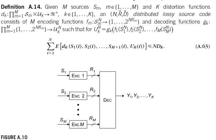
APPENDIX A: Formal Definitions and Notations . . . . 23

Notation. . . . 23

Centralized Source Coding . . . 25

Distributed Source Coding . . . 26

Remote Source Coding . . . 27

References . . . . 28

Distributed Source Coding: Theory, Algorithms, and Applications

4

CHAPTER 1

Foundations of Distributed Source Coding

1.1

INTRODUCTION

Data compression is one of the oldest and most important signal processing ques-tions. A famous historical example is the Morse code, created in 1838, which gives shorter codes to letters that appear more frequently in English (such as “e” and “t”). A powerful abstraction was introduced by Shannon in 1948 [1]. In his framework, the original source information is represented by a sequence of bits (or, equivalently, by one out of a countable set of prespecified messages). Classically, all the

informa-tion to be compressed was available in one place, leading to centralized encoding

problems. However, with the advent of multimedia, sensor, and ad-hoc networks, the

most important compression problems are now distributed: the source information

appears at several separate encoding terminals. Starting with the pioneering work of Slepian and Wolf in 1973, this chapter provides an overview of the main advances of the last three and a half decades as they pertain to the fundamental performance

bounds in distributed source coding. A first important distinction is losslessversus

lossy compression, and the chapter provides closed-form formulas wherever

possi-ble. A second important distinction isdirectversusremotecompression; in the direct

compression problem, the encoders have direct access to the information that is of interest to the decoder, while in the remote compression problem, the encoders only access that information indirectly through a noisy observation process (a famous exam-ple being the so-called CEO problem). An interesting insight discussed in this chapter concerns the sometimes dramatic (and perhaps somewhat unexpected) performance difference between direct and remote compression. The chapter concludes with a short discussion of the problem of communicating sources across noisy channels, and thus, Shannon’s separation theorem.

1.2

CENTRALIZED SOURCE CODING

1.2.1

Lossless Source Coding

The most basic scenario of source coding is that of describing source output sequences with bit strings in such a way that the original source sequence can be recovered without loss from the corresponding bit string. One can think about this scenario in two ways. First, one can map source realizations to binary strings of different lengths and strive to minimize the expected length of these codewords. Compres-sion is attained whenever some source output sequences are more likely than others: the likelier sequences will receive shorter bit strings. For centralized source coding

(see Figure 1.1), there is a rich theory of such codes (including Huffman codes,

S R DEC

ENC

ˆ

S

FIGURE 1.1

Centralized source coding.

goes to infinity. The main insight is that it is sufficient to assign bit strings to “typical” source output sequences. One measures the performance of a lossless source code by considering the ratioN/Lof the number of bits N of this bit string to the num-ber of source samples L. An achievable rate R⫽N/L is a ratio that allows for an asymptotically small reconstruction error.

Formal definitions of a lossless code and an achievable rate can be found in Appendix A (Definitions A.6 and A.7). The central result of lossless source coding

is the following:

Theorem 1.1. Given a discrete information source{S(n)}n⬎0, the rateRis achievable via

lossless source coding ifR⬎H_⬁(S), whereH_⬁(S) is the entropy (or entropy rate) of the source. Conversely, ifR⬍H_⬁(S),Ris not achievable via lossless source coding.

A proof of this theorem for the i.i.d. case and Markov sources is due to Shannon [1]. A proof of the general case can be found, for example, in [2,Theorem 3, p. 757].

1.2.2

Lossy Source Coding

In many source coding problems, the available bit rate is not sufficient to describe the information source in a lossless fashion. Moreover, for real-valued sources, loss-less reconstruction is not possible for any finite bit rate. For instance, consider a

source whose samples are i.i.d. and uniform on the interval[0,1]. Consider the binary

representation of each sample as the sequence.B1B2. . .; here, each binary digit is

independent and identically distributed (i.i.d.) with probability 1/2 of being 0 or 1.

Thus, the entropy of any sample is infinite, and Theorem1.1 implies that no finite rate

can lead to perfect reconstruction.

Instead, we want to use the available rate to describe the source to within the smallest possible averagedistortion D, which in turn is determined by a distortion functiond(·,·), a mapping from the source and reconstruction alphabets to the non-negative reals. The precise shape of the distortion functiond(·,·)is determined by the application at hand. A widely studied choice is the mean-squared error, that is, d(s,sˆ)⫽|s⫺ˆs|2.

6

CHAPTER 1

Foundations of Distributed Source Coding

be characterized compactly as a “single-letter”optimization problem usually called the rate-distortion function.More formally, we have the following theorem:

Theorem 1.2. Given a discrete memoryless source {S(n)}n⬎0 and bounded distortion

functiond:S⫻Sˆ→R⫹, a rateRis achievable with distortionDforR⬎RS(D), where

RS(D)⫽ min p(ˆs|s):

E[d(S,Sˆ)]⭐D

I(S; ˆS) (1.1)

is the rate distortion function. Conversely, forR⬍RS(D), the rateRis not achievable with distortionD.

A proof of this theorem can be found in [3, pp. 349–356]. Interestingly, it can also be shown that whenD⬎0,R⫽RS(D)is achievable [4].

Unlike the situation in the lossless case, determining the rate-distortion func-tion requires one to solve an optimizafunc-tion problem. The Blahut–Arimoto algorithm [5, 6] and other techniques (e.g., [7]) have been proposed to make this computation efficient.

While Theorem 1.2 is stated for discrete memoryless sources and a bounded distor-tion measure, it can be extended to continuous sources under appropriate technical conditions. Furthermore, one can show that these technical conditions are satisfied for memoryless Gaussian sources with a mean-squared error distortion. This is some-times called the quadratic Gaussian case. Thus, one can use Equation (1.1) in Theorem 1.2 to deduce the following.

Proposition 1.1. Given a memoryless Gaussian source {S(n)}n⬎0 with S(n)∼

N(0,␴2)and distortion function d(s,ˆs)⫽(s⫺ˆs)2,

RS(D)⫽ 1 2log

⫹␴2

D. (1.2)

For general continuous sources,the rate-distortion function can be difficult to deter-mine. In lieu of computing the rate-distortion function exactly, an alternative is to find closed-form upper and lower bounds to it. The idea originates with Shannon’s work [8], and it has been shown that under appropriate assumptions, Shannon’s lower bound for difference distortions (d(s,sˆ)⫽f(s⫺ˆs)) becomes tight in the high-rate regime [9].

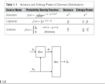
For a quadratic distortion and memoryless source{S(n)}n⬎0with variance␴_S2and entropy powerQS, these upper and lower bounds can be expressed as [10, p. 101]

1 2log

QS

D ⭐RS(D)⭐ 1 2log

␴2 S

D, (1.3)

Table 1.1 Variance and Entropy Power of Common Distributions

Source Name Probability Density Function Variance Entropy Power

Gaussian f(x)⫽√ 1

2␲e␴2e⫺( x⫺␮)2_/2␴2

␴2 _␴2

Laplacian f(x)⫽␭₂e⫺␭|x⫺␮| _␭22

e

␲·␭22

Uniform f(x)⫽

1

2a, ⫺a⭐x⫺␮⭐a

0, otherwise

a2

3 ␲6e·

a2

3

S₁

S₂ ENC

R

DEC Sˆ₁

FIGURE 1.2

Conditional rate distortion.

The conditional source coding problem (see Figure 1.2) considers the case in which a correlated source is available to the encoder and decoder to potentially decrease the encoding rate to achieve the same distortion. Definitions A.10 and A.11 formalize the problem.

Theorem 1.3. Given a memoryless source S1, memoryless source side information S2

available at the encoder and decoder with the property thatS1(k),S2(k)

are i.i.d. ink, and distortion functiond:S1⫻Sˆ1→⫹, the conditional rate-distortion function is

RS_1|S2(D)⫽ min p(sˆ1|s1,s2): E[d(S1,Sˆ1)]⭐D

I(S1; ˆS1|S2). (1.4)

A proof of Theorem 1.3 can be found in [11,Theorem 6, p. 11].

8

CHAPTER 1

Foundations of Distributed Source Coding

1.2.3

Lossy Source Coding for Sources with Memory

We start with an example. Consider a Gaussian sourceS with S(i)∼N(0,2)where

pairsY(k)⫽(S(2k⫺1),S(2k))have the covariance matrix

⌺⫽

2 1

1 2

, (1.5)

andY(k)are i.i.d. overk. The discrete Fourier transform (DFT) of each pair can be

written as

˜

S(2k⫺1)⫽√1

2(S(2k⫺1)⫹S(2k)) (1.6)

˜

S(2k)⫽√1

2(S(2k⫺1)⫺S(2k)), (1.7)

which has the covariance matrix

˜ ⌺⫽ 3 0 0 1

, (1.8)

and thus the sourceS˜is independent,with i.i.d. even and odd entries. For squared error

distortion, ifC is the codeword sent to the decoder, we can express the distortion as

nD⫽n_i⫽1E[(S(i)⫺E[S(i)|C])2]. By linearity of expectation, it is possible to rewrite this as

nD⫽

n

i⫽1

E S˜(i)⫺E[˜S(i)|C]2

(1.9)

⫽ n/2

k⫽1

E S˜(2k⫺1)⫺E[˜S(2k⫺1)|C]2

⫹ n/2

k⫽1

E S˜(2k)⫺E[˜S(2k)|C]2

.

(1.10) Thus, this is a rate-distortion problem in which two independent Gaussian sources of different variances have a constraint on the sum of their mean-squared errors. Sometimes known as the parallel Gaussian source problem, it turns out there is a well-known solution to it called reverse water-filling [3, p. 348,Theorem 13.3.3], which in this case, evaluates to the following:

RS(D)⫽

1 2log ␴2 1 D1 ⫹1 2log ␴2 2 D2

(1.11)

Di⫽

␯, ␯⬍␴2 i, ␴2

i, ␯⭓␴i2,

(1.12)

where␴₁2⫽3,␴₂2⫽1, and␯is chosen so thatD1⫹D2⫽D.

Proposition 1.2. Let S be a stationary ergodic Gaussian source with autocorrela-tion funcautocorrela-tion E[SnSn⫺k]⫽␾(k)and power spectral density

⌽(␻)⫽ ⬁ k⫽⫺⬁

␾(k)e⫺jk␻. (1.13)

Then the rate-distortion function for S under mean-squared error distortion is given by:

R(D_␯)⫽ 1 4␲

_␲

⫺␲max

0,log⌽(␻) ␯

d␻ (1.14)

D_␯⫽ 1 2␲

_␲

⫺␲min{␯,⌽(␻)}d␻. (1.15)

PROOF. See Berger [10, p. 112]. ■

While it can be difficult to evaluate this in general,upper and lower bounds can give a better sense for its behavior. For instance,let␴2be the variance of a stationary ergodic Gaussian source. Then a result of Wyner and Ziv [14] shows that the rate-distortion function can be bounded as follows:

1 2log

␴2

D ⫺⌬S⭐RS(D)⭐ 1 2log

␴2

D, (1.16)

where⌬S is a constant that depends only on the power spectral density ofS.

1.2.4

Some Notes on Practical Considerations

The problem formulation considered in this chapter focuses on the existence of codes for cases in which the encoder has access to the entire source noncausally and knows its distribution. However,in many situations of practical interest,some of these assump-tions may not hold. For instance,several problems have considered the effects of delay and causal access to a source [15–17]. Some work has also considered cases in which no underlying probabilistic assumptions are made about the source [18–20]. Finally, the work of Gersho and Gray [21] explores how one might actually go about designing implementable vector quantizers.

1.3

DISTRIBUTED SOURCE CODING

The problem of source coding becomes significantly more interesting and challenging in a network context. Several new scenarios arise:

■ Different parts of the source information may be available to separate encoding terminals that cannot cooperate.

10

CHAPTER 1

Foundations of Distributed Source Coding

We start our discussion by an example illustrating the classical problem of source coding with side information at the decoder.

Example 1.1

Let{S(n)}n_⬎0be a source where source samplesS(n) are uniform over an alphabet of size 8,

which we choose to think of as binary vectors of length 3. The decoder has access to a corrupted version of the source{˜S(n)}n_⬎0where each sampleS˜(n) takes values in a set of

ternary sequences{0,∗,1}3of length 3 with the property that

Pr

˜

S(n)⫽(c1,c2,c3)S(n)⫽(b1,b2,b3)⫽

⎧ ⎪ ⎪ ⎪ ⎪ ⎪ ⎨ ⎪ ⎪ ⎪ ⎪ ⎪ ⎩

1

4, if(c1,c2,c3)⫽(b1,b2,b3) 1

4, if(c1,c2,c3)⫽(∗,b2,b3) 1

4, if(c1,c2,c3)⫽(b1,∗,b3) 1

4, if(c1,c2,c3)⫽(b1,b2,∗)

(1.17)

Thus, the decoder has access to at least two of every three bits per source symbol, but the encoder is unaware of which ones. Consider the partition of the alphabetS into

S1⫽

(0,0,0), S2⫽

(1,1,1),

(0,1,1), (1,0,0),

(1,1,0), (0,0,1),

(1,0,1)

(0,1,0)

. (1.18)

If the decoder knows which of these partitions a particular sampleS(n) is in,S˜(n) is sufficient to determine the exact value ofS(n). Thus, for each source output, the encoder can use one bit to indicate to which of the two partitions the source sample belongs. Thus, at a rate of 1 bit per source sample, the decoder can perfectly reconstruct the output. However, in the absence of{˜S(n)}n⬎0at the decoder, Theorem 1.1 implies the best possible rate isH(S1)⫽3

bits per source sample.

Example 1.1 illustrates a simple version of a strategy known asbinning. It turns out that binning can be applied more generally and is used to prove many of the results in distributed source coding.

1.3.1

Lossless Source Coding

More generally,we now consider the scenario illustrated in Figure1.3,where two

ˆ ˆ

S₂ R₂

S₁

S₁,S₂ R₁

ENC

ENC

DEC

FIGURE 1.3

Distributed source coding problem.

assumeR2⬎log|S2|, we can assume that the decoder knowsS2 without error, and thus this problem also includes the special case of side information at the decoder. Theorem 1.4. Given discrete memoryless sourcesS1andS2, defineRas

R⫽

(R1,R2):R1⫹R2⭓H(S1,S2),

R1⭓H(S1|S2),R2⭓H(S2|S1)

. (1.19)

Furthermore, letR0 _{be the interior ofR. Then (R}

1,R2)∈R0 are achievable for the

two-terminal lossless source coding problem, and (R1,R2) /∈Rare not.

The proof of this result was shown by Slepian and Wolf [22]; to show achievability involves a random binning argument reminiscent of Example 1.1. However,by contrast to that example, the encoders now bin over the entire vector of source symbols, and they only get probabilistic guarantees that successful decoding is possible.

Variations and extensions of the lossless coding problem have been considered by Ahlswede and Körner [23], who examine a similar setup case in which the decoder is only interested inS1;Wyner [24], who considers a setup in which one again wants to reconstruct sourcesS1andS2, but there is now an additional encoding terminal with access to another correlated information sourceS3;and Gel’fand and Pinsker [25],who consider perfect reconstruction of a source to which each encoding terminal has only a corrupted version. In all of these cases, a random binning strategy can be used to establish optimality. However, one notable exception to this is a paper by Körner and Marton [26], which shows that when one wants to reconstruct the modulo-2 sum of correlated sources, there exists a strategy that performs better than binning.

1.3.2

Lossy Source Coding

By analogy to the centralized compression problem, it is again natural to study the problem where instead of perfect recovery, the decoder is only required to provide estimates of the original source sequences to within some distortions. Reconsidering

Figure1.3,we now ask that the sourceS1be recovered at distortionD1,when assessed

12

CHAPTER 1

Foundations of Distributed Source Coding

measured2(·,·).The question is again to determine the necessary rates,R1 andR2, respectively, as well as the coding schemes that permit satisfying the distortion con-straints. Formal definitions are provided in Appendix A (Definitions A.14 and A.15). For this problem,a natural achievable strategy arises. One can first quantize the sources at each encoder as in the centralized lossy coding case and then bin the quantized val-ues as in the distributed lossless case. The work of Berger and Tung [27–29] provides an elegant way to combine these two techniques that leads to the following result. The result was independently discovered by Housewright [30].

Theorem 1.5:“Quantize-and-bin.” Given sourcesS1andS2with distortion functionsdk:

Sk⫻Uk→⫹,k∈{1,2}, the achievable rate-distortion region includes the following set:

R⫽{(R,D):∃U1,U2s.t.U1⫺S1⫺S2⫺U2,

E[d1(S1,U1)]⭐D1,E[d2(S2,U2)]⭐D2, (1.20)

R₁⬎I(S₁;U₁|U₂),R₂⬎I(S₂;U₂|U₁), R₁⫹R₂⬎I(S₁,S₂;U₁U₂)}.

A proof for the setting of more than two users is given by Han and Kobayashi [31, Theorem 1, pp. 280–284]. A major open question stems from the optimality of the “quantize-and-bin” achievable strategy. While work by Servetto [32] suggests it may be tight for the two-user setting, the only case for which it is known is the quadratic Gaussian setting, which is based on an outer bound developed by Wagner and Anantharam [33, 34].

Theorem 1.6: Wagner, Tavildar, and Viswanath [35]. Given sourcesS1 andS2 that are

jointly Gaussian and i.i.d. in time, that is,S1(k),S2(k)

∼N(0,⌺), with covariance matrix ⌺⫽

␴2

1 ␳␴1␴2

␳␴1␴2 ␴22

(1.21)

forD1,D2⬎0 defineR(D1,D2) as

R(D1,D2)⫽

(R1,R2):R1⭓ 1 2log

⫹(1⫺␳2⫹␳22⫺2R2)␴21

D1

,

R2⭓ 1 2log

⫹(1⫺␳2⫹␳22⫺2R1)␴22

D2

,

R1⫹R2⭓ 1 2log

⫹(1⫺␳2)␴21␴22␤(D1,D2) 2D1D2

, (1.22)

where

␤(D1,D2)⫽1⫹

1⫹ 4␳ 2_D

1D2 (1⫺␳2₎2_␴2

1␴22

. (1.23)

Furthermore, letR0 be the interior ofR. Then for distortionsD1,D2⬎0,(R1,R2)∈

R0_(D

ˆ

S₂ S₁

S₁ R₁

ENC

DEC

FIGURE 1.4

The Wyner–Ziv source coding problem.

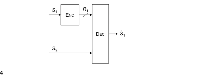
In some settings,the rates given by the“quantize-and-bin”achievable strategy can be shown to be optimal. For instance, consider the setting in which the second encoder has an unconstrained rate link to the decoder, as in Figure 1.4. This configuration is often referred to as the Wyner–Ziv source coding problem.

Theorem 1.7. Given a discrete memoryless sourceS1, discrete memoryless side

informa-tion sourceS2with the property that (S1(k),S2(k)) are i.i.d. overk, and bounded distortion

functiond:S⫻U→⫹, a rateRis achievable with lossy source coding with side information at the decoder and with distortionDifR⬎RWZ_S

1|S2(D). Here RWZ_S

1|S2(D)⫽ _pmin_(u|s): U⫺S1⫺S2 E[d(S1,U)]⭐D

I(S1;U|S2) (1.24)

is the rate distortion function for side information at the decoder. Conversely, for R⬍RWZ_S

1|S2(D), the rateRis not achievable with distortionD.

Theorem 1.7 was first proved by Wyner and Ziv [36]. An accessible summary of the proof is given in [3,Theorem 14.9.1, pp. 438–443].

The result can be extended to continuous sources and unbounded distortion mea-sures under appropriate regularity conditions [37]. It turns out that for the quadratic Gaussian case, that is, jointly Gaussian source and side information with a mean-squared error distortion function, these regularity conditions hold, and one can char-acterize the achievable rates as follows. Note the correspondence between this result and Theorem 1.6 asR2→⬁.

Proposition 1.3. Consider a source S1 and side information source S2 such that

(S1(k),S2(k))∼N(0,⌺)are i.i.d. in k, with

⌺⫽␴2

1 ␳

␳ 1

(1.25)

Then for distortion function d(s1,u)⫽(s1⫺u)2and for D⬎0, RWZ_S

1|S2(D)⫽ 1 2log

⫹(1⫺␳2)␴2

14

CHAPTER 1

Foundations of Distributed Source Coding

1.3.2.1

Rate Loss

Interestingly, in this Gaussian case, even if the encoder in Figure1.4alsohad access to

the sourceX2as in the conditional rate-distortion problem,the rate-distortion function would still be given by Proposition 1.3. Generally, however, there is a penalty for the absence of the side information at the encoder. A result of Zamir [38] has shown that for memoryless sources with finite variance and a mean-squared error distortion, the rate-distortion function provided in Theorem 1.7 can be no larger than 1₂ bit/source sample than the rate-distortion function given in Theorem 1.3.

It turns out that this principle holds more generally. For centralized source coding of a length M zero-mean vector Gaussian source {S(n)}n⬎0 with covariance matrix ⌺S having diagonal entries␴2S and eigenvalues␭(

M) 1 , . . . ,␭(

M)

M with the property that ␭(M)

m ⭓␧ for some␧⬎0 and allm, and squared error distortion, the rate-distortion function is given by [10]

R_S(D)⫽ M

m⫽1 1 2log

␭m

Dm, (

1.27)

Dm⫽

␯ ␯⬍␭m,

␭m otherwise, (

1.28)

whereM_m⫽1Dm⫽D. Furthermore, it can be lower bouned by [39] R_S(D)⭓M

2 log M␧

D . (1.29)

Suppose each component{Sm(n)}n⬎0were at a separate encoding terminal. Then it is possible to show that by simply quantizing, without binning, an upper bound on the sum rate for a distortionDis given by [39]

M

m⫽1 Rm⭐

M 2 log

1⫹M␴

2 S D

. (1.30)

Thus, the scaling behavior of (1.27) and (1.30) is the same with respect to both small Dand largeM.

1.3.2.2

Optimality of “Quantize-and-bin” Strategies

In addition to Theorems1.6 and 1.7,“quantize-and-bin” strategies have been shown to

be optimal for several special cases, some of which are included in the results of Kaspi and Berger [40]; Berger and Yeung [41]; Gastpar [42]; and Oohama [43].

1.3.2.3

Multiple Descriptions Problem

Most of the problems discussed so far have assumed a centralized decoder with access to encoded observations from all the encoders. A more general model could also include multiple decoders, each with access to only some subset of the encoded observations.While little is known about the general case,considerable effort has been devoted to studying the multiple descriptions problem. This refers to the specific case of a centralized encoder that can encode the source more than once, with subsets of these different encodings available at different encoders. As in the case of the distributed lossy source coding problem above, results for several special cases have been established [45–55].

1.3.3

Interaction

Consider Figure1.5, which illustrates a setting in which the decoder has the ability to

communicate with the encoder and is interested in reconstructingS. Seminal work by Orlitsky [56, 57] suggests that under an appropriate assumption, the benefits of this kind of interaction can be quite significant. The setup assumes two random variables Sand U with a joint distribution, one available at the encoder and the other at the decoder. The decoder wants to determineS with zero probability of error, and the goal is to minimize the total number of bits used over all realizations ofSandUwith positive probability. The following example illustrates the potential gain.

Example 1.2

(The League Problem [56]) Let S be uniformly distributed among one of 2m teams in a softball league.Scorresponds to the winner of a particular game and is known to the encoder. The decoder knowsU, which corresponds to the two teams that played in the tournament. Since the encoder does not know the other competitor in the game, if the decoder cannot communicate with the encoder, the encoder must sendmbits in order for the decoder to determine the winner with zero probability of error.

Now suppose the decoder has the ability to communicate with the encoder. It can simply look for the first position at which their binary expansion differs and request that from the encoder. This request costs log₂mbits since the decoder simply needs to send one of them

different positions. Finally, the encoder simply sends the value ofSat this position, which costs an additional 1 bit. The upshot is that asmgets larger, the noninteractive strategy requires

exponentially more bitsthan the interactive one.

S

ENC DEC

ˆ S

U

FIGURE 1.5

16

CHAPTER 1

Foundations of Distributed Source Coding

1.4

REMOTE SOURCE CODING

In many of the most interesting source coding scenarios, the encoders do not get to observe directly the information that is of interest to the decoder. Rather, they may observe a noisy function thereof. This occurs, for example, in camera and sensor

networks. We will refer to such source coding problems asremote source coding.In

this section, we discuss two main insights related to remote source coding:

1. For the centralized setting, direct and remote source coding are the same thing, except with respect to different distortion measures (see Theorem 1.8). 2. For the distributed setting, how severe is the penalty of distributed coding

versus centralized? For direct source coding, one can show that the penalty is often small. However, for remote source coding, the penalty can be dramatic (see Equation(1.47)).

The remote source coding problem was initially studied by Dobrushin and Tsybakov [58]. Wolf and Ziv explored a version of the problem with a quadratic dis-tortion, in which the source is corrupted by additive noise, and found an elegant decoupling between estimating the noisy source and compressing the estimate [59]. The problem was also studied by Witsenhausen [60].

We first consider the centralized version of the problem before moving on to the distributed setting. For simplicity, we will focus on the case in which the source and observation processes are memoryless.

1.4.1

Centralized

The remote source coding problem is depicted in Figure1.6, and Definitions A.16 and

A.17 provide a formal description of the problem.

Consider the case in which the source and observation process are jointly mem-oryless. In this setting, the remote source coding is equivalent to a standard source coding problem with a modified distortion function [10]. For instance, given a dis-tortion function d:S⫻Sˆ→⫹, one can construct the distortion function d˜:U⫻S, defined for allu∈U andsˆ∈ ˆSas

d(u,sˆ)⫽E[d(S,sˆ)|U⫽u], (1.31)

where (S,U)share the same distribution as (S1,U1). The following result is then straightforward from Theorem 1.2.

ˆ

S U R S

ENC OBS

SRC DEC SNK

FIGURE 1.6

In the remote source coding problem, one no longer has direct access to the underlying sourceS

Theorem 1.8:Remote rate-distortion theorem [10]. Given a discrete memoryless source S, bounded distortion function d:S⫻Sˆ→⫹, and observations Usuch that S(k),U(k) are i.i.d. ink, the remote rate-distortion function is

Rremote_S (D)⫽ min p(ˆs|u):ˆS⫺U⫺S

E[d(S,Sˆ)]⭐D

I(U; ˆS). (1.32)

This theorem extends to continuous sources under suitable regularity conditions, which are satisfied by finite-variance sources under a squared error distortion. Theorem 1.9:Additive remote rate-distortion bounds. For a memoryless sourceS, bounded distortion functiond:S⫻Sˆ→⫹, and observationsUi⫽Si⫹Wi,whereWi is a sequence of i.i.d. random variables,

1 2log

QV D⫺D0⭐

Rremote_S (D)⭐1 2log

␴2

V

D⫺D0, (

1.33)

whereV⫽E[S|U], andD0⫽E(S⫺V)2, and where

QSQW QU ⭐D0⭐

␴2

S␴W2 ␴2

U

. (1.34)

This theorem does not seem to appear in the literature, but it follows in a relatively straightforward fashion by combining the results of Wolf and Ziv [59] with Shannon’s upper and lower bounds. In addition, for the case of a Gaussian sourceSand Gaussian observation noise W, the bounds in both (1.33) and (1.34) are tight. This can be verified using Table 1.1.

Let us next consider the remote rate-distortion problem in which the encoder makesM⭓1 observations of each source sample. The goal is to illustrate the depen-dence of the remote rate-distortion function on the number of observations M. To keep things simple, we restrict attention to the scenario shown in Figure 1.7.

ENC DEC

S Sˆ

W₁

U₁

W₂

U₂

WM

UM

R

FIGURE 1.7

18

CHAPTER 1

Foundations of Distributed Source Coding

More precisely, we suppose thatS is a memoryless source and that the observation process is

Um(k)⫽S(k)⫹Wm(k), k⭓1, (1.35) whereWm(k)are i.i.d. (both inkand inm) Gaussian random variables of mean zero and variance␴_W2

m.For this special case, it can be shown [61, Lemma 2] that for any given timek,we can collapse allM observations into a single equivalent observation, characterized by

U(k)⫽ 1 M

M

m⫽1 ␴2

W ␴2

Wm

Um(k) (1.36)

⫽S(k)⫹ 1 M

M

m⫽1 ␴2

W ␴2

Wm

Wm(k), (1.37)

where␴_W2 ⫽

1 M

M

m⫽1_␴21 Wm

_⫺1

.This works becauseU(k)is a sufficient statistic for S(k) given U1(k), . . . ,UM(k). However, at this point, we can use Theorem 1.9 to obtain upper and lower bounds on the remote rate-distortion function. For exam-ple, using(1.34), we can observe that as long as the sourceSsatisfiesh(S)⬎⫺⬁,D0 scales linearly with␴_W2 ,and thus, inversely proportional toM.

When the source is Gaussian, a precise characterization exists. In particular, Equa-tions(1.33)and(1.34)allow one to conclude that the rate-distortion function is given by the following result.

Proposition 1.4. Given a memoryless Gaussian source S with S(i)∼N(0,␴_S2), squared error distortion, and the M observations corrupted by an additive Gaussian noise model and given by Equation (1.35), the remote rate-distortion function is

Rremote_S (D)⫽1 2log ␴2 S D ⫹ 1 2log ␴2 S ␴2 U⫺ ␴2

W␴S2 MD

, (1.38)

where

␴2 U⫽␴S2⫹

␴2 W

M and ␴

2 W⫽ 1 1 M M

m⫽1 1

␴2 Wm

. (1.39)

As in the case of direct source coding, there is an analogous result for the case of jointly stationary ergodic Gaussian sources and observations.

⌽S,U(␻)be their corresponding power and cross spectral densities.Then for mean-squared error distortion, the remote rate-distortion function is given by

Rremote_S (D_␯)⫽ 1 4␲

_␲

⫺␲max

0,|⌽S,U(␻)| 2 ␯⌽U(␻)

d␻ (1.40)

D_␯⫽ 1 2␲

_␲

⫺␲

_⌽

S(␻)⌽U(␻)⫺|⌽S,U(␻)|2 ⌽U(␻)

d␻

⫹ 1 2␲

_␲

⫺␲min

␯,|⌽S,U(␻)|2 ⌽U(␻)

d␻. (1.41)

PROOF. See Berger [10, pp. 124–129]. ■

Observe that ₂1_␲⫺␲␲

_⌽

S(␻)⌽U(␻)⫺|⌽S,U(␻)|2 ⌽U(␻)

d␻is simply the mean-squared error resulting from applying a Wiener filter onU to estimateS.

1.4.2

Distributed: The CEO Problem

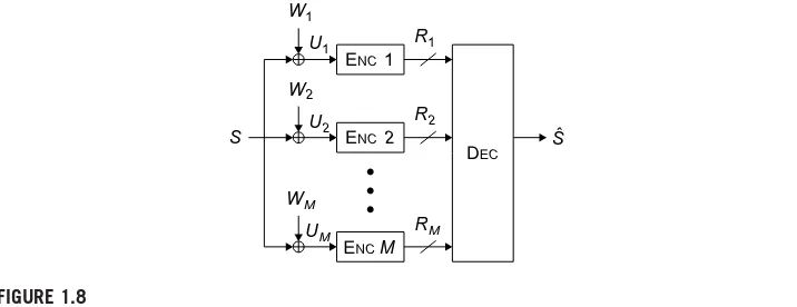
Let us now turn to the distributedversion of the remote source coding problem.

A particularly appealing special case is illustrated in Figure1.8. This problem is often

motivated with the following scenario. A chief executive officer or chief estimation officer (CEO) is interested in estimating a random process.M agents observe noisy versions of the random process and have noiseless bit pipes with finite rate to the CEO. Under the assumption that the agents cannot communicate with one another, one wants to analyze the fidelity of the CEO’s estimate of the random process sub-ject to these rate constraints. Because of the scenario, this is often called the CEO problem [62].

A formal definition of the CEO problem can be given by a slight variation of Definition A.15, namely, by adding an additional encoder with direct access to the underlying source, and considers the rate-distortion region when the rate of this

ENC 1

ENC 2

ENC M

DEC

S _Sˆ

W₁

U₁ R1

W2

U₂ R2

WM

UM RM

FIGURE 1.8

20

CHAPTER 1

Foundations of Distributed Source Coding

encoder is set to zero. The formal relationship is established in Definitions A.18 and A.19.

The CEO problem has been used as a model for sensor networks, where the encoders correspond to the sensors, each with access to a noisy observation of some state of nature. Unfortunately (and perhaps not too surprisingly), the general CEO problem remains open. On the positive side, the so-calledquadratic GaussianCEO problem has been completely solved. Here, with respect to Figure 1.8, the source S is a memoryless Gaussian source, and the noisesWm(k)are i.i.d. (both in k and in m) Gaussian random variables of mean zero and variance␴_W2

m.The setting was first considered by Viswanathan and Berger [63], and later refined (see, e.g. [43, 64, 65] or [66, 67]), leading to the following theorem:

Theorem 1.10. Given a memoryless Gaussian sourceSwithS(i)∼N(0,␴2

S), squared error distortion, and theMobservations corrupted by an additive Gaussian noise model and given by Equation (1.35), and assume that␴2

W1⭐␴

2

W2⭐· · ·⭐␴

2

WM. Then the sum rate-distortion function for the CEO problem is given by

RCEO_S (D)⫽1 2log ␴2 S D ⫺ 1 2log _K

m⫽1

␴2 Wm ⫺K 2log 1 KDK ⫺ 1 KD

, (1.42)

whereKis the largest integer in{1,. . .,M}satisfying 1

D⫺ 1 ␴2

S

⭓⫺K⫺1 ␴2

WK ⫹

K⫺1

m⫽1 1 ␴2

Wm

(1.43)

and 1 DK⫽ 1 ␴2 S ⫹ K

m⫽1 1 ␴2

Wm

. (1.44)

Furthermore, if␴_W2

m⫽␴

2

W for allm⫽1, . . . ,M,

RCEO_S (D)⫽1 2log ␴2 S D ⫹ M 2 log ␴2 S ␴2 U⫺ ␴2

W␴2S MD

, (1.45)

where

␴2 U⫽␴S2⫹

␴2 W

M . (1.46)

Alternate strategies for achieving the sum rate have been explored [68] and achievable strategies for the case of vector-Gaussian sources have been studied [69, 70], but the rate region for this setting remains open.

equal noise variances␴2_W

m⫽␴

2

W, this rate loss is exactly characterized by comparing Proposition 1.4 with Theorem 1.10, leading to

RCEO_S (D)⫺Rremote_S (D)⫽M⫺1

2 log ␴2 S ␴2 S⫹ ␴2 W M (1⫺

␴2 S D)

. (1.47)

By lettingM→⬁, this becomes

RCEO_S (D)⫺Rremote_S (D)⫽␴ 2 W 2 1 D⫺ 1 ␴2 S

, (1.48)

so the rate loss scales inversely with the target distortion. Note that this behavior is dramatically different from the one found in Section 1.3.2.1; as we have seen there, for directsource coding, both centralized and distributed encoding have the same scaling law behavior with respect to largeM and small D (at least under the assumptions stated in Section 1.3.2.1). By contrast, as the quadratic Gaussian example reveals, for remotesource coding, centralized and distributed encoding can have very different scaling behaviors.

It turns out that the quadratic Gaussian example has the worst case rate loss behavior among all problems that involve additive Gaussian observation noise and mean-squared error distortion (but arbitrary statistics of the sourceS). More precisely, we have the following proposition, proved in [61]:

Proposition 1.6. Given a real-valued zero-mean memoryless source S with variance ␴2

S, squared error distortion, and the M observations corrupted by an additive Gaussian noise model and given by Equation (1.35) with␴_W2

i⫽␴

2

W, the difference between the sum distortion function for the CEO problem and the remote rate-distortion function is no more than

RCEO_S (D)⫺Rremote_S (D)⭐M⫺1

2 log ␴2 S ␴2 S⫹ ␴2 W M (1⫺

␴2 S D)

⫹1 2log

(M⫺1)D␴2

W⫹␴2S(M(2D⫹2 √

D␴2

W)⫺MD(D⫹2 √

D␴2 W))

D(M␴_S2⫹␴_W2)⫺␴_W2␴2_S . (1.49) By letting M→⬁, this becomes

RCEO_S (D)⫺Rremote_S (D)⭐␴ 2 W 2 1 D⫺ 1 ␴2 S ⫹1 2log 1⫹ 1 D⫺ 1 ␴2 S

(D⫹2

D␴_W2)

. (1.50) Thus, the rate loss cannot scale more than inversely with the distortion Deven for non-Gaussian sources. Bounds for the rate loss have been used to give tighter achievable bounds for the sum rate when the source is non-Gaussian [71].

22

CHAPTER 1

Foundations of Distributed Source Coding

1.5

JOINT SOURCE-CHANNEL CODING

When information is to be stored on a perfect (error-free) discrete (e.g., binary) medium, then the source coding problem surveyed in this chapter is automatically relevant. However, in many tasks, the source information is compressed because it must be communicated across a noisy channel. There, it is not evident that the formal-izations discussed in this chapter are relevant. For the stationary ergodic point-to-point

problem,Shannon’sseparation theoremproves that,indeed,an optimal architecture is

to first compress the source information down to the capacity of the channel,and then communicate the resulting encoded bit stream across the noisy channel in a reliable fashion.

To make this precise, we discuss the scenario illustrated in Figure1.9. Formally,

consider the following class of noisy channels:

Definition 1.1. Given a random vectorXn, a discrete memoryless channel (used without feedback) is characterized by a conditional distributionp(y|x) such that for a given channel inputxn,the channel outputYnsatisfies

Pr(Yn⫽yn|Xn⫽xn)⫽ n

i⫽1

Pr(Y(i)⫽y(i)|X(i)⫽x(i)), (1.51)

wherePr(Y(i)⫽y|X(i)⫽x)⫽p(y|x).

Moreover, by reliable communication, we mean the following:

Definition 1.2. Given a sourceSand discrete memoryless channelp(y|x), an (N,␣,␦) loss-less joint source-channel codeconsists of an encoding functionf:SN_→XK_{and decoding} functiong:YK_→SN_{such thatX}K_⫽f(SN_{) and}

Pr(SK⫽g(YK))⭐␦, (1.52)

where␣K⫽N. Thus,␣is sometimes called themismatchof the source to the channel. Definition 1.3. A sourceSisrecoverableover a discrete memoryless channelp(y|x) with mismatch␣if for all␦⬎0, there existsN∗such that for allN⭓N∗, there exists an (N,␣,␦) lossless joint source-channel code.

Then, the so-called separation theorem can be expressed as follows:

Theorem 1.11: Joint Source-Channel Coding Theorem. A discrete memoryless source S is recoverable over a discrete memoryless channel p(y|x) with mismatch␣if H(S)⬍ ␣maxp(x)I(X;Y). Conversely, ifH(S)⬎␣maxp(x)I(X;Y), it is not recoverable.

ENC P (Y |X)

SRC S DEC SNK

N _XK _YK _SˆN

FIGURE 1.9

A proof of this theorem can be found, for example, in [3]. One should note that The-orem 1.11 can be stated more generally for both a larger class of sources and for channels.

The crux, however, is that there is no equivalent of the separation theorem in communicationnetworks.One of the earliest examples of this fact was given by [73]: when correlated sources are transmitted in a lossless fashion across a multiple-access channel, it isnotgenerally optimal to first compress the sources with the Slepian– Wolf code discussed in Section 1.3,thus obtaining smaller and essentially independent source descriptions,and sending these descriptions across the multiple-access channel using a capacity-approaching code. Rather, the source correlation can be exploited to access dependent input distributions on the multiple-access channels, thusenlarging the region of attainable performance. A more dramatic example was found in [74– 76]. In that example, modeling a simple “sensor”network, a single underlying source is observed byMterminals subject to independent noises.These terminals communicate over an additive multiple-access channel to a “fusion center” whose only goal is to recover the single underlying source to within the smallest squared error. For this problem, one may use the CEO source code discussed in Section 1.4.2, followed by a regular capacity-approaching code for the multiple-access channel. Then, the smallest squared error distortionD decreases like 1/logM. However, it can be shown that the optimal performance for a joint source-channel code decreases like 1/M, that is,exponentiallybetter. For some simple instances of the problem, the optimal joint source-channel code is simply uncoded transmission of the noisy observations [77]. Nevertheless, for certain classes of networks, one can show that a distributed source code followed by a regular channel code is good enough, thus establishing partial and approximate versions of network separation theorems. An account of this can be found in [78].

ACKNOWLEDGMENTS

The authors would like to acknowledge anonymous reviewers and others who went through earlier versions of this manuscript. In particular, Mohammad Ali Maddah-Ali

pointed out and corrected an error in the statement of Theorem1.10.

APPENDIX A: Formal Definitions and Notations

results in this chapter.

A.1

NOTATION

Unless otherwise stated, capital lettersX,Y,Z denote random variables, lower-case

24

CHAPTER 1

Foundations of Distributed Source Coding

The shorthandp(x,y),p(x), andp(y)will be used for the probability distributions Pr(X⫽x,Y⫽y),Pr(X⫽x), andPr(Y⫽y).XN will be used to denote the random vectorX1,X2, . . . ,XN.The alternate vector notationRandDwill sometimes be used to represent achievable rate-distortion regions. Finally,we will use the notationX⫺Y⫺Z to denote that the random variablesX,Y,Zform a Markov chain. That is,XandZare independent givenY.

We start by defining the notion of entropy, which will be useful in the sequel. Definition A.1. LetX,Ybe discrete random variables with joint distributionp(x,y). Then theentropy H(X) ofXis a real number given by the expression

H(X)⫽⫺E[logp(X)]⫽⫺ x

p(x)logp(x), (A.53)

thejoint entropy H(X,Y) ofX andY is a real number given by the expression H(X,Y)⫽⫺E[logp(X,Y)]⫽⫺

x,y

p(x,y)logp(x,y), (A.54)

and theconditional entropy H(X|Y) ofX givenY is a real number given by the expression H(X|Y)⫽⫺E[logp(X|Y)]⫽H(X,Y)⫺H(Y). (A.55) With a definition for entropy, we can now define mutual information.

Definition A.2. Let X,Y be discrete random variables with joint distribution p(x,y). Then the mutual information I(X;Y) between X and Y is a real number given by the expression

I(X;Y)⫽H(X)⫺H(X|Y)⫽H(Y)⫺H(Y|X). (A.56) Similar definitions exist in the continuous setting.

Definition A.3. LetX,Ybe continuous random variables with joint densityf(x,y). Then we define thedifferential entropy h(X)⫽⫺E[logf(X)],joint differential entropy h(X,Y)⫽ ⫺E[logf(X,Y)],conditional differential entropy h(X|Y)⫽⫺E[logf(X|Y)], andmutual infor-mation I(X;Y)⫽h(X)⫺h(X|Y)⫽h(Y)⫺h(Y|X).

Definition A.4. LetX be a continuous random variable with densityf(x). Then itsentropy power QXis given by

QX⫽ 1