Antenna Gain Enhancement and Beamshaping using a Diffractive Optical Element (DOE) Lens

Rochester Institute of Technology

RIT Scholar Works

Theses Thesis/Dissertation Collections

2014

Antenna Gain Enhancement and Beamshaping

using a Diffractive Optical Element (DOE) Lens

Christopher Torbitt

Follow this and additional works at:http://scholarworks.rit.edu/theses

This Thesis is brought to you for free and open access by the Thesis/Dissertation Collections at RIT Scholar Works. It has been accepted for inclusion in Theses by an authorized administrator of RIT Scholar Works. For more information, please [email protected].

Recommended Citation

i | P a g e

Antenna Gain Enhancement and Beamshaping using a

Diffractive Optical Element (DOE) Lens

By

Christopher Torbitt

A Thesis Submitted in Partial Fulfillment of the

Requirements of the Degree of

MASTER OF SCIENCE

In

Electrical Engineering

Approved by:

Professor: ____________________________________

(Dr. Jayanti Venkataraman – Advisor)

Professor: ____________________________________

(Dr. Zhaolin Lu - Committee Member)

Professor: ____________________________________

(Dr. Gill Tsouri - Committee Member)

Professor: ____________________________________

(Dr. Sohail A. Dianat – Department Head)

Department of Electrical and Microelectronic Engineering

Kate Gleason College of Engineering (KGCOE)

Rochester Institute of Technology

Rochester, New York

ii | P a g e

Acknowledgements

I would like to thank Dr. Venkataraman for her advice and guidance over the past

three years. Thank you for always pushing me to do my best through this process.

Most importantly I would like to thank my parents for always being there for me

and providing me with the opportunity to be where I am today. None of this would be

iii | P a g e

Abstract

Dielectric and metamaterial lenses have been designed for gain enhancement and

beam shaping. The motivation for this work came from a commercially available slotted

waveguide antenna with a dielectric lens that shapes the beam and enhances the gain only

in the azimuth plane. When two of these antennas, each with a dielectric lens, are

stacked as an array to form the sum and difference patterns the elevation plane gain is

low and the beam width too wide to be acceptable for radar applications.

The objective of the present work is to design a diffractive optical element (DOE)

lens for gain enhancement gain and beam shaping. As compared to other available lenses

it is much thinner, lighter and easily machined. The DOE lens is made from rexolite

which has a dielectric constant of 2.53. The DOE lens is composed of a series of zones

which focus the light at a certain focal length. The phase is the same everywhere on each

zone at the focal point. The phase difference between neighboring zones is 2π, resulting

in a constructive interference at the focus. These zones are able to focus the radiation

from an antenna in order to enhance the gain and shape the beam. The design parameters

include the lens diameter, number of zones, the center zone thickness for a particular

frequency and refractive index of the dielectric material.

A comprehensive study has been performed in CST Microwave Studio to

illustrate the properties of the DOE lens. The focusing property for image formation is

iv | P a g e

frequencies and with varying design parameters. Gain enhancement and beam shaping

are illustrated by modeling the DOE lens in CST and placing it in front of different

antennas. This work presents lenses for 10GHz and 40GHz horn antennas, a 3GHz

slotted waveguide antenna array, and a 10GHz microstrip patch arrays. Beam shaping

and focusing is clearly illustrated for each type of antenna. It is seen that the size of the

lens is directly proportional to gain increase which can be as high 20dB enhancement for

a 40-GHz horn antenna. The 3GHz DOE lens illustrates for the slotted waveguide array,

a gain enhancement of 7dB in the elevation plane, as well as decrease of the 3dB

beamwidth from 20° to 13.5°. It is also proved that the DOE lens allows for the creation

of a good difference pattern.

Experimental validation for the focusing properties and the gain enhancement has

been done using the 10GHz DOE, made from rexolite, and fabricated using CNC milling

in the RIT Brinkman Lab. The image formation has been verified using an electric field

probing station in the Nanoplasmonic lab at RIT. Two types of excitation have been

done with a dipole and with a horn antenna, where another dipole probes the field in the

transmission plane. The electric field intensity shows clearly the beam focusing by the

DOE lens. The X-band anechoic chamber in the Electromagnetics Theory and

Application (ETA) lab has been used to demonstrate the gain enhancement of a horn

antenna with the fabricated DOE lens. The distance of the lens from the receive antenna

has been varied to obtain a maximum received power. The results show a substantial gain

v | P a g e

Publications from the Present Work

1. Torbitt C., Venkataraman J. and Lu Z. “Gain Enhancement using DOE Lens and

DNG Lens”, Proceedings IEEE International Symposium on Antenna and

Propagation and USNC-URSI Radio Science Meeting, Orlando, July 8-12, 2013.

2. Torbitt C., Venkataraman J. and Lu Z. “Beam Shaping and Gain Enhancement using

DOE Lens”, Proceedings IEEE International Symposium on Antenna and

Propagation and USNC-URSI Radio Science Meeting, Memphis, July 6-11, 2014.

vi | P a g e

Table of Contents

Antenna Gain Enhancement and Beamshaping using a Diffractive Optical Element

(DOE) Lens ………. i

Acknowledgements ……….……….…………..….... ii

Abstract ……….… iii

Publications from Present Work ……….... v

Table of Contents ……….…. vi

List of Figures ………... viii

List of Tables ………...…. xi

1 Introduction ………. 1

1.1Lens Antenna Overview ……….. 1

1.2Dielectric Lenses ………. 3

1.3Metamaterial Lenses ……… 9

1.4Motivation ……….. 11

1.5Major Contributions of Present Work ……… 12

1.6Organization of Present Work ……… 14

2 Design and Analysis of a DOE Lens ………... 15

3 Gain Enhancement using the DOE Lens ………... 26

3.1DOE Lens at 40GHz with Horn Antenna ………... 26

3.2DOE Lens at 10GHz with Horn Antenna ………...……… 35

3.3DOE Lens at 10GHz with Microstrip Patch Array ……… 37

4 Slotted Waveguide Antenna ………. 42

4.1Single Slotted Waveguide Antenna with Dielectric Lens ……….. 42

4.2Array of Slotted Waveguide Antennas with two Dielectric Lenses………….... 49

4.3DOE Lens for the Single Slotted Waveguide Antenna ……….. 53

4.4DOE Lens for an Array of Slotted Waveguide Antennas ……….. 59

5 Experimental Validations ………... 66

5.1Image Formation Properties of a DOE Lens ……….. 66

vii | P a g e

6 Conclusions and Future Work ………... 90

6.1Conclusions ……… 90

6.2Future Work ………... 93

7 References ……….. 94

viii | P a g e

List of Figures

Figure 1-1: Common Optical Lenses [1] ………... 1

Figure 1-2: Types of Wavefronts [2] ……… 2

Figure 1-3: Geometry of a Standard Luneberg Lens [5] ……… 4

Figure 1-4: Geometry of (a) Maxwell Fisheye and (b) Isotropic Lens [5] ……… 5

Figure 1-5: RCS Augmentor using Luneberg Lens [4] ………. 5

Figure 1-6: Beam Scanning Lens Antenna [6] ……….. 6

Figure 1-7: RF Bullet Lens with Spiral Antenna [7] ………. 7

Figure 1-8: Teflon Hemispherical Dielectric Lens [8] ……….. 8

Figure 1-9: Fresnel Lens and Fractal Array [9] ………. 9

Figure 1-10: Model of DNG Superstrate [13] ………. 10

Figure 1-11: (a) ZIM Unit Cell and (b) ZIML structure [14] ……….. 11

Figure 2-1: Contour of a DOE Lens ……… 15

Figure 2-2: Cross Section of DOE Lens with Varying Focal Length, f (Freq =40GHz, D=225mm, T=11.4mm, Ts=14.3mm, n=1.6) ……….. 19

Figure 2-3: CST Microwave Studio DOE Lens ……….. 19

Figure 2-4: E-Field Magnitude along Z-direction ………... 20

Figure 2-5: 2D E-Field Magnitude in (a) XZ Plane (b) YZ Plane ………... 21

Figure 2-6: Electric Field Magnitude and Phase Distribution of a 10GHz DOE Lens … 23 Figure 2-7: E-Field Magnitude along z-direction as it travels though center zone (Dipole 150mm from Lens) ……….. 24

Figure 2-8: E-Field Magnitude as it travels through the lens at various z distances in the transmission plane of the lens at 10GHz (Dipole 150mm from Lens) ……… 25

Figure 3-1: 40GHz DOE Lens #1 (a) Contour (b) 3-D Model ……… 26

Figure 3-2: Contour of 40GHz DOE Lens #2 ……….. 27

Figure 3-3: 40GHz Horn Antenna ………... 28

Figure 3-4: 40GHz Horn Antenna Gain ………... 28

Figure 3-5: 40GHz Horn Antenna 3D Polar Plot ………. 29

Figure 3-6: Test Setup ……….. 29

Figure 3-7: (a) Gain and (b) 3D Polar Plot of 40GHz Horn Antenna with DOE Lens #1 at d=118.6mm ……… 31

Figure 3-8: 2D E-Field Magnitude Plots of DOE Lens #1 (a) YZ Plane (b) XZ Plane ... 31

Figure 3-9: (a) Gain and (b) 3D Polar Plot of 40GHz Horn Antenna with DOE Lens #2 at d=140mm ………... 33

Figure 3-10: 2D E-Field Magnitude Plots of DOE Lens #2 (a) YZ Plane (b) XZ Plane . 34 Figure 3-11: Contour of 10GHz DOE Lens ………. 36

Figure 3-12: Gain of 10GHz Horn Antenna with DOE Lens at d=380mm …………... 37

Figure 3-13: 2x2 Microstrip Patch Array Model ………. 38

Figure 3-14: Gain of 10GHz 2x2 Patch Array ………. 38

Figure 3-15: Radiation Pattern of 10GHz 2x2 Patch Array with and without DOE Lens 39 Figure 3-16: 3x3 Microstrip Patch Array Model ………. 40

ix | P a g e

Figure 4-1: HFSS Antenna Model ……..……… 42

Figure 4-2: (a)TE10 Mode E-Field Configuration and (b) Waveguide Propagation … 44 Figure 4-3: HFSS Antenna Model Side View ………. 45

Figure 4-4: Elevation Plane Radiation Patterns for Complete Antenna System (a) Simulated Results in CST (b) C Speed Results ………... 47

Figure 4-5: Azimuth Plane Radiation Patterns for Complete Antenna System (a) Simulated Results in CST (b) C Speed Results ………... 48

Figure 4-6: Two Element Array of Complete Antenna System ………..… 49

Figure 4-7: CST Simulation Results for Array of Complete Antenna System (Spacing 11.5cm) (a) Elevation Plane (b) Azimuth Plane ……..……… 50

Figure 4-8: CST Difference and Sum Patterns for Spacing 11.5cm (a) Elevation Plane (b) C Speed Elevation Plane (b) Azimuth Plane ……….. 52

Figure 4-9: Contour of 3GHz DOE Lens ………. 53

Figure 4-10: Slotted Waveguide Antenna Gain with Dielectric Lens and DOE Lens (d=0) (a) Model (b) Elevation Plane (c) Azimuth Plane ………... 54

Figure 4-11: Slotted Waveguide Antenna Gain with only DOE Lens (d=0) (a) Model (b) Elevation Plane (c) Azimuth Plane ……….. 55

Figure 4-12: Slotted Waveguide Antenna Gain with Dielectric Lens and DOE Lens at d=1.01m (a) Model (b) Elevation Plane (c) Azimuth Plane ……… 56

Figure 4-13: Slotted Waveguide Antenna Gain with only DOE Lens at d=1.01m (a) Model (b) Elevation Plane (c) Azimuth Plane ………. 57

Figure 4-14: Slotted Waveguide Array with Dielectric Lens and DOE Lens at (a) d=0 (b) d=650m ……… 59

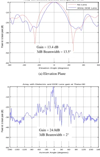
Figure 4-15: Slotted Waveguide Array Gain with Dielectric Lens and DOE Lens (d=0) (a) Elevation Plane (b) Azimuth Plane ……… 60

Figure 4-16: Slotted Waveguide Array Gain with only DOE Lens (d=0) (a) Elevation Plane (b) Azimuth Plane ……….. 61

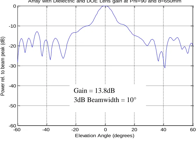
Figure 4-17: Slotted Waveguide Antenna Gain with Dielectric Lens and DOE Lens at d=650mm (a) Elevation Plane (b) Azimuth Plane ………...… 62

Figure 4-18: Slotted Waveguide Antenna Gain with only DOE Lens at d=650mm (a) Elevation Plane (b) Azimuth Plane ……….. 63

Figure 4-19: Difference Patterns for Slotted Waveguide Array with and without DOE Lens ……….. 65

Figure 5-1: Fabricated 10GHz DOE Lens ………... 66

Figure 5-2: Electric Field Measurement Setup ……… 67

Figure 5-3: Diagram of Image Formation Test ……… 68

Figure 5-4: Electric Field Intensity and Phase Distribution in the transmission plane of the DOE Lens at Varying Frequency using a Dipole ………..… 69

Figure 5-5: E-Field Magnitude along z-direction as it travels through center (Dipole 150mm from Lens) ……….. 70

Figure 5-6: E-Field Magnitude as it travels through the lens at various z distances in the transmission plane of the lens at 9.9GHz (Dipole 150mm from Lens) ………... 71

x | P a g e

Figure 5-8 E-Field Magnitude as it travels through the lens at various z distances in the

transmission plane of the lens at 10.1GHz (Dipole 150mm from Lens) ………. 73

Figure 5-9: Electric Field Measurement Setup with Horn Antenna ……… 74

Figure 5-10: Electric Field Intensity and Phase Distribution in the transmission plane of the DOE Lens at Varying Frequency using a Horn Antenna ………... 75

Figure 5-11: E-Field Magnitude along z-direction as it travels through center (Horn 250mm from Lens) ……….. 76

Figure 5-12: E-Field Magnitude as it travels through the lens at various z distances in the transmission plane of the lens at 9.9GHz (Horn 250mm from Lens) ……….. 77

Figure 5-13: E-Field Magnitude as it travels through the lens at various z distances in the transmission plane of the lens at 10GHz (Horn 250mm from Lens) ………... 78

Figure 5-14: E-Field Magnitude as it travels through the lens at various z distances in the transmission plane of the lens at 10.1GHz (Horn 250mm from Lens) ……… 79

Figure 5-15: Anechoic Chamber Setup ……… 80

Figure 5-16: Diagram of Anechoic Chamber Tests ………. 81

Figure 5-17: DOE Distance from Horn Antenna Vs. Rx Power ……….. 82

Figure 5-18: Horn Antenna Radiation Pattern with and without DOE Lens at 10GHz . 83 Figure 5-19: Gain vs Frequency Plot ………... 85

Figure 5-20: Gain Increase vs Frequency Plot ………. 85

Figure 5-21: Horn Antenna Radiation Pattern with and without DOE Lens at 8.6GHz . 86 Figure 5-22: Microstrip Patch Array ……… 87

Figure 5-23: DOE Distance from Patch Array Vs. Rx Power ………. 88

xi | P a g e

List of Tables

Table 3-1: 40GHz DOE Lens #1 Gain Enhancement ……….. 35

Table 3-2: 40GHz DOE Lens #2 Gain Enhancement ……….. 35

Table 3-3: Patch Array Gain Enhancement ………. 41

Table 4-1: Comparison of Simulated and C Speed Results ………. 46

Table 4-2: Slotted Waveguide Gain Enhancement ……….. 58

Table 4-3: Slotted Waveguide Array Gain Enhancement ……… 64

Table 5-1: Horn Antenna Power Enhancement with Fabricated DOE Lens …………... 82

Table 5-2: Horn Antenna Gain Enhancement across X-band ……….. 84

Table 5-3: Patch Array Power Enhancement with Fabricated DOE Lens ………... 88

Table 5-4: Overall Gain Enhancement ……….... 89

1 | P a g e

1 Introduction

1.1 Lens Antenna Overview

Lenses have been around for many years and have been used in the fields of

optics and electromagnetics. A lens has the ability to refract light or electromagnetic

radiation as it is transmitted through the lens. The lens can be used to either converge or

diverge the transmitted beam depending on the application. A lens is typically

characterized by its shape and the type of material it is made out of [1]. Some common

lenses are shown in figure 1-1.

2 | P a g e

Lenses have been used with antennas to shape to electromagnetic radiation into

the desired pattern. Depending on the type of lens and application, the radiation can be

focused to a certain point or spread out to cover a wider area. Lenses control the incident

radiation to prevent it from spreading in undesired directions [1]. A lens will also convert

the wave type through refraction. The three types of wavefronts are planar, cylindrical,

and spherical (Fig 1-2). A plane wave is a traveling wave which is emitted by a planer

source and consists of a plane surface parallel to the source [2]. The energy density for a

plane wave is constant so there is no attenuation and the amplitude remains constant. A

cylindrical wavefront is created from a line source and expands outward in a cylindrical

shape. As the distance from the line source increases the energy per unit area decreases.

A spherical wave is formed or collapses into a single point. A spherical wave expands to

fill the area of a sphere and therefore the energy density decreases according the r2 and the amplitude decreases according to the inverse of the radius [2].

(a) Planar (b) Cylindrical (c) Spherical

3 | P a g e

A simple or single refracting surface lens will have one surface act as the refractor

while the second surface will be non-refracting and match either the incoming or

outgoing wave type [3]. The diffraction caused by the refracting surface will determine

the new far-field pattern. The index of refraction is based upon the material of the lens

and is given by Equation (1-1)

r r

n   (1-1)

Lenses are more commonly utilized at higher frequency. At lower frequencies the

lens tends to be very large and heavy. Zoning the lens can help to reduce this problem.

Zoning reduces the size of the lens by removing multiples-of-wavelength path lengths

[3]. Zoning is done by stepping either the non-refracting or refracting surface of the lens.

Stepping the refracting surface causes some change in the field by diffracting the incident

wave. The dimensions for the steps can be calculated by equating the path length inside

and outside of the lens along the steps [3]. The step difference, is given by Eq (1-2)

1   

n



(1-2)

1.2 Dielectric Lenses

Dielectric lenses have been used for many years for all kinds of applications.

These applications include gain enhancement, beam scanning, beam shaping, and radar

applications. Dielectric lenses come in many different shapes which effect the diffraction

4 | P a g e

luneberg lens was first developed in 1944 by R.K Luneberg. The main characteristic of

the luneberg lens is that the index of refraction varies with the radius of the sphere [5].

The luneberg lens is used to focus an incoming wave into a point on the boundary of the

sphere which is opposite of the entry point. The lens is also able to form multiple beams

in arbitrary directions by moving the feed location around the lens [4]. A mirror or some

kind or radiator is usually placed at this focal point. The index of refraction in terms of

radius determines the path of the beam through the lens. Figure 1-3 shows the geometry

of a standard luneberg lens and in this case the index of refraction relates to the radius

according to equation 1-3 [5].

Figure 1-3: Geometry of a Standard Luneberg Lens [5]

2 2

2 r

n   (1-3)

There are many variations of the luneberg since the index of refraction inside the

5 | P a g e

the Maxwell fisheye, Eaton lens, and isotropic lens (Figure 1-4). The isotropic lens is

one of the more interesting variations as it returns the incoming wave in the same

direction it came from [5]

(a) (b)

Figure 1-4: Geometry of (a) Maxwell Fisheye and (b) Isotropic Lens [5]

Luneberg lenses are commonly used for various radar applications. These

applications include RCS augmentors, wide angle radar targeting, radar beacon and rapid

scanning systems [4, 5]. The downsides to the use of a luneberg lens are its size and

mechanical aspects.

6 | P a g e

While the luneberg lens is known for its varying index of refraction, most

dielectric lenses are made with a material with a constant dielectric constant. A common

hemispherical shaped dielectric lens was used with a patch array for wide angle

beam-scanning [6]. This lens was designed for 20GHz with a thickness of 57mm and diameter

of 200mm. The surface of the lens was designed by taking into account the refraction

law on the inner and outer surface, the energy conservation law, and Abbe’s sine

condition (1). One of the main problems they encounter was the residual phase delay

when scanning in the transverse plane. This problem was fixed by designing the patch

array to compensate for the phase delay and the beam scanning system was achieved

(Figure 1-6) [6].

7 | P a g e

Lenses are also commonly used to shape the beam of an antenna. In one case, an

RF lens is used to control and reduce the beamwidth of a directional antenna [7] for

direction of arrival estimation system. This is useful because the larger beamwidth may

interfere with the multiple paths in the system. The antenna being used was a four-arm

spiral antenna. Without making any changes to the physical structure of the antenna, the

RF lens is able to reduce its beamwidth [7]. The RF lens is bullet shaped and placed

directly on top of the antenna. Placing the dielectric RF lens directly on the antenna adds

the additional benefit of drawing more radiation towards to front. The RF lens was able

to successfully decrease the beamwidth of the antenna from 140° to 60° at 4GHz and

110° to 20° at 12GHz [7].

Figure 1-7: RF Bullet Lens with Spiral Antenna [7]

Many different dielectric lenses are used for gain enhancement. Gain

enhancement using a lens can allow the size of the antenna to be reduced and still

produce a good amount of gain. A hemispherical dielectric lens was used to enhance the

gain of a 4 element patch array at 2.7 GHz [8]. The lens has a diameter of 20cm and is

8 | P a g e

able to increase the gain of the 2x2 patch array by 4dB. The combination of the lens and

2x2 patch array resulted in a higher gain than that of a 2x4 patch array by itself and

therefore the size of the antenna can be reduced by using the lens [8].

Figure 1-8: Teflon Hemispherical Dielectric Lens [8]

A Fresnel lens is another type of dielectric lens that has been gaining popularity.

The Fresnel lens utilizes the zoning concept and has several zones to diffract the incident

beam. Many of the Fresnel lenses are flat while others used more of a curved shape. The

curved zone Fresnel lens has a very similar outline to the DOE lens. In 2011, a flat zone

Fresnel lens was designed for gain enhancement of a fractal antenna array at 24GHz [9].

The lens is a phase correcting zone plate lens with the radius of each zone found from

equation (1-4) where n is the number of zones, f is the focal length, and P is the number

of phases [9]. The lens is only 24mm by 24mm and made from CT765 LCC tape which

has a very high dielectric constant of 68.7. The lens was placed over the fractal array

9 | P a g e

2

2

       

P n P

nf

r o o (1-4)

Figure 1-9: Fresnel Lens and Fractal Array [9]

1.3 Metamaterial Lenses

In recent years metamaterial lenses have become very popular for enhancing the

performance of antennas and microwave circuits. Metamaterials exhibit properties that

are not found in nature and have to be artificially made. Many metamaterials have a

negative index of refraction unlike the dielectric lenses which have a positive index of

refraction. Metamaterials have the negative index of refraction because of the properties

of left-handed materials. A left handed-material has a negative permittivity and

permeability. When both the permittivity and permeability are plugged into the index of

refraction equation, it results in a negative value (eq 1-5) [9]. In a normal right-handed

material the Poynting vector and wave vector run parallel to each other. On the other

10 | P a g e

material [10]. Several metamaterial lenses have been built in the RIT Nanoplasmonics

and Metamaterials lab [10,…13].







n     *     (1-5)

A double-negative material (DNG) superstrate has been designed for gain

enhancement of a microstrip patch antenna [13]. The DNG superstrate is made by

drilling a triangular lattice of holes into a high dielectric slab. The DNG superstrate was

designed at 31GHz and exhibits an index of refraction of -1. Simulations of the DNG

superstrate proved the focusing properties of the metamaterial. After optimizing the

design of the DNG superstrate, a gain enhancement of 3.5dB was achieved [13].

Figure 1-10: Model of DNG Superstrate [13]

Another metamaterial that has been used for gain enhancement is the Zero-index

Metamaterial Lens (ZIML). The ZIML was designed to enhance the gain and directivity

of a 9.9GHz H-plane horn antenna and patch antenna [14]. The ZIML has a near zero

11 | P a g e

(ENZ) and a magnetic material with near zero permeability. A ZIM unit cell is created

with a modified split ring resonator using the magnetic material and a metal patch from

the electric material [14]. The ZIML can then be created using multiple ZIM unit cells.

The ZIML was able to reduce the beam width of the patch antenna from 123.5° to 31.2°

and increase its gain by 6.6dB. The lens was also able to enhance the gain of the H-plane

horn antenna by 4.43dB and reduce its beam width from 91.4° to 14.8°.

(a) (b)

Figure 1-11: (a) ZIM Unit Cell and (b) ZIML structure [14]

1.4 Motivation

Size and power are two of the main design choices for any antenna system. Often

there is tradeoff between these two as smaller antennas lead to a decrease in antenna gain

and therefore less power. For many years, engineers have been implementing different

types of lenses to deal with this tradeoff. By placing the lens in front of the antenna, the

12 | P a g e

motivation for this thesis came from working with a slotted waveguide antenna. The

single slotted waveguide antenna used a dielectric for gain enhancement and the results

from the HFSS model were very similar to what was expected. The slotted waveguides

were stacked to form an array to create the sum and difference patterns for radar

applications. The purpose of stacking the waveguides was to shape the beam in the

elevation plane. The resulting elevation beam did not shape as well as desired and

needed another focusing element. This thesis presents a new type of lens that has never

been used for antenna gain enhancement. The lens is called a Diffractive Optical

Element (DOE) lens which uses a series of curved zones to focus the radiated field,

enhance the gain, and shape the beam. The DOE lens is designed to be an add-on to

pre-existing antennas to improve their performance. The DOE lens has advantages over

previous lenses since it is lighter, thinner, and easily machined. The structure of the lens

is similar to a curved-zone plate Fresnel lens. These lenses have been used for other

applications like a photovoltaic concentrating system to increase the solar intensity on the

solar cell [15] and imaging and spectroscopy applications [16].

1.5 Major Contributions of Present Work

The present work presents the design of diffractive optical element (DOE) lens for

antenna gain enhancement and beam shaping.

The following summarizes the major contributions of the work.

1. A methodology has been developed for the design of a DOE lens, for different

13 | P a g e

has been tested in simulations. Lenses designed are for 10GHz and 40GHz horn

antennas, a 3 GHz slotted waveguide antenna array, and 10GHz microstrip patch

arrays. Beam shaping and focusing is clearly illustrated for each type of antenna.

Gain enhancement as high 20dB has been achieved for a 40-GHz horn antenna.

2. A comprehensive study of the slotted waveguide antenna with a dielectric lens has

been performed where the simulation results compare well the expected results. When

two of these antennas, each with a dielectric lens, are stacked as an array, the

elevation plane gain is low and the beam width too wide to be acceptable for radar

applications. A 3GHz DOE lens has been designed where a gain enhancement of 7dB

in the elevation plane has been achieved, as well as a decrease of the 3dB beamwidth

from 20° to 13.5°.

3. Experimental validation for the focusing properties and the gain enhancement has

been done. A 10 GHz DOE lens, made from rexolite, has been fabricated using CNC

milling. Image formation has been verified using an electric field probing station.

The electric field intensity in the transmission plane shows clearly the beam focusing

by the DOE lens. Radiation and gain measurements in an anechoic chamber show a

gain enhancement of 6.6 dB for the horn antenna and of 5.6 dB for the patch array.

1.6 Organization of Present Work

This work has been divided into 5 chapters. The first chapter is an introduction

14 | P a g e

metamaterials lenses that have been previously used for gain enhancement. Chapter 2 is

a walkthrough of the design and analysis of the DOE lens. It explains how the DOE lens

structure was developed and shows the focusing properties of the lens. Chapter 3

presents the simulation results showing the gain enhancement of the DOE lenses. The

chapter provides a detailed analysis of the DOE lens simulations with different antennas

and frequencies. The fourth chapter gives an overview and analysis of the slotted

waveguide antenna with the dielectric lens. The DOE lens is placed with the slotted

waveguide and the results are analyzed. Chapter 5 explains the experimental validation

that was performed to test the 10GHz DOE lens. An electric field probing station and

RIT’s anechoic chamber are used to verify focusing of the lens and gain enhancement.

15 | P a g e

2 Design and Analysis of a DOE Lens

DOE lens (Diffractive Optical Element) focuses light through constructive

interference and diffraction to focus energy at a certain focal length. It is composed of a

series of zones. The lens in figure 2.1 has 5 zones which includes the center curvature of

the lens. The phase is the same everywhere on each zone at the focal point. The phase

difference between neighboring zones is 2π. This gives a constructive interference at the

focus. The zones are used to decrease the size of the lens and reduce the number of

elements needed in a lens system. The zones of the lens become finer towards the edge

of the lens [17].

Figure 2-1: Contour of a DOE Lens

T

Focal Length (f)

Ts

16 | P a g e

The structure of the lens is created from the optical path length (eq 2-1) where n is

the refractive index, f is the focal length, and y is the height at a certain point on the lens.

To design the contour of the lens, the z value must be obtained for every value of y. This

is done by manipulating the optical path length (2-1) into the form of a quadratic equation

with z being the unknown variable. The optical path length is the total distance traveled

by the wave in the lens and in free space multiplied by the respective refractive index.





0 nz y f z

L     (2-1)

At any height y, 1st term is the distance travelled in the lens times the refractive

index ‘n’ and the 2nd term is the distance traveled in FS which is the hypotenuse where f

is measured including center thickness ‘T’ times the refractive index of one.

Manipulate Eq 2-1 to create the quadratic equation:



 



0 2 z f nz L

y    

2 2 2 2 0 2 0 2 2

2L n z f fz z

L

y      













Eq 2-2 is a quadratic equation (az2+bz+c=0) where a













0 f y

L

c   . The contour of the DOE lens is defined by solving for the quadratic

equation (Eq 2-3)



 













17 | P a g e

On the axis (y=0), where z = T





nT

L₀    (2-4)

With the phase difference as 2π

 

L0   (2.5)

Since eq (2.5) is valid for all values of f,

1 -n Tmax



 (2.6)

The lens should focus the radiation into a focal point at the focal length. The

focal point is the area where the radiation from the lens arrives at an equal phase [16].

The lens must be designed so that the phase at the focal point is independent of the path

length. It is important to take into account the phase especially for zoned lenses like the

DOE lens. Zoning a lens progressively increases its thickness to a certain point then goes

back to zero and repeats the process. This causes frequency dependence since the path

lengths have changed. In order for the phase change not to be altered across the zones,

the path length must be changed in multiples of a wavelength [17]. As seen in figure 2-1,

the DOE lens has zones that are placed so the optical path length varies in multiples of

one wavelength causing a 2π difference in phase across each. Therefore the phases will

be equal at the focal point. Each zone forces the field to travel through different

thicknesses of the dielectric so the phase will be properly adjusted as it leaves the lens

18 | P a g e

A matlab code has been generated to create the profile of the DOE lens by

entering the necessary design parameters. The design parameters are the thickness (T),

the index of refraction (n), the wavelength at the desired frequency (λ), the slab thickness

(Ts), and the focal length (f). Using these design parameters the code uses eq 2-3 to

create the profile of the lens for values of y extending to infinity. The diameter, D, can

be selected to create the actual lens design. The selection for a reasonable value for D is

made relative to the size of the antenna that the lens will be used for. Choosing the

diameter will not affect the profile of the lens, it will just determine the number of zones

that are included in the design. When y=0 in eq 2-3, the corresponding z value will equal

the thickness, T. If y =D/2, then z equals the thickness at the edge of the lens. The lens

in figure 2-1 is considered to have 5 zones that include the center. The focal length is the

design parameter that has the largest effect on the contour of the DOE lens at a particular

frequency (Figure 2-2). Each plot in figure 2-2 has the same parameters T, Ts, D, n, and

frequency, except for the focal length. A smaller focal length will create more zones

within a given diameter, D, while a larger focal length will have less zones but a more

dominant center zone. If the lens is being designed for a fixed diameter then the focal

length can be changed to include a specific amount of zones in the lens design. Once the

contour of the lens is generated in MATLAB, a MATLAB-to-HFSS-API is used to model

the DOE lens in HFSS. The lens is then imported into CST Microwave Studio to

19 | P a g e

(a) f = 50mm (b) f = 150mm

(c) f = 200mm (d) f = 300mm

Figure 2-2: Cross Section of DOE Lens with Varying Focal Length, f (Freq =40GHz, D=225mm, T=11.4mm, Ts=14.3mm, n=1.6)

Figure 2-3: CST Microwave Studio DOE Lens

-0.1 -0.05 0 0.05 0.1 0.15 -0.1 -0.08 -0.06 -0.04 -0.02 0 0.02 0.04 0.06 0.08 0.1

40GHz DOE with 50mm Focal Length

x (mm) y ( m m )

-0.1 -0.05 0 0.05 0.1 0.15

-0.1 -0.08 -0.06 -0.04 -0.02 0 0.02 0.04 0.06 0.08 0.1

40GHz DOE with 150mm Focal Length

x (mm)

y

(m

m

)

-0.1 -0.05 0 0.05 0.1 0.15

-0.1 -0.08 -0.06 -0.04 -0.02 0 0.02 0.04 0.06 0.08 0.1

40GHz DOE with 200mm Focal Length

x (mm) y ( m m )

-0.1 -0.05 0 0.05 0.1 0.15 -0.1 -0.08 -0.06 -0.04 -0.02 0 0.02 0.04 0.06 0.08 0.1

40GHz DOE with 300mm Focal Length

x (mm) y ( m m ) z (mm) z (mm) z (mm) z (mm)

40GHz DOE with 50mm Focal Length

40GHz DOE with 200mm Focal Length

40GHz DOE with 150mm Focal Length

20 | P a g e

The diffractive optical element (DOE) lens is designed to focus the

electromagnetic energy that passes through it. The energy should converge into a single

point at the lens’s focal length. The focusing properties of the DOE lens have been

investigated by a plane wave excitation. The plane wave is excited 50mm from the edge

of the DOE lens. The electric field magnitude in the center (y=0) along the Z-direction is

plotted (Figure 2-4). This plot shows that the energy converges to a maximum at

146mm. This is slightly shorter than the lens’s focal length of 168mm. The 2D E-field

magnitude in the XZ and YZ plane is shown in figure 2-5. As expected the magnitude in

the two planes are the same due to the symmetry of the lens.

Figure 2-4: E-Field Magnitude along Z-direction

-50 0 50 100 150 200 250

0 0.5 1

Y Length (mm)

E

z

Fi

el

d

M

ag

ni

tu

de

Ez(mag) along Y-Direction (center)

-250 -200 -150 -100 -50 0 50

-200 -100 0 100 200

Y Length (mm)

P

ha

se

(D

eg

re

es

)

Transmitted Ez(phase) along Y-Direction (center)

E-Field Mag along Z-Direction (center)

21 | P a g e

(a) XZ Plane

(b) YZ Plane

Figure 2-5: 2D E-Field Magnitude in (a) XZ Plane (b) YZ Plane Z

X

22 | P a g e

The focusing properties of a 10GHz DOE lens have been shown using a dipole

antenna as the source. The electric field magnitude and phase distribution in the

transmission plane of the lens can be seen in figure 2-6. Figure 2-7 shows the electric

field magnitude along the z direction at the center zone of the lens. The focal point is at

63mm, which again is slightly shorter than the designed focal length of 85mm. The

electric field was also plotted across the y direction at various z distances as shown in

figure 2-8. It can be seen that the highest electric field magnitude is for z=65mm. The

electric field stays close to the maximum when z is at 60mm and 70mm, but then drops

off as z moves further from the maximum. These figures show how the maximum is

focused in the center of the lens as expected and the electric field magnitude quickly

23 | P a g e

(a) Magnitude

(b) Phase

Figure 2-6: Electric Field Magnitude and Phase Distribution of a 10GHz DOE Lens z Dimension (mm)

y D im e n si o n ( m m )

E-Field Magnitude (V/m)

-50 0 50 100 150 200 250 300

-100 -80 -60 -40 -20 0 20 40 60 80 100 1 2 3 4 5 6 7 8 9 10

z Dimension (mm)

y D im e n si o n ( m m ) Phase (degrees)

-50 0 50 100 150 200 250 300

24 | P a g e

Figure 2-7: E-Field Magnitude along z-direction through center zone (Dipole 150mm from Lens)

-50 0 50 100 150 200 250 300

0 0.1 0.2 0.3 0.4 0.5 0.6 0.7 0.8 0.9 1

y Length (mm)

E

z

F

ie

ld

M

ag

n

it

u

d

e

E-Field Magnitude along z-direction as it travels through center zone (Dipole 150mm from Lens)

25 | P a g e

Figure 2-8: E-Field Magnitude as it travels through the lens at various z distances in the transmission plane of the lens at 10GHz (Dipole 150mm from Lens)

-1000 -80 -60 -40 -20 0 20 40 60 80 100

1 2 3 4 5 6 7 8 9 10

y length (mm)

E

-F

ie

ld

M

ag

ni

tu

de

(

V

/m

)

E-Field Magnitude as it travel through the lens at various z distances in the transmission plane of the lens at 10GHz (Dipole 150mm from Lens)

26 | P a g e

3 Gain Enhancement using the DOE Lens

3.1 DOE Lens at 40GHz with Horn Antenna

The DOE lens used for the initial testing has been designed at 40GHz (figure 3-1)

where n=1.6, for a focal length f=168.75 mm and a chosen diameter D=225mm, slab

thickness Ts=14.3 mm, and zone thickness, T=11.4 mm. The diameter of the DOE lens

allows five zones to be included in the final design. This lens will be referred to as

40GHz Lens #1 throughout this thesis.

Figure 3-1: 40GHz DOE Lens #1 (a) Contour (b) 3-D Model

A second 40GHz lens that has also been modelled to compare to this first 40GHz

DOE lens is much smaller. The focal length was decreased in order to get the same

number of zones in the lens with a smaller diameter. This lens, seen in figure 3-2 has

been designed with the parameters of n=1.6, diameter D=90 mm, focal length f=11.25

mm, slab thickness Ts=14.3 mm, and zone thickness, T=11.4 mm. This lens also has five

zones and will be referred to 40GHz DOE Lens #2.

-0.1 -0.05 0 0.05 0.1 0.15 -0.1

-0.08 -0.06 -0.04 -0.02 0 0.02 0.04 0.06 0.08 0.1

40GHz DOE Lens

x (m)

y

(m

)

z (m) 225mm

27 | P a g e

Figure 3-2: Contour of 40GHz DOE Lens #2

The antenna used for simulation purposes is a 40GHz horn antenna with a model

available in CST (figure 3-3). The 40GHz horn antenna is 14.7mm x 16.7mm with a gain

of 15.4dB and half power beamwidth of 29° (figure 3-4). The DOE lens is simulated by

placing it in front of the horn antenna and varying the distance, d as shown in figure 3.6.

There is an optimal distance, d at which gain enhancement is a maximum.

-0.03 -0.02 -0.01 0 0.01 0.02 0.03 0.04 0.05 0.06 0.07 -0.04

-0.03 -0.02 -0.01 0 0.01 0.02 0.03 0.04

Smaller 40GHz DOE Lens

x (m)

y(

m

)

z (m) 90mm

28 | P a g e

Figure 3-3: 40GHz Horn Antenna

Figure 3-4: 40GHz Horn Antenna Gain

-180 -120 -60 0 60 120 180

-40 -30 -20 -10 0 10 20

40GHz Horn Antenna Gain

Theta (Degrees)

G

ai

n

(d

B

)

14.7mm

16.7mm

Gain =15.4 dB

3dB Beamwidth = 29° 40GHz Horn Antenna Gain

29 | P a g e

Figure 3-5: 40GHz Horn Antenna 3D Polar Plot

30 | P a g e

The simulation results show substantial gain enhancement and beam shaping

when the lens is placed in front of the antenna. The gain of only the horn antenna

without the lens is 15.4dB compared to 35.5dB when the DOE lens is placed at an

optimal distance d=118.6mm in front of the antenna resulting in a gain enhancement of

20.1dB. As seen in figure 3-7 the DOE lens has shaped the beam significantly. The

3dBbandwidth decreases from 29° to 2.3° when the DOE lens is used. Table 3-1 shows

the gain enhancement as the distance of the DOE lens #1 is varied. The gain will increase

as the lens is moved closer to the optimal distance and then decrease as the lens continues

to move past it. The 2D electric field magnitude, figure 3-8, shows the radiated energy

converging around the focal length. As expected the electric field in the YZ and XZ are

symmetric due to the symmetry of the DOE lens. The 40GHz DOE Lens #1 shows a

very large gain enhancement however the lens diameter of 225mm is much larger

compared to the size of the horn antenna which is 14.7mm x 16.7mm. The 40GHz DOE

Lens #2 is simulated in the same way as the first lens and also displays a considerable

gain enhancement. At an optimal distance of 140mm, the DOE lens increases the gain of

the horn antenna from 15.4dB to 25.6dB (figure 3-9). Even though this enhancement of

10.2dB is lower as compared to that of DOE Lens #1, still it is very good. The beam is

again sharpened and has a 3dB beamwidth of 4.2°. Table 3-2 shows the gain

enhancement as the distance of the lens is varied and shows a similar trend to DOE lens

#1. This shows that the level of gain enhancement is directly related to the size of the

DOE lens. When designing one of these lenses it is important to consider the tradeoff

31 | P a g e

(a)

(b)

Figure 3-7: (a) Gain and (b) 3D Polar Plot of 40GHz Horn Antenna with DOE Lens #1 at d=118.6mm

-180 -120 -60 0 60 120 180

-40 -30 -20 -10 0 10 20 30 40

Theta (degrees)

G

ai

n

(d

B

)

40GHz Horn Antenna with and without 40GHz DOE Lens#1 40GHz DOE Lens #1 No Lens

Gain = 35.5 dB

32 | P a g e

(a) YZ Plane

(b) XZ Plane

33 | P a g e

(a)

(b)

Figure 3-9: (a) Gain and (b) 3D Polar Plot of 40GHz Horn Antenna with DOE Lens #2 at d=140mm

-180 -120 -60 0 60 120 180

-40 -30 -20 -10 0 10 20 30 40

Theta (degrees)

G

ai

n

(d

B

)

40GHz Horn Antenna with and without 40GHz DOE Lens #2

40GHz DOE Lens #2 No Lens

Gain = 25.5 dB

34 | P a g e

(a) YZ Plane

(b) XZ Plane

35 | P a g e

Table 3-1: 40GHz DOE Lens #1 Gain Enhancement

Distance (d) Gain Gain increase

98.6 mm 30.6 dB 15.2 dB

108.6mm 33.8 dB 18.4 dB

113.1 mm 35 dB 19.6 dB

116.1 mm 35.2 dB 19.8 dB

118.6 mm 35.5 dB 20.1 dB

121.1 mm 35.4 dB 20 dB

126.1 mm 34.7 dB 19.3 dB

136.1 mm 31.3 dB 15.9 dB

Table 3-2: 40GHz DOE Lens #2 Gain Enhancement

Distance (d) Gain Gain increase

118.5 mm 24.2 dB 8.8 dB

128.5 mm 25.0 dB 9.6 dB

138.5 mm 25.5 dB 10.1 dB

140 mm 25.6 dB 10.2 dB

143.5 mm 25.5 dB 10.1 dB

148.5 mm 25.5 dB 10.1 dB

158.5 mm 24.9 dB 9.5 dB

3.2 DOE Lens at 10GHz with Horn Antenna

The next DOE lens is the one designed at 10GHz and used in the experimental

validation with measurements in RIT’s ETA (Electromagnetic Theory and Application)

Lab anechoic chamber. The design parameters for this lens are n=1.6, diameter D=280

mm, focal length f=85 mm, slab thickness Ts=12.5 mm, and zone thickness, T=35 mm.

The choice for D is based on the commercially available block of rexolite (304.8mm x

36 | P a g e

diameter of 280mm to fit the size of the block. The focal length is chosen to be 85mm so

that three zones would be included in the final design shown in figure 3-11.

Figure 3-11: Contour of 10GHz DOE Lens

The 10GHz DOE lens is used with a 10GHz horn antenna (67.63mm x 76.83mm)

that has the same radiation characteristics as the 40GHz horn (figure 3-4). A gain

enhancement of 8.1dB at the optimal distance of 380mm is achieved. This is a

significant gain enhancement considering the size of the lens is comparable to that of the

antenna.

-0.1 -0.05 0 0.05 0.1 0.15

-0.1 -0.05 0 0.05 0.1

10GHz DOE Lens

y

(m

)

z (m)

280mm

10GHz DOE Lens

37 | P a g e

Figure 3-12: Gain of 10GHz Horn Antenna with DOE Lens at d=380mm

3.3 DOE Lens at 10GHz with Microstrip Patch Array

A 10GHz micro-strip patch array has also been used with the 10GHz DOE lens to

show the lens could work with different antennas. A 2x2 (60mm x 44mm) and 3x3

(90mm x 66mm) patch array were simulated with the patches in-phase. The CST model

for the 2x2 array is shown in figure 3-13. The gain of the 2x2 patch array is 14.4dB with

a 3dB beamwidth of 26° (figure 3-14). Figure 3-15 shows the gain enhancement and

beamshaping from the DOE lens when it is placed the optimal distance, d=480mm. The

DOE lens enhances the gain 9.6dB to 24dB and decreases the 3dB beamwidth to 5°.

-180 -120 -60 0 60 120 180

-25 -20 -15 -10 -5 0 5 10 15 20 25

Theta (degrees)

G

ai

n

(d

B

)

10GHz Horn Antenna with and without 10GHz DOE Lens

10GHz DOE Lens No Lens

38 | P a g e

Figure 3-13: 2x2 Microstrip Patch Array Model

Figure 3-14: Gain of 10GHz 2x2 Patch Array

-180 -120 -60 0 60 120 180

-25 -20 -15 -10 -5 0 5 10 15 20

Theta (degrees)

G

a

in

(

d

B

)

Radiation Pattern of 2x2 Patch Array

Gain =14.4 dB

3dB Beamwidth = 26° 60mm

15mm

Radiation Pattern of 2X2 Patch Array

39 | P a g e

Figure 3-15: Radiation Pattern of 10GHz 2x2 Patch Array with and without DOE Lens

The 3x3 patch array (90mmx66mm) that has been tested with the lens had an

original gain of 17.8dB and a beamwidth of 23°. This is a higher gain and thinner

beamwidth than the 2x2 array. When the DOE lens was placed at an optimal distance of

480mm the gain increased to 23.7dB and the beamwidth reduced to 5° (figure 3-18). The

gain is still lower than that of the 2x2 patch array when the DOE lens was used.

-180 -120 -60 0 60 120 180

-25 -20 -15 -10 -5 0 5 10 15 20 25

Theta (degrees)

G

a

in

(d

B

)

Radiation Pattern of 2X2 Patch Array with and without DOE Lens

DOE Lens No DOE Lens

Gain = 24 dB

40 | P a g e

Figure 3-16: 3x3 Microstrip Patch Array Model

Figure 3-17: Gain of 10GHz 3x3 Patch Array

-180 -120 -60 0 60 120 180

-25 -20 -15 -10 -5 0 5 10 15 20

Theta (degrees)

G

a

in

(

d

B

)

Radiation Pattern of 3x3 Patch Array

Gain =17.8 dB

3dB Beamwidth = 23° Radiation Pattern of 3X3 Patch Array

Theta (degrees) 90mm

41 | P a g e

Figure 3-18: Radiation Pattern of 10GHz 3x3 Patch Array with and without DOE Lens

Table 3-3: Patch Array Gain Enhancement

Gain Gain Increase

2x2 Patch Array 14.4 dB

9.6 dB

2x2 Patch Array with DOE Lens at d=480mm 24.0 dB

3x3 Patch Array 17.8 dB

5.9 dB

3x3 Patch Array with DOE Lens at d=380mm 23.7 dB

The 10GHz DOE lens was able to enhance the gain of both formations; however

the gain increase for the 2x2 array was much greater. This was expected since the beam

of the 3x3 array was sharper than that of the 2x2 array. This means that instead of

designing a higher order patch array, a DOE lens can be designed to be used with a lower

order array and still produce the same gain. These results show that the fabricated 10GHz

DOE lens should enhance the gain of multiple types of antennas.

-180 -120 -60 0 60 120 180

-25 -20 -15 -10 -5 0 5 10 15 20 25

Theta (degrees)

G

ai

n

(d

B

)

Radiation Pattern of 3X3 Patch Array with and without DOE Lens DOE Lens No DOE Lens

42 | P a g e

4 Slotted Waveguide Antenna

A marine radar antenna comprises of a slotted waveguide, where the slots open

into side horn plates [20]. For size reduction, narrow beam within the elevation plane and

enhanced gain, a polarization grid, and a dielectric filled radome have been placed in

front of the antenna. The motivation for this work came when analyzing a slotted

waveguide antenna that used a dielectric lens (figure 4.1) for beamshaping and gain

enhancement. When the antenna was modeled in HFSS the results almost matched the

expected results that were given. The single slotted waveguide has a very focused beam

that works well for radar applications. However, the purpose of the slotted waveguide

was to stack them as a two-element array in order to form the sum and difference patterns

in the elevation plane for radar applications. When stacked the beamwidth of the

elevation plane was still large and the gain low. Another focusing element was needed to

improve the antenna performance in the elevation plane. The DOE lens has been

designed to shape the beam in the elevation plane and enhance the gain.

4.1 Single Slotted Waveguide with Dielectric Lens

Figure 4-1: HFSS Antenna Model Bottom Side

Horn Plate

Top Side Horn Plate

Dielectric Lens Polarization Grid

43 | P a g e

The slotted waveguide antenna uses two side plates and a polarization grid to

direct the radiation towards the dielectric lens which is used for gain enhancement. The

simulations have been performed at 3 GHz. The material of the slotted waveguide was set

to PEC (perfect electric conductor) and the outer faces of the slotted waveguide were

given a boundary condition of perfect E. The perfect E boundary represents a perfectly

conducting surface. The left end of the slotted waveguide was excited using a wave port.

The wave port represents the location where the excitation signal enters the structure. In

order to ensure no reflections, the other end of the slotted waveguide is terminated by a

matched load, of value equal to the intrinsic impedance, ZTE10, of the dominant TE10

mode in propagating in the guide. The impedance ZTE10 is calculated using eq. (4-1)

where fc10 is the cutoff frequency of the mode. This is represented in HFSS using an

impedance boundary set equal to ZTE10 = 523.93Ω. The simulations show the waveguide

is operating in the TE10 as expected. The electric field is parallel to the shorter side of

the waveguide (fig 4-2a) and the wave is propagating at an operating frequency of 3GHz

since the waveguide cutoff frequency is 2GHz (fig 4-2b). The phase constant can also be

calculated (eq 4-3). The radiation box was set to be a distance of λo/4 from each edge of

the waveguide and the outer faces of the box were assigned a radiation boundary.

1

Z

2

10 ) (

TE

       

f

fc

o



(4-1)

a c fc

2

44 | P a g e f f 1 β 2 c10 (o) TE10          (4-3) where r o r o o       _        2 ) ( (4-4)

And εr equals the dielectric constant of the region within the waveguide. With a = 72mm,

fc10 = 2.08GHz.

(a)

(b)

Figure 4-2: (a) TE10 Mode E-Field Configuration and (b) Waveguide Propagation

0 1 2 3 4 5 6 7 8 9 10

0 50 100 150 200 250

Slotted Waveguide Propagation

45 | P a g e

Figure 4-3: HFSS Antenna Model Side View

The final component of the antenna is the dielectric lens which is placed in front

of the slotted waveguide and polarization grid. The dielectric lens is made out of a

foamed plastic like PVC. The manufacturing data for PVC shows the dielectric constant

for this material is between 1.6 and 2. For the simulation, the dielectric lens was initially

assigned a dielectric constant value of 1.6. The dielectric lens was placed 54mm in front

of the polarization grid. The full antenna model is shown in figure 4-3.

Figures 4-4 through 4-5 compare the simulation results with those provided by C

Speed for the full antenna. The dielectric constant of the dielectric lens was set to 1.6 for

the simulation results. The simulation and expected results compare very well with each

other. The one noticeable difference is the level of the sidelobe at 33°. The simulation

results show the sidelobe level to be -20dB while the expected results show the sidelobe

to be closer to -40dB. We cannot be sure that the simulation sidelobe levels are incorrect 54mm

Polarization Grid Slotted

Waveguide _{Dielectric Lens}

Top Side Horn Plate

46 | P a g e

until a far field test is performed. The expected results provided by C Speed are near

field results that have been converted to far field. The data is summarized in table 4-1.

Table 4-1: Comparison of Simulated and C Speed Results

Directive Gain Main Beam Angle Half-Power

Beamwidth

Simulated C Speed Simulated C Speed Simulated C Speed

Azimuth

Plane 25.8 dB 28.7 dB -5° -3.83° 2° 1.91°

Elevation

47 | P a g e

(a)

(b)

Figure 4-4: Elevation Plane Radiation Patterns for Complete Antenna System

(a) Simulated Results in CST (b) C Speed Results

-60 -40 -20 0 20 40 60

-60 -50 -40 -30 -20 -10 0

Elevation Angle (degrees)

P

ow

er

re

l.

to

b

ea

m

p

ea

k

(d

B

)

Slotted WG with Dielectric Lens gain at Phi=90

48 | P a g e

(a)

(b)

Figure 4-5: Azimuth Plane Radiation Patterns for Complete Antenna System

(a) Simulated Results in CST (b) C Speed Results

-180 -150 -120 -90 -60 -30 0 30 60 90 120 150 180

-60 -50 -40 -30 -20 -10 0

Azimuth Angle (degrees)

P

ow

er

re

l.

to

b

ea

m

p

ea

k

(d

B

)

Slotted WG with Dielectric Lens gain at Theta=90

49 | P a g e

4.2 Array of Slotted Waveguide Antennas with two Dielectric Lenses

The array is created by duplicating the antenna. The duplicated antenna was

placed a distance ‘d’ above the original antenna. The top antenna was excited the same

way as the bottom antenna. . Figures 4-7 show the radiation patterns for the array when

the spacing is 11.5cm. The results for the array are very promising and show a gain

increase of about 2dB. The array showed an increase in gain from 25.8dB to 27.8dB.

The results also showed very little interference from mutual coupling. Simulating the

array with different spacing had a minimal effect on the radiation patterns (appendix A).

Figure 4-6: Two Element Array of Complete Antenna System

Antenna #2

Antenna #1

d Dielectric Lens

Polarization Grid

Slotted Waveguide

50 | P a g e

(a)

(b)

Figure 4-7: CST Simulation Results for Array of Complete Antenna System (Spacing 11.5cm) (a) Elevation Plane (b) Azimuth Plane

-90 -60 -30 0 30 60 90

-60 -50 -40 -30 -20 -10 0

Elevation Angle (degrees)

P ow er r el . to b ea m p ea k (d B )

Array for Complete Antenna System

-180 -150 -120 -90 -60 -30 0 30 60 90 120 150 180

-60 -50 -40 -30 -20 -10 0

Azimuth Angle (degrees)

P ow er r el . to b ea m p ea k (d B )

Array for Complete Antenna System

Gain = 27.8dB 3dB Beamwidth = 2° Gain = 6.7dB

51 | P a g e

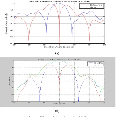
Figure 4-8 shows the sum and difference patterns in the elevation and azimuth

planes for the array on the same plot. The sum pattern is created when the two antennas

are in phase and the difference pattern is created when the antennas were 180° out of

phase. The difference pattern is only created in the elevation plane since that is the plane

the array was setup in. As expected there is a sharp null at 0° in the elevation plane. In

the azimuth plane the difference pattern is a constant line at -200dB due to the null

52 | P a g e

(a)

(b)

(c)

Figure 4-8: CST Difference and Sum Patterns for Spacing 11.5cm (a) Elevation Plane (b) C Speed Elevation Plane (b) Azimuth Plane

-90 -60 -30 0 30 60 90

-60 -50 -40 -30 -20 -10 0

Elevation Angle (degrees)

Po we r r el. to b ea m p ea k (d B)

Sum and Difference Patterns for spacing of 11.5cm

Difference Sum

-180 -150 -120 -90 -60 -30 0 30 60 90 120 150 180

-220 -200 -180 -160 -140 -120 -100 -80 -60 -40 -20 0

Azimuth Angle (degrees)

Po we r r el. to b ea m p ea k (d B)

53 | P a g e

4.3 DOE Lens for the Single Slotted Waveguide Antenna

The formation of the array did help to shape the beam in the elevation plane, but

not as much as desired. Another focusing element was needed to enhance the beam in

the elevation plane so a 3GHz DOE lens has been designed. The parameters for this lens

are n=1.6, diameter D=600 mm, focal length f=125 mm, slab thickness Ts=12.5 mm, and

zone thickness, T=90 mm (Figure 4-9).

Figure 4-9: Contour of 3GHz DOE Lens

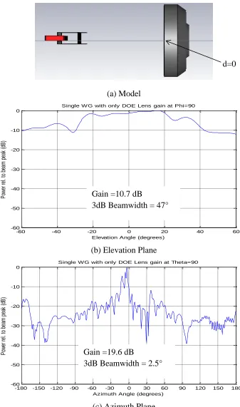
The DOE lens was put directly after the dielectric lens (d=0) while it was still in

place and was first tested with a single slotted waveguide (figure 4-10a). The dielectric

lens is then removed while the DOE lens is still held at d=0 (figure 4-11a). The 3GHz

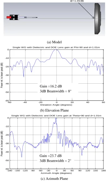
DOE lens was also placed farther away from the dielectric lens to see if the gain can be

enhanced even further. The DOE lens is placed at an optimal distance (1.01m) from the

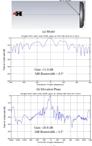
dielectric lens (figure 4-12a). The dielectric lens is then removed and the DOE lens is

kept at d=1.01m (figure 4-13a).

-0.3 -0.2 -0.1 0 0.1 0.2 0.3 0.4

-0.25 -0.2 -0.15 -0.1 -0.05 0 0.05 0.1 0.15 0.2 0.25

3GHz DOE Lens

y

(m

)

z (m)

54 | P a g e

(a) Model

(b) Elevation Plane

(c) Azimuth Plane

Figure 4-10: Slotted Waveguide Antenna Gain with Dielectric Lens and DOE Lens (d=0) (a) Model (b) Elevation Plane (c) Azimuth Plane

-60 -40 -20 0 20 40 60

-60 -50 -40 -30 -20 -10 0

Elevation Angle (degrees)

P ow er re l. to b ea m p ea k (d B )

Single WG with Dielectric and DOE Lens gain at Phi=90

-180 -150 -120 -90 -60 -30 0 30 60 90 120 150 180

-60 -50 -40 -30 -20 -10 0

Azimuth Angle (degrees)

P ow er re l. to b ea m p ea k (d B )

Single WG with Dielectric and DOE Lens gain at Theta=90

Gain =22.2 dB 3dB Beamwidth = 2° Gain =13.0 dB

3dB Beamwidth = 30.5° 490 mm

271 mm

592.5 mm

55 | P a g e

(a) Model

(b) Elevation Plane

(c) Azimuth Plane

Figure 4-11: Slotted Waveguide Antenna Gain with only DOE Lens (d=0) (a) Model (b) Elevation Plane (c) Azimuth Plane

-60 -40 -20 0 20 40 60

-60 -50 -40 -30 -20 -10 0

Elevation Angle (degrees)

P ow er re l. to b ea m p ea k (d B )

Single WG with only DOE Lens gain at Phi=90

-180 -150 -120 -90 -60 -30 0 30 60 90 120 150 180

-60 -50 -40 -30 -20 -10 0

Azimuth Angle (degrees)

P ow er re l. to b ea m p ea k (d B )

Single WG with only DOE Lens gain at Theta=90

Gain =19.6 dB

3dB Beamwidth = 2.5° Gain =10.7 dB

3dB Beamwidth = 47°

56 | P a g e

(a) Model

(b) Elevation Plane

(c) Azimuth Plane

Figure 4-12: Slotted Waveguide Antenna Gain with Dielectric Lens and DOE Lens at d=1.01m (a) Model (b) Elevation Plane (c) Azimuth Plane

-60 -40 -20 0 20 40 60

-60 -50 -40 -30 -20 -10 0

Elevation Angle (degrees)

P ow er re l. to b ea m p ea k (d B )

Single WG with Dielectric and DOE Lens gain at Phi=90 and d=1.01m

-180 -150 -120 -90 -60 -30 0 30 60 90 120 150 180

-60 -50 -40 -30 -20 -10 0

Azimuth Angle (degrees)

P ow er re l. to b ea m p ea k (d B )

Single WG with Dielectric and DOE Lens gain at Theta=90 and d=1.01m

Gain =23.7 dB 3dB Beamwidth = 2° Gain =16.2 dB 3dB Beamwidth = 8°

57 | P a g e

(a) Model

(b) Elevation Plane

(c) Azimuth Plane

Figure 4-13: Slotted Waveguide Antenna Gain with only DOE Lens at d=1.01m (a) Model (b) Elevation Plane (c) Azimuth Plane

-60 -40 -20 0 20 40 60

-60 -50 -40 -30 -20 -10 0

Elevation Angle (degrees)

P ow er re l. to b ea m p ea k (d B )

Single WG with only DOE gain at Phi=90 and d=1.01m

-180 -150 -120 -90 -60 -30 0 30 60 90 120 150 180

-60 -50 -40 -30 -20 -10 0

Azimuth Angle (degrees)

P ow er re l. to b ea m p ea k (d B )

Single WG with only DOE gain at Theta=90 and d=1.01m Gain =11.0 dB

3dB Beamwidth = 8.5°

Gain =20.8 dB

58 | P a g e

Table 4-2 summarizes the results for the different configurations of lenses for a