Characterising linear spatio-temporal dynamical systems in the frequency domain

This is a repository copy of Characterising linear spatio-temporal dynamical systems in the

frequency domain.

White Rose Research Online URL for this paper:

http://eprints.whiterose.ac.uk/74603/

Monograph:

Billings, S.A. and Wei, H.L. (2007) Characterising linear spatio-temporal dynamical

systems in the frequency domain. Research Report. ACSE Research Report no. 944 .

Automatic Control and Systems Engineering, University of Sheffield

[email protected] https://eprints.whiterose.ac.uk/

Reuse

Unless indicated otherwise, fulltext items are protected by copyright with all rights reserved. The copyright exception in section 29 of the Copyright, Designs and Patents Act 1988 allows the making of a single copy solely for the purpose of non-commercial research or private study within the limits of fair dealing. The publisher or other rights-holder may allow further reproduction and re-use of this version - refer to the White Rose Research Online record for this item. Where records identify the publisher as the copyright holder, users can verify any specific terms of use on the publisher’s website.

Takedown

If you consider content in White Rose Research Online to be in breach of UK law, please notify us by

Characterising Linear Spatio-Temporal Dynamical

Systems in the Frequency Domain

S.A. Billings and H.L. Wei

Research Report No. 944

Department of Automatic Control and Systems Engineering

The University of Sheffield

Mappin Street, Sheffield,

S1 3JD, UK

Characterising Linear Spatio-Temporal Dynamical

Systems in the Frequency Domain

Stephen A. Billings and Hua-Liang Wei

Department of Automatic Control and Systems Engineering The University of Sheffield

Mappin Street, Sheffield, S1 3JD, UK

Abstract: A new concept, called the spatio-temporal transfer function (STTF), is introduced

to characterise a class of linear time-invariant (LTI) spatio-temporal dynamical systems. The

spatio-temporal transfer function is a natural extension of the ordinary transfer function for

classical linear time-invariant control systems. As in the case of the classical transfer function,

the spatio-temporal transfer function can be used to characterise, in the frequency domain, the

inherent dynamics of linear time-invariant spatio-temporal systems. The introduction of the

spatio-temporal transfer function should also facilitate the analysis of the dynamical stability

of discrete-time spatio-temporal systems.

Keywords: Linear time-invariant systems; spatio-temporal systems; transfer function; integral

transformations; frequency response; partial differential (difference) equations.

1. Introduction

It is known that linear time-invariant (LTI) dynamical systems can be described by ordinary

differential or difference equations, which can easily be transformed to a compact form of either

continuous-time or discrete-time transfer functions, by means of the Fourier, Laplace or Z transforms,

under some assumptions on the system initial conditions. Transfer functions, which can be used to

uniquely characterize LTI systems, are a useful tool for the analysis, design and control of such

systems.

Spatio-temporal dynamical systems are complex systems where the system states evolve spatially

as well as temporally. Unlike classical temporal systems where the current output is a function of

previous inputs and outputs only in time, the output of a spatio-temporal system depends not only on

past values in time but also past values at different spatial locations (Coca and Billings, 2001; Billings

and Coca, 2002). Spatio-temporal phenomena exist widely in biology, chemistry, ecology, geography,

1998; Czaran, 1998; Billings et al., 2006; Guo et al., 2006). A commonly used theoretical description

of spatio-temporal systems is often given in terms of partial differential or difference equations (PDE’s)

(Ames, 1992; Strikwerda, 1989); Other representations, for example coupled map lattice (CML)

models (Kaneko, 1986; Coca and Billings, 2001; Billings and Coca, 2002; Billings et al., 2002) are

also be applied to approximate such systems. It has been noticed that a wide class of spatio-temporal

dynamical systems and phenomena in the real world can be characterised or approximately described

by linear PDE’s (Roesser, 1975; Polianin, 1992). In the literature, linear partial differential equations,

as a class of continuous-time distributed parameter models, have been extensively studied and several

approaches have been developed to analytically or numerically solve these kind of equations.

Integral transformations, including the Fourier and Laplace transforms, play an important role for

the analysis of multivariable systems, which are either linear or nonlinear (Lubbock and Bansal, 1969;

Parente,1970; Chua and Ng, 1979; Rugh, 1981; Zhang and Billings,1993,1994). These transformations

are one of a set of the basic tools which can be used to analytically solve linear partial differential

equations (Duffy, 2004; Evans et al., 2000; Rabenstein and Trautmann, 2002).

Inspired by the concept of the transfer function for classical LTI dynamical systems, this study

aims to introduce a parallel concept, depicted by a multivariable function, that can be used to

characterize, in the frequency domain, the underlying dynamics of dynamical LTI spatio-temporal

systems described by linear PDE’s. The newly introduced function will be called the spatio-temporal

transfer function (STTF), which is derived by using multivariable Laplace or Fourier transforms. The

concept of the STTF is, as far as we are aware, a totally new way of studying spatio-temporal systems

in the frequency domain. As will be seen, STTF plays an important role for characterizing LTI

spatio-temporal systems. In addition, the introduction of STTF can facilitate the analysis of the dynamical

stability of given LTI spatio-temporal systems.

2. The spatio-temporal transfer function

For simplicity, the case of 2-D linear partial differential equations is considered as an example to

illustrate the concept of the STTF, but note that similar derivations can directly be extended to cases of

arbitrary n-dimensional problems where n>2. A wide class of spatio-temporal systems can be

described by linear partial differential equations of the form below

aφ_xx+bφ_xy+cφ_yy+dφ_x+eφ_y+gφ(x,y)=u(x,y) (1)

wherea,b,c,d,eand g are constants, x and y are two independent variables, φ(x,y)is a real-valued

function that is usually known, and u(x, y) is a known input (control) function; the functions φ_x, φ_y,

xx

φ , φxy and φyy are partial derivatives defined by following normal convention, for example,

x

x=∂φ/∂

φ and xy =∂ /∂x∂y

2φ

LetΦ(s1,s2)be the Laplace transform of the functionsφ(x,y), and R be the relative region of φ

convergence (ROC). The Laplace transform pair associated with the functionφ(x,y), overR , is _φ

∫ ∫

1, ) ( , ) 1 2

(s s φ x y e xs ys dxdy (2)

∫

∫

2 ( , )

) 2 ( 1 ) ,

( _σσ _σσ

π

φ s s e dsds

j y

x xs ys (3)

where j= −1, the real-valued numbers σ₁andσ₂ can be chosen within the region of convergence

(ROC) of the functionΦ(s1,s2). Under the assumption that limx→±∞φ(x,y)=0, the partial derivative

function φ_x can be obtained by differentiating both sides of the synthesis equation (3) as below

x

x _∂

∂

= φ

φ ₌

_∫

_∫

2 ( , )

) 2 ( 1 σ σ σ σ

πj s s s e dsds

ys xs

(4)

Hence, from the definition (2), the Laplace transform of the functionφ_xis

=

Φ(x)(s1,s2) L[φx(x,y)]=s1Φ(s1,s2) (5)

Similarly, with the assumption that limy_→±∞φ(x,y)=0, limx→±∞φx(x,y)=0, limy→±∞φy(x,y)=0,

) , (

limx→±∞φy x y =limy→±∞φx(x,y)=0, the Laplace transform of the partial derivative functionsφy,

xx

φ , φxyand φyyare: Φ(y)(s1,s2) =s2Φ(s1,s2), Φ(xx)(s1,s2) ( 1, 2) 2

1 s s

s Φ

= , Φ(xy)(s1,s2) =s1s2Φ(s1,s2),

and Φ(yy)(s1,s2) ( 1, 2) 2

2 s s

s Φ

= , respectively.

LetU(s₁,s₂)be the Laplace transforms of the functionsu(x,y), and R be the relative ROC. _u

Taking the Laplace transform for both sides of (1), yields,

) , ( ) , ( ) ,

(s₁ s₂ s₁ s₂ U s₁ s₂

P Φ = (6)

where the relative ROC containsRφRu, and

g es ds cs s bs as s s

P = + + + 1+ 2+

2 2 2 1 2 1 2 1, )

( (7)

Thus, the spatio-temporal transfer function (STTF), relative to the PDE (1), can be defined as

) , ( 1 ) , ( ) , ( ) , ( 2 1 2 1 2 1 2 1 s s P s s U s s s s

G =Φ = (8)

Consequently, for arbitrary input functionu(x,y), the output response function of (1) is

) , ( ) , ( ) , ( ) , ( ) , ( 2 1 2 1 2 1 2 1 2 1 s s P s s U s s U s s G s

s = =

Φ (9)

The polynomial P(s1,s2) given by (7) is the associated characteristic polynomial of the system

for the determination of characteristic polynomials for LTI ODE’s, a simple way to derive the

characteristic polynomialP(s1,s2) here, is to set

y s x s e y x

u_{( , )}= 1 + 2 _{and (x,y) (s,s )e}s1x s2y 2

1

+

Φ =

φ , and

then substitute these expressions into the partial differential equation (1), the Laplace transform

) , (s1 s2

Φ and the characteristic polynomialP(s1,s2) can then be solved by performing some algebra.

For a given system, the spatio-temporal transfer function (8) is unique, and the response function

(9) is thus also deterministic once the input has been given. By settings1= jω1 ands2= jω2, the

Laplace transform pair (2) and (3) will become to the Fourier transform pairs of the relevant functions,

and the resultant output frequency response function can then be used to analyze the inherent

frequency property of given spatio-temporal systems.

3. Finite difference schemes and the discrete-time spatio-temporal transfer function

Finite difference (FD) schemes are a simple approach to solve differential equations by means of

differencing methods (Ames, 1992; Strikwerda, 1989). Taking the partial differential equation (3) as

an example, finite difference schemes initially define a grid of points in the (x, y) plane. Let h and k be

positive numbers, the grid will then be the points (xn,ym)=(nh,mk)for arbitrary integers n and m.

Denote the value of the functionφ(x,y)at the grid point (xn,ym)byφ[ mn, ], then the partial derivatives

can be approximated using the central difference method (Ames, 1992) below

) , ( ] ,

[n m x nhmk

x φ φ = h m n m n 2 ] , 1 [ ] , 1 [ + − −

≈φ φ (10)

) , ( ] ,

[n m y nh mk

y φ φ = k m n m n 2 ] 1 , [ ] 1 , [ + − −

≈φ φ (11)

) , ( ] ,

[n m xx nh mk

xx φ

φ = [ 1, ] 2 [ ₂, ] [ 1, ] h m n m n m

n+ − + −

≈φ φ φ (12)

) , ( ] ,

[n m yy nh mk

yy φ

φ = [ , 1] 2 [ ₂, ] [ , 1] k m n m n m

n + − + −

≈φ φ φ (13)

) , ( ] ,

[n m _xy nh mk

xy φ φ = hk m n m n m n m n 4 ] 1 , 1 [ ] 1 , 1 [ ] 1 , 1 [ ] 1 , 1 [ + − − − − − + + + − +

≈φ φ φ φ (14)

By applying the 2-D Z-transform (Dudgeon and Mersereau, 1984) to equations from (10) to (14), and

then substituting the relevant results to (1), yields

) , ( ) , ( ) ,

(z1 z2 z1 z2 U z1 z2

P Φ = (15)

where ) ( ) , ( 2 1 1 2 1 1 2 1 1 1 2 1 1 2

1 z c z z z z z z z z

z

P = − − − − − + − 6

1 2 5 1 1 4 2 3 1

2z c z c z c z c

c + + + +

+ − − ₍₁₆₎

is the associated characteristic polynomial, and the relative coefficients are given below

hk b c

4 1= ,

h d h a c 2 2

2 = + ,

k e k c c 2 2

3= + ,

h d h a c 2 2

4= − ,

k e k c c 2 2

5 = − , 6 2 2

2 2 k c h a g

c = − − ,

) , (

1 )

, (

) , ( ) , (

2 1 2

1 2 1 2

1

z z P z z U

z z z

z

H =Φ = (17)

Similar to the spatio-temporal transfer function (8), the transfer function (17) provides a representation

for given LTI parameter distributed systems. By setting 1 1

ω j

e

z = and 2

2 ω j

e

z = , (17) can be used to

analyze given LTI spatio-temporal systems in the frequency domain. Note that for a given system, the

discrete-time STTF (17) may not be unique, because the derivation of this function is relative to the

finite difference scheme employed. Different difference schemes will lead to different transfer

functions. However, once the difference schemes have been determined, the resultant transfer function

will be unique.

One advantage of the introduction of the discrete-time STTF is that this function can facilitate the

analysis of the dynamical stability of the spatio-temporal systems. With regard to the discrete-time

transfer function (17), the concept of two stabilities is usually distinguished: the numerical stability

that is relative to different difference schemes, and the dynamical stability that is determined by the

underlying dynamics of the systems. Generally, numerical stability is independent of the inherent

dynamics of the systems. Detailed discussions on numerical stability analysis, relative to different

difference schemes, can be found in Ames (1992) and Strikwerda (1989). This study touches upon

dynamical stability analysis and BIBO (bounded input and bounded output) stability will be

considered.

Whilst it is difficult to analyze the stability of given spatio-temporal systems directly using the

STTF (8) because of the lack of existing tools, the dynamical stability analysis for the STTF (17) is

more tractable and several stability theorems are available, see for example Huang (1972), Shanks et

al. (1972), Justice and Shanks (1973), Anderson and Jury (1974), Strintzis (1977), and Dudgeon and

Mersereau (1984) (most of the earliest work on stability analysis can be found in this book). Some

recent results on stability analysis have been reported in Bistritz (1999, 2004), Curtin and Saba (1999),

Damera-Venkata

4. Numerical examples

This section provides two examples to illustrate the application of the spatio-temporal transfer

function for LTI spatio-temporal systems.

4.1 The wave equation

The wave equation is given below

α2φxx−φtt =0, for−∞≤x≤∞ and t > 0 (18)

whereαis a positive number. In (7), by settinga=α2,c=−1, and b=d =e=g=0, the characteristic

equation of the system (18) can be calculated to be

0 )

,

(s₁ s₂ = 2s₁2−s₂2 =

Lets₁= jω₁,s₂ = jω₂, then from (19)

1

2 αω

ω =± (20)

Equation (20) clearly shows that the temporal frequency (in the time direction) in the wave system (18)

is α times the associated spatial frequency (in the spatial direction). The relationship (20), revealed by

the STTF approach, is coincident with the result obtained via analytical approaches. For example,

given the initial condition: φ(x,0)=ϕ(x) , φt(x,0)=ψ(x) for −∞≤x≤∞ , the well-known

d’Alembert’s formula, relative to the Cauchy problem, states that

) , ( tx

φ [ ( ) ( )]

2 1

t x t

x α ϕ α

ϕ − + +

=

∫

−

+ ατ

ατψ τ τ

α

x

x ( )d

2 1

(21)

This formula clearly indicates that the relationship between the temporal frequency and the spatial

frequency is given by (21), and this is independent of the choice of the initial condition functions

) (x

ϕ andψ(x).

Now, consider the dynamical stability of the discrete-time spatio-temporal transfer function of the

wave equation (18). From (16), the characteristic polynomial for the wave equation is given by

) 2 ( 1 ) 2 ( ) ,

( 2 2 21

1 1 1 2 2 2

1 = + − − + −

− − z z k z z h z z

P α (22)

The stability condition of P(z1,z2) is equivalent to that of the polynomials below

) 2 ( ) 2 ( ) ,

( _{1 2 2 2}1 _{1 1}1

0 = + − − + −

−

− _{z z}

z z z z

Q λ (23)

and 2 1 2 2 2 1 2

1, ) (1 ) (1 )

(z z z z z z

Q = − −λ − (24)

where λ=α2k2/ h2. From relevant theorems for stability analysis (Huang, 1972; Anderson and Jury,

1974), to demonstrate stability of the two-variable polynomialQ(z1,z2), we need to check that

0 ) 0 , (z₁ ≠

Q for |z₁|≤1, (25)

and

0 ) , (z₁ z₂ ≠

Q for |z₁|=1,|z₂|≤1, (26)

It is clear that (25) holds if and only if z1=0 . Now consider the condition (26).

Let 1

1 θ j

e

z = , 2

2 θ

β j

e

z = , with0<β≤1, 0≤θ1≤2π , and 0≤θ2≤2π. Clearly,|z1|=1,|z2|≤1, and if

0 ) , (z1 z2 =

Q then ( , ) ( 1, 2) 0 1 2 1 1 2 1

0 = =

− − z z P z z z z

Q . FromQ0(z1,z2)=0,

2 ) cos( ) [( 2 1 ₋

+_β− _θ

β ( )sin( 2)]

1 θ

β β₋ −

+ j −λ[2cos(θ1)−2]=0 (27)

Thus, by respectively equating the real and imaginary terms in (27), it can be obtained that

] 1 ) [cos( 2 2 ) cos( )

( 2 1

1 _{− = −}

+_β− _{θ λ θ}

0 ) sin( ) ( 2 1 ₌

−_β− _θ

β (29)

Noting that0<β ≤1and0<λ≤1 (required by the numerical stability of the relevant finite difference

scheme), it can be concluded by combining (28) and (29) that eitherθ₂=0 orβ =1. If θ₂=0, then

from (28) θ1=0 and β =1; Ifβ=1, then cos(θ2)=1−λ+λcos(θ1).

In conclusion, the characteristic polynomialP(z1,z2), relative to the wave equation (18), is

marginally stable; the critical points are: i)z1=0, z2 =0, and ii) those defined by 1 1 θ j

e

z = , 2

2 θ j

e

z = ,

satisfying cos(θ₂)=1−λ+λcos(θ₁).

4.2 Poisson’s equation

Consider Poisson’s equation given below

φxx+φyy +φzz =u(x,y,z), for−∞≤x,y,z≤∞, (30)

where the input signal is of the form

) sin( ) sin( ) sin( ) , ,

(_{x y z Ke} ( 1 2 3 ) _{1x 2y 3z}

u = −ax+a y+az ω′ ω′ ω′ (31)

and K,a ,₁ a ,₂ a and ₃ ω₁′, ω₂′ , ω₃′ are known parameters. The spatio-temporal transfer function of

Poisson’s equation (34) is

2 3 2 2 2 1 3 2 1 1 ) , , ( ω ω ω ω ω ω + + − = j j j

G (32)

and the output frequency response function of the system driven by the input signal (31) is

) , ,

(jω1 jω2 jω3

Φ =G(jω1, jω2,jω3)U(jω1,jω2,jω3)

) ( ) ( ) ( ) , ,

( _{1 2 3 1 1 2 2 3 3} 0 3 2 1 ω ω ω ω ω ω ω ω ω P P P P

K ′ ′ ′

= (33)

whereP₀(ω₁,ω₂,ω₃)=−(ω₁2+ω₂2+ω₃2) and P_k(ω_k)=(a2_k+ω_k′2−ω_k2)+ j2a_kω_kfor k=1,2,3. The magnitude and phase (angle) spectra of the output frequency response function are respectively defined as below:

| ) , , ( | | | | PHY

| =Φ = Φ jω₁ jω₂ jω₃

| ) ( ) ( ) ( ) , , (

| 0 1 2 3 1 1 2 2 3 3 3 2 1 ω ω ω ω ω ω ω ω ω P P P P

K ′ ′ ′

= (34a)

      Φ Φ = Φ = − )) , , ( Re( )) , , ( Im( tan ) Angle( Ang(PHY) 3 2 1 3 2 1 1 ω ω ω ω ω ω j j j j j j (34b)

Note that|P₀(ω₁,ω₂,ω₃)| has a peak at ω₁=ω₂=ω₃=0; |P_k(ω_k)|has peaks atω_k =±ω_k′, with k=1,2,3.

The peaks of the magnitude spectrum of the output frequency response function (33) should thus

appear at ωk =0 and/orωk =±ωk′. The phase spectrum of ( ) 1

k k

P− ω moves smoothly from π to−π ,

passing the origin, whenω_k varies from negative to positive values.

Now, consider the case where the parameters are chosen to be K=30, a =0.1, 1 a =0.2, 2 a =0.3, 3

1

(a) (b)

(c) (d)

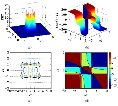
function in the 3-D space, the following scenario was considered: ω₃was chosen to be a set of fixed

values but ω1 andω2were permitted to vary freely. Numerical results show that when ω3is small, the

magnitude spectrum at the origin is large. Whenω₃becomes large, however, the magnitude spectrum

will be dominated by ωk =±ωk′and the peak at ωk =0becomes invisible. The graph of the output

frequency response function (33), corresponding to ω₃=0.5, is shown in Fig. 1, where the magnitude

and the phase spectrum, along with the relevant contour plots, are presented. Figure 1 clearly shows

that for the fixed valueω₃=0.5, the magnitude of the output frequency response function (33) has

seven peaks atω1=ω2=0,ω1=±1, and ω2 =±2. This fact is also reflected from the phase spectrum,

which varies smoothly from π to−π , passing the origin, whenω_k varies from negative values

(ωk <−ωk′) to positive values (ωk >ωk′) for k=1,2.

Fig. 1. The magnitude and phase spectra of the output frequency response function Φ(jω1, jω2,jω3)given by (33),

5. Conclusions

Based on the traditional integral transformations, the spatio-temporal transfer function (STTF) has

been introduced and applied to analyse, in the frequency domain, the inherent dynamics of a class of

spatio-temporal systems. The STTF, along with the relative frequency response function, can be used

to reveal the frequency properties of any given LTI spatio-temporal system, because every such

system possesses a unique STTF. By introducing the discrete time STTF, the analysis of dynamical

stability of the relevant systems become possible using existing theorems.

In this study, stability analysis of continuous STTF’s has not been investigated. How to analyse the

stability of a given LTI spatio-temporal system, directly using the associated continuous multivariable

STTF, is a topic for future study.

Acknowledgements

The authors gratefully acknowledge that this work was supported by the Engineering and Physical

Sciences Research Council (EPSRC), U.K.

References

B. D. O. Anderson and E. I. Jury, “Stability of multidimensional digital filters”, IEEE Transactions on

Circuits and Systems, CAS-21, pp.300-304, 1974.

W. F. Ames, Numerical Methods for Partial Differential Equations (3rd ed). Boston:Academic Press,

1992.

J. Bascompte and R.V. Sole (eds), Modelling Spatiotemporal Dynamics in Ecology. Berlin:

Springer-Verlag, 1998.

S. A. Billings and D. Coca, “Identification of coupled map lattice models of deterministic distributed

parameter systems”, International Journal of Systems Science, 33(8), pp.623-634, 2002.

S. A. Billings, L. Z. Guo and H. L. Wei, “Identification of coupled map lattice models for

spatio-temporal patterns using wavelets”, International Journal of Systems Science, 37(14),

pp.1021-1038, 2006.

Y. Bistritz, “Stability testing of dimensional discrete linear system polynomials by a

two-dimensional tabular form”, IEEE Transactions on Circuits and Systems I-Fundamental Theory and

Applications, 46, pp.666-676, 1999.

Y. Bistritz, “Testing stability of 2-D discrete systems by a set of real 1-D stability tests,” IEEE

Transactions on Circuits and Systems I-Regular Papers, 51, pp.1312-1320, 2004.

L. Chua, C. Ng, “Frequency-domain analysis of nonlinear systems: general theory, formulation of

transfer functions”, IEE Journal on Electronic Circuits and Systems, 3, pp.165-185, 1979.

patterns”, Physics Letters, A287, pp.65-73, 2001.

E. Curtin and S. Saba, “Stability and margin of stability tests for multidimensional filters”, IEEE

Transactions on Circuits and Systems I-Fundamental Theory and Applications, 46, pp. 806-809,

1999.

T. Czaran, Spatiotemporal Models of Population and Community Dynamics. London: Chapman &

Hall, 1998.

N. Damera-Venkata, M. Venkataraman, M. S. Hrishikesh, and P. S. Reddy, “A new transform for the

stabilization and stability testing of multidimensional recursive digital filters”, IEEE Transactions

on Circuits and Systems—II: Analog and Digital Signal Processing, 47, pp.965-968, 2000.

D. E. Dudgeon and R. M. Mersereau, Multidimensional Digital Signal Processing. Englewood Cliff,

NJ: Prentice-Hall, 1984.

D. G. Duffy, Transform Methods for Solving Partial Differential Equations (2nd ed). Boca Raton, Fla.:

Chapman & Hall/CRC, 2004.

G. Evans, J. Blackledge and P. Yardley, Analytic Methods for Partial Differential Equations. London:

Springer, 2000.

L.Z. Guo, S. A. Billings and H. L. Wei, “Estimation of spatial derivatives and identification of

continuous spatio-temporal dynamical systems”, International Journal of Control, 79 (9),

pp.1118-1135, 2006.

T. S. Huang, “Stability of two-dimensional recursive filters”, IEEE Transactions on Audio and

Electroacoustics, AU-20, pp.158-163, 1972.

B. Jahne, Spatio-Temporal Image Processing: Theory and Scientific Applications, Lecture Notes in

Computer Science, Vol. 751. Berlin: Springer-Verlag, 1993.

J. H. Justice and J. L. Shanks, “Stability criterion for n-dimensional digital filters”, IEEE Transactions

on Automatic Control, AC-18, pp.284-286, 1973.

K. Kaneko, Turbulence in coupled map lattices. Physics D, 18, pp.475-476, 1986.

J. K. Lubbock and V. S. Bansal, “Multidimensional Lapalce transforms for solution of nonlinear

equations”, Proc. Institution of Electrical Engineers, 116, pp. 2075-2082, 1969.

N. E. Mastorakis, “New necessary stability conditions for 2-D systems”, IEEE Transactions on

Circuits and Systems—I: Fundamental Theory and Applications, 47(7), pp. 1103-1105, 2000.

R. Parente, “Nonlinear differential equations and analytic system theory”, SIAM Journalon Applied

Mathematics, 18, pp. 41-66, 1970.

A. D. Polianin, Handbook of Linear Partial Differential Equations for Engineers and Scientists. Boca

Raton, Fla.: Chapman & Hall/CRC, 2002.

R. Rabenstein and L. Trautmann, “Multidimensional transfer function models”, IEEE Transactions on

Circuits and Systems I-Fundamental Theory and Applications, 49(6), pp.852-861, 2002.

R. P. Roesser, “Discrete state-space model for linear image-processing”, IEEE Transactions on

W. J. Rugh, Nonlinear System Theory—The Voterra/Wiener Approach. The John Hopkins University

Press, 1981.

J. L. Shanks, S. Treitel, and J. H. Justice, “Stability and synthesis of two-dimensional recursive filters”,

IEEE Transactions on Audio and Electroacoustics, AU-20, pp.115-128, 1972.

F.L. Silva, J.C. Príncipe, and L.B. Almeida (eds), Spatiotemporal Models in Biological and Artificial

Systems. Tokyo: IOS Press, 1997.

J. C. Strikwerda, Finite Difference Schemes and Partial Differential Equations. Pacific Grove,

California: Wadsworth & Brooks/Cole Advanced Books & Software, 1989.

M. G. Strintzis, “Test of stability of multidimensional filters”, IEEE Transactions on Circuits and

Systems, CAS-24, pp. 432-437, 1977.

H. Zhang and S. A. Billings, “Analysing nonlinear systems in the frequency domain—I: The transfer

Function”, Mechanical Systems and Signal Processing, 7, pp.531-550, 1993.

H. Zhang and S. A. Billings, “Analysing nonlinear systems in the frequency domain—II: The phase