Modelling Safety-Related Driving Behaviour - the Impact of Parameter Values

(1)

This is a repository copy of

Modelling Safety-Related Driving Behaviour - the Impact of

Parameter Values

.

White Rose Research Online URL for this paper:

http://eprints.whiterose.ac.uk/2487/

Article:

Bonsall, P.W., Liu, R. and Young, W. (2005) Modelling Safety-Related Driving Behaviour -

the Impact of Parameter Values. Transportation Research A, 39 (5). pp. 425-444.

https://doi.org/10.1016/j.tra.2005.02.002

[email protected] https://eprints.whiterose.ac.uk/ Reuse

See Attached

Takedown

If you consider content in White Rose Research Online to be in breach of UK law, please notify us by

(2)

Universities of Leeds, Sheffield and York

http://eprints.whiterose.ac.uk/

Institute of Transport Studies

University of Leeds

This is an uncorrected proof version of a paper originally published in

Transportation Research A. It has been peer reviewed, but does not include the

final publisher’s corrections.

White Rose Repository URL for this paper:

http://eprints.whiterose.ac.uk/2487

Published paper

Bonsall, P.W.; Liu, R.; Young W. (2005) Modelling Safety-Related Driving

Behaviour - the Impact of Parameter Values - Transportation Research. Part A:

Policy & Practice 39(5) pp425-444

(3)

UNCORRECTED

PROOF

2

Modelling safety-related driving behaviour—impact

3

of parameter values

4

Peter Bonsall

a

, Ronghui Liu

a,*

, William Young

b

5 a_{Institute for Transport Studies, University of Leeds, Leeds LS2 9JT, UK}

6 b

Department of Civil Engineering, MonashUniversity, Australia

Received 9 June 2004

9 Abstract

10 Traffic simulation models make assumptions about the safety-related behaviour of drivers. These

11 assumptions may or may not replicate the real behaviour of those drivers who adopt seemingly unsafe

12 behaviour, for example running red lights at signalised intersections or too closely following the vehicles

13 in front. Such behaviour results in the performance of the system that we observe but will often result in

14 conflicts and very occasionally in accidents. The question is whether these models should reflect safe

behav-15 iour or actual behaviour. Good design should seek to enhance safety, but is the safety of a design

neces-16 sarily enhanced by making unrealistically optimistic assumptions about the safety of drivers_Õbehaviour?

17 This paper explores the questions associated with the choice of values for safety-related parameters in

18 simulation models. The paper identifies the key parameters of traffic simulation models and notes that

sev-19 eral of them have been derived from theory or informed guesswork rather than observation of real

behav-20 iour and that, even where they are based on observations, these may have been conducted in circumstances

21 quite different to those which now apply. Tests with the micro-simulation model DRACULA demonstrate

22 the sensitivity of model predictions—and perhaps policy decisions—to the value of some of the key

param-23 eters. It is concluded that, in general, it is better to use values that are realistic-but-unsafe than values that

24 are safe-but-unrealistic. Although the use of realistic-but-unsafe parameter values could result in the

adop-25 tion of unsafe designs, this problem can be overcome by paying attention to the safety aspects of designs.

0965-8564/$ - see front matter _{2005 Published by Elsevier Ltd.}

doi:10.1016/j.tra.2005.02.002

*_{Corresponding author. Tel.: +44 113 3435338; fax: +44 113 3435334.}

E-mail address:[email protected](R. Liu).

www.elsevier.com/locate/tra

Transportation Research Part A xxx (2005) xxx–xxx

TRA 518 No. of Pages 21, DTD = 5.0.1

(4)

UNCORRECTED

PROOF

26 The possibility of using traffic simulation models to produce estimates of accident potential and the

diffi-27 culties involved in doing so are discussed.

28 _{2005 Published by Elsevier Ltd.}

29

30 1. Background

31 It is widely recognised that vehicles are sometimes, perhaps often, driven unsafely. Some drivers 32 are ignorant of such fundamentals as safe stopping distances and others willfully ignore them— 33 usually in order to get to their destination more quickly. Should models seek to replicate such 34 behaviour? On the one hand it might be held that models should be as accurate as possible 35 and that if unsafe behaviour occurs in real life it would be wrong to pretend otherwise. On the 36 other hand, it could be thought unethical to design a scheme using a tool which assumes unsafe 37 behaviour if this could lead to the adoption of designs which are known to be unsafe.Is it ‘‘right’’

38 in a detailed traffic simulation model to use parameter values which represent the actual behaviour of

39 drivers even though this behaviour might be unsafe,or would the use of unsafe parameters contribute

40 to the adoption of unsafe designs?and, to the extent that the answer to this question is ambiguous,

41 should ethical issues impinge on the selection of parameter values?

42 These were the questions which seem incapable of quick resolution and intriguing in their ram-43 ifications, and which therefore stimulated us to write this paper. We agreed that, in exploring the 44 issue, we should question where the parameters in well known traffic micro-simulation models 45 have come from and whether they represent real behaviour or some idealised safe behaviour. 46 We should investigate the sensitivity of model predictions to the value of key safety-related 47 parameters and should discuss the whole question of the representation of unsafe situations in 48 traffic micro-simulation models. Having done this, we should consider the consequences of using 49 safe-but-unrealistic and realistic-but-unsafe parameters and then attempt to come to a conclusion 50 on the question of the ethical, and potentially legal, issues involved in the choice of model param-51 eter values. This paper attempts to follow that agenda.

52 2. Safety-related parameters in traffic simulation models

53 The progress of individual vehicles in a detailed traffic simulation model is the result of applying 54 rules and formulae to determine aspects such as:

55 •_{speeds in free-flowing traffic;}

56 •_{headways between vehicles;}

57 •_{acceleration and deceleration profiles;}

58 •_{interaction between priority and non-priority vehicles;}

59 •_{overtaking and lane-changing behaviour; and}

60 •_{adherence to traffic regulations—notably compliance with traffic signals and adherence to}

6162₆₃ speed limits but also to regulations on the use of bus lanes, one-way streets, banned-turns, etc.

2 P. Bonsall et al. / Transportation ResearchPart A xxx (2005) xxx–xxx

(5)

UNCORRECTED

PROOF

64 All of which are obviously related to safety. In fact, asYoung et al. (1989) point out, most of 65 the parameters used in micro-simulation models have implications for safety—even a parameter 66 as seemingly neutral as the simulation interval will have an impact on safety if, as is commonly the 67 case, it effectively defines the drivers_Õreaction time.

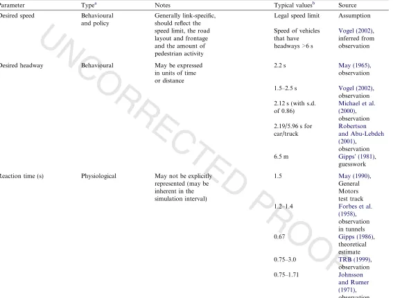
68 Most of the behaviours listed above are determined in traffic simulation models via sub-models 69 representing car-following, gap-acceptance and lane-changing behaviour. These models are, in 70 turn, dependent on parameters which are deemed to encapsulate the relevant aspects of driver 71 behaviour. These models, the associated parameters and the values typically adopted for them 72 are described in the following sub-sections and summarised in Table 1.

73 2.1. Car-following models

74 Car-following models represent the longitudinal interaction among vehicles in a single stream 75 of traffic. The speed of the following vehicle is assumed to respond to stimulus from the vehicle or 76 vehicles in front. The stimulus is usually represented in terms of distance and speed differences. 77 One of the widely used car following model is that proposed by Gipps (1981) which combines 78 a free-flow driving model with a stopping-distance based car-following behaviour model. This 79 model, or variations on it, has been implemented in micro-simulation software packages such 80 as AIMSUN (Barcelo et al., 1995), SISTM (Wilson, 2001), and DRACULA (Liu, 2003). 81 Some authors reserve the termÔcar-followingÕexclusively for the preceding/following situation 82 while others extend it to cover anything related to the longitudinal progress of vehicles (thus 83 including the determination of free-flow speeds, acceleration and deceleration profiles and re-84 sponse to traffic signals). We need not concern ourselves here with such distinctions, nor with 85 the variety of forms that the car-following models can take; our immediate concern is solely with 86 the parameters required to determine the longitudinal progress of vehicles.

87 Taking the broadest definition of the car-following model, the main parameters used in the 88 models are:

89 2.1.1. Desired speed

90 Desired speeds of the drivers are generally modelled as input parameters and are often directly 91 made equal to the free-flow speeds on the link or road. The later may vary according to the char-92 acter of the road. For example, a dual-carriage road and a wider road may lead to higher free-flow 93 speeds than residential streets. City-centre streets where there are lots of pedestrians and pedes-94 trian crossings will force the free-flow speeds down, as would excessive curvature or gradient. 95 Speed limits are used as a proxy for free-flow speeds—a practice with interesting implications 96 to which we will return in a later section of the paper.

97 2.1.2. Desired headway

98 Car following algorithms generally assume a minimum safe headway which a following vehicle 99 wishes to keep. This may be represented as either a time or a distance headway. When the follow-100 ing and the lead vehicle driver are at the same speed, the time headway represents the time avail-101 able to the driver of the following vehicle to reach the same level of deceleration as the lead vehicle 102 in case it brakes. This available time is independent of speed. The Gipps model uses a 1–2 s time 103 headway.

P. Bonsall et al. / Transportation ResearchPart A xxx (2005) xxx–xxx 3

(6)

UNCORRECTED

[image:6.743.87.654.69.499.2]

PROOF

Table 1

Safety-related parameters commonly included in traffic simulation models

Parameter Typea Notes Typical valuesb Source

Desired speed Behavioural and policy

Generally link-specific, should reflect the speed limit, the road layout and frontage and the amount of pedestrian activity

Legal speed limit Assumption

Speed of vehicles that have headways >6 s

Vogel (2002), inferred from observation

Desired headway Behavioural May be expressed in units of time or distance

2.2 s May (1965), observation

1.5–2.5 s Vogel (2002), observation 2.12 s (with s.d.

of 0.86)

Michael et al. (2000), observation 2.19/5.96 s for

car/truck

Robertson and Abu-Lebdeh (2001),

observation 6.5 m GippsÕ(1981),

guesswork

Reaction time (s) Physiological May not be explicitly represented (may be inherent in the simulation interval)

1.5 May (1990),

General Motors test track 1.2–1.4 Forbes et al.

(1958), observation in tunnels 0.67 Gipps (1986),

theoretical estimate 0.75–3.0 TRB (1999),

(7)

UNCORRECTED

PROOF

0.85–1.6 for young drivers

Olson et al. (1984), observation 0.57–1.37 for

older drivers

Olson et al. (1984), observation 1.5–3.0 Neuman (1989), observation 2.74 McGee (1989), observation Rate of

acceleration (m/s2₎

Behavioural (constrained by vehicle performance)

May distinguish between normal rate of acceleration and maximum rate of acceleration, may differ depending on vehicle type

For cars:

1.5–3.6 max acceleration

ITE (1982), observations? 0.9–1.5 normal

acceleration

Gipps (1981), theoretical estimate For buses: 1.2–1.6 Firstbus (private communication)

Rate of

deceleration (m/s2₎

Behavioural (constrained by vehicle performance)

My distinguish between normal deceleration and emergency braking, may differ by vehicle type

1.5–2.4 emergency ITE (1982), observations? 0.9–1.5 normal ITE (1982),

observations?

3.0 Gipps (1981),

theoretical estimate

Critical gap (s) Behavioural From the back of one vehicle in the target stream to the front of the following vehicle in that stream

3.5 Gipps (1981),

theoretical estimate

4.75 Kimber et al.

(8)

UNCORRECTED

PROOF

Stimulus required to induce use of the reduced gap (s)

Behavioural Time spent waiting for acceptable gap number of rejected gaps

120 Mahmassani

and Sheffi (1981), guesswork

Minimum gap (s) Behavioural 1.0 Guesswork

Willingness to create gaps to assist other vehicles

to change lanes

Behavioural May be expressed as the percentage of the priority traffic stream who stop accelerating or even start decelerating once they ‘‘see’’ there is minor flow traffic waiting to merge or cross. May vary depending on what type of the other vehicles are.

20% for other cars Guesswork

70% for buses

Rules for mandatory lane change

Behavioural and policy May simply reflect traffic regulations but may vary depending on enforcement policy

Published regulations n.a.

How far ahead the drivers anticipate the need to change lanes

Behavioural and policy The behavioural element may be constrained by sight lines, etc.

1 to 2 links, or 500 m Liu (2003), Nsour and Santiago (1994), guesswork

Minimum acceptable gap when changing lanes

Behavioural As in gap-acceptance model As in gap-acceptance model

As in gap-acceptance model

Variation in the gap depending on the urgency of the desire to change lanes

Behavioural May depend on size of time advantage or distance remaining before mandatory change must be completed

50–100 m or 5–10 s Guesswork

(9)

UNCORRECTED

PROOF

Willingness to create gaps to assist other vehicles to change lanes

Behavioural May be expressed as the percentage of the traffic in the target lane who stop accelerating/start decelerating once they ‘‘see’’ a vehicle attempting to enter the lane

20% for other cars Guesswork

70% for buses

Level of compliance Behavioural and policy May differ for different types of regulation

50–100% Some observations e.g.Gipps (1986) for lane changing, and

Should vary depending on enforcement policy

Liu and Tate (2004)for speed compliance

Distribution of aggressiveness

Behavioural Sometimes used to control the proportion of drivers in each of several preset categories, each category being characterised by different values for each of the aggression-related parameters described above. Used to make model predictions fit observed indicators of the operational

performance of the system (e.g. speed, throughput)

n.a. n.a.

a _{Note that, when modelling the performance of advanced driver-assistance devices or of a full automated highway system, several of these}

parameters would become functions of the system specification and thus, effectively, they become policy variables. For example, in work to test the impact of in-vehicle speed control devices on the operational performance of a network, Liu and Tate (2000) modified parameters in DRACULA to make speed limit compliance vary as a function of the assumed penetration of speed control devices in the vehicle fleet.

b_{Note that most models use a distribution of values in preference to a single value.}

P.

Bonsall

et

al.

/

Transportation

ResearchPart

A

xxx

(2005)

xxx–xxx

7

TRA

518

No.

of

Pages

21,

DTD

=

5.0.1

10

March

2005

Disk

Used

ARTICLE

IN

(10)

UNCORRECTED

PROOF

104 2.1.3. Reaction time

105 Reaction time is a key dimension in both car-following and lane-changing models. It represents 106 the driverÕs ability to react to situations and make particularly decisions. Gipps used a 2/3 s reac-107 tion time for all drivers, whilst DRACULA samples from a range between 0.8–2.0 s for individual 108 drivers.

109 2.1.4. Normal and maximum acceleration

110 Drivers may apply a smaller acceleration in a more relaxed following situation, whilst they may 111 apply the full acceleration power of their engine when trying to overtake or pass through a green 112 light. A normal acceleration rate of 1.2 m/s2, and a maximum acceleration of 1.6 m/s2for cars has 113 been assumed by Gipps.

114 2.1.5. Normal and maximum deceleration

115 Drivers may apply a gentler deceleration when approaching a known obstacle or an obstacle 116 visible a long way upstream, such as approaching a traffic light or a slower moving vehicle in 117 front. A harsher deceleration may be applied for emergency breaking, such as in response to a 118 sudden deceleration of the vehicle in front or to a sudden lane-changing from adjacent traffic. 119 A normal deceleration of 2.5 m/s2 and maximum deceleration of 5.0 m/s2 are the default values 120 adopted in DRACULA.

121 2.2. Gap-acceptance models

122 Gap-acceptance models deal with process by which a driver finds an acceptable gap in a traffic 123 stream when (s)he wants to cross or merge into that stream. They are fundamental in representing 124 conflicts between high and low priority flows and in determining how a vehicle from a low priority 125 flow will cross or merge into a higher priority flow. The models are used to deal with aspects such 126 as overtaking which involves use of the opposing carriageway (how much of a gap in the opposing

127 flow is required?), lane-changing (how much of a gap or gaps in the traffic using the intended lane?),

128 and uncontrolled pedestrian movements (how much of a gap in the traffic flow will a pedestrian

re-129 quire before attempting to cross a carriageway?).

130 Gaps are usually represented in time (s). The key parameters for gap-acceptance models 131 include:

132 2.2.1. Critical gap

133 A driver or pedestrian will accept a gap in the traffic stream to contemplate his intended 134 manoeuvre if the gap is longer than the critical gap (Hewitt, 1983). The critical gap will clearly 135 differ between drivers and it is therefore modelled in DRACULA and some other models as a ran-136 dom variable drawn from an assumed probability density distribution of critical gaps in the 137 population.

138 2.2.2. Gap-reduction and minimum gap

139 Some gap-acceptance models use a fixed value for each driver, others allow critical gaps to be 140 situation-dependent in order o reflect the phenomenon of impatient drivers for whom the critical 141 gap decreases with each passing gap (Kimber, 1989). This gap-reduction behaviour can be

recog-8 P. Bonsall et al. / Transportation ResearchPart A xxx (2005) xxx–xxx

(11)

UNCORRECTED

PROOF

142 nised by observing drivers who reject a gap which is longer than the one eventually accepted. The 143 stimulus required to induce the decrease of critical gap has been modelled as the number of pass-144 ing gaps (e.g.Mahmassani and Sheffi, 1981) and, in DRACULA, as the time spent in searching 145 for acceptable gap. Clearly, the critical gap can not decrease infinitely, hence a minimum gap is 146 often used in the models to set a lower boundary to the formulation.

147 2.2.3. A ‘‘gap-creation’’ situation

148 Some gap-acceptance models allow for the fact that drivers in the priority flow may take pity on 149 drivers waiting for a gap and may deliberately slow down in order to create a gap. This is repre-150 sented in DRACULA via a parameter to indicate the percentage of traffic having awillingness to

151 create gaps.

152 2.3. Lane-changing models

153 Lane-changing models consider the individual driverÕs intention and ability to change lanes. An

154 intentionto change lanes will reflect the advantage to be gained (e.g. an increase in speed or an

155 avoidance of delay) or the need to do so (e.g. in order to comply with a traffic regulation, to avoid 156 an incident in the current lane, or to prepare for a turning movement). The intention to make a 157 lane-change may be triggered when the time advantage to be gained by changing lanes exceeds 158 some critical value. Some models may allow drivers to anticipate the need for a change of lane, 159 in which case a parameter will be required to determinehow far ahead the drivers anticipate.

160 Theabilityto change lanes will be a function of the lane space available and the relative speeds

161 and locations of surrounding vehicles and is generally modelled in a way which is analogous to a 162 gap-acceptance model. The parameters controlling this model will thus include the minimum

163 acceptable gap in the target lane, together, perhaps, with parameters which allow for variation

164 in the gap depending on the urgency of the desire to change lanes (see Taylor et al., 2000), and

165 the willingness to create gapsby kind-hearted drivers in the target lane.

166 The driverÕs intention to change lanes is a complex decision-making behaviour, involving an-167 swer questions such as:is it possible to change lane? Is it necessary to change lane? and is it desirable

168 to change?The lane-changing models need first of all to identify the reasons for such intention.

169 The following are a list of but few: bus stopping at bus stops; avoiding an incident (parked vehicle, 170 road works, accidents); making junction turning movements; and overtaking a slower moving 171 vehicle.

172 Perhaps the most complicated part of a lane-changing model is its formulation of a driverÕs 173 lane-changing intention as decision-making tree. It appears that there is no universally accepted 174 structure for this process; each model or package has a unique list of lane-changing reasons a un-175 ique structure for the decision-making process.

176 Once a lane-changing intention is triggered, a gap-acceptance model is used to find the gaps in 177 the target lane which are acceptable to the driver wishing to change lanes. The parameters con-178 sidered here are front gap and rear gap (lag) in the traffic stream of the target lane, and the critical 179 gap acceptable to the driver. The parameters in the gap-acceptance models for lane-changing sit-180 uation are similar to those in the general gap-acceptance models described above.

(12)

UNCORRECTED

PROOF

181 2.4. Adherence to regulations

182 This factor is rarely introduced into models. Adherence to traffic regulations may be modelled 183 using assumedlevels of compliance—these may differ for different types of regulation and should, 184 ideally be treated as policy variables reflecting different levels of enforcement.

185 2.5. Representations of parameter values

186 Most models use a distribution of values, rather than a single value, for their key behavioural 187 parameters. It should also be noted that, although some models use the same parameter value, or 188 distribution of values, for all vehicles and drivers, others allow different values or distributions for 189 different classes of vehicle and for differentÔtypesÕof driver. For example, the PARAMICS (Laird 190 et al., 1999) and CORSIM (Rathi and Santiago, 1990) models recognise various categories of dri-191 ver according to theÔaggressivenessÕof their driving style (the more aggressive drivers accept smal-192 ler gaps, accelerate and decelerate more rapidly, and so forth). The proportion of people in each 193 preset_Ôaggressiveness_Õ category is not based on any real data but is a variable which can be ad-194 justed as part of the process of getting the simulation model to reproduce aggregate statistics such 195 as average speeds or flow throughput. The process of model fitting is of course crucial to the use of 196 the model but, as we will see later in this paper, it can be argued that problems are likely to occur 197 if this is done simply by adjusting the proportion of drivers in each of the preset aggressiveness 198 categories. The DRACULA model (Liu et al., 1995) allows the user to specify the distribution 199 of values for each parameter—an approach which overcomes the problem of using preset aggres-200 siveness categories but which obviously requires more data.

201 2.6. Summary of data sources

202 Table 1 lists the parameters identified above, indicating commonly adopted values and the 203 sources of these values. The second column of the table distinguishes between purely behavioural 204 parameters, those which represent behaviour which is constrained by vehicle performance, those 205 which reflect policy and those (of which reaction time is the only example) which are in some sense 206 fundamental. It can be argued that each of these types of parameter has a different role in the 207 model and that different rules should apply in selecting values for them.

208 The fourth column ofTable 1presents typical values for the parameters but it is clear that, for 209 some parameters, quite different values are adopted in different models—although it should be 210 noted that, due to differences in the models, not all the values are strictly comparable.

211 It is apparent from the fifth column ofTable 1that the values of several of the key parameters 212 are based on speculation or theory rather than on actual observations. Even those which are based 213 on observations are often reliant on data for a limited range of vehicle types and, in some cases, on 214 data collected decades ago in particular driving conditions and their applicability to 21st century 215 driving conditions, sometimes on different continents, may be questioned.

(13)

UNCORRECTED

PROOF

216 3. The impact of unsafe driving on system performance

217 3.1. Acceptance of risk—how drivers really drive

218 Before examining the implications for model predictions it is worth considering the impacts 219 that unsafe driving has for system performance. Section 2 has listed a number of key parameters 220 in simulation models. This section explores some of them in a little more detail and, introduces the 221 concept of risk. Risk represents the probability of an accident occurring. Drivers accept risk when 222 they drive a car and behave in the light of their own perception of the size of the risk and of their 223 attitude to it.

224 It is not difficult to think of situations in which a proportion of drivers, perhaps the majority, 225 drive in a way that is not commensurate with maximum safety. These obviously include:

226 • _{adoption of inadequate headways in fast moving traffic (below the calculated} _Ô_{safe stopping}

227 distance_Õ),

228 • _{speeding (in excess of the legal limit or in spite of local circumstances),}

229 • _{excessive reliance on the vehicle}_Õ_{s brakes (even in adverse weather conditions),}

230 • _{nearside overtaking (where illegal and therefore unexpected by other drivers),}

231 • _{reckless overtaking (e.g. where sight-lines are inadequate),}

232 • _{passing traffic signals at orange (or even red).}

233

234 We will consider some of these in a little more detail and, in doing so, will recall that most driv-235 ers have no precise idea of how safe or dangerous a manoeuvre might be but that they make 236 assumptions based on assumptions about their reaction times and those of other drivers, and 237 about the performance of their vehicles. A driver_Õs reaction time is a key determinant of the degree 238 of safety with which he can complete a given manoeuvre or maintain a given headway. In reality, 239 many drivers overestimate the speed of their reactions and, by driving accordingly, they are con-240 tributing to a marginal increase in system performance but also to the likelihood of an incident 241 which, were it to occur, would have severe consequences for system performance as well as for 242 life and limb.

243 3.1.1. Safe headways

244 Simplifying somewhat, the reaction time assumed by UK highway designers in the determina-245 tion of stopping sight distance is 2 s (DOT, 1993). If all the vehicles were travelling at the same 246 speed then a vehicle that immediately stops would require the following vehicle to be travelling 247 at a headway of 2 s. This separation headway would result in traffic flows of 1800 vehicles per lane 248 per hour. However, research has shown that freeway traffic moves at much lower headways and 249 thereby achieves much higher flows per lane.

250 Research by Oates (1999) suggested that almost 50% of drivers on congested stretches of the 251 M62 motorway were driving with headways at or below 2 s and that almost 25% were driving with 252 headways at or below 1 s. This clearly indicates that drivers are driving unsafely. Simple calcula-253 tion indicates that, in smooth conditions and constant speed, the flow achievable with a 0.5 s 254 headway would be about four times that achievable with a 2 s headway. However, the adoption 255 of 0.5 s headways would clearly assume unsafe behaviour since no vehicle could stop if the vehicle P. Bonsall et al. / Transportation ResearchPart A xxx (2005) xxx–xxx 11

(14)

UNCORRECTED

PROOF

256 in front suddenly stopped at this speed, hence causing incidents. Given that incidents are likely to 257 be more frequent at low headways and that, until the debris is removed and the shockwaves have 258 dissipated, incidents have a dramatic effect on network performance. Maximum network perfor-259 mance is probably achieved at average headways of around 1.5 s.

260 3.1.2. Gap acceptance

261 A driverÕs gap-acceptance behaviour is a function of his or her perception of risk and reward. 262 This perception can change—for example acceptance of risk tends to increase if a driver has al-263 ready been waiting a long time (Taylor et al., 2000). In real life, the choice of short gaps will some-264 times, all be it rarely, result in an accident and consequential delay to traffic but more usually it 265 will help to keep the network moving.

266 3.1.3. Stopping at red lights

267 Traffic signals are used as safety devices and to manage the flow of traffic by temporal separa-268 tion of conflicting movements. The rule is that drivers should stop at traffic signals when the lights 269 are red. In practice, of course, many drivers do go through red lights and this is pragmatically 270 recognised by the inclusion of all-red phases even though incorporation of dead time reduces 271 the performance of the system. In fact the potential deterioration in performance is marginally 272 reduced because some drivers do disobey the rules; Pretty (1974) found that traffic signals im-273 proved capacity at an intersection previously under police control only because drivers used 274 the amber and all-red periods.

275 3.1.4. Adherence to speed limits

276 Roads are generally designed for a speed which is exceeded by no more than 15% of the traffic. 277 In his development of relationships between speeds and the geometric characteristics of rural 278 roads,McLean (1978)concluded that about 15% of drivers were likely to exceed the speed limit 279 and that optimal design should recognise this fact. It is commonly observed that free-flow speeds 280 are often well in excess of the speed limit and that, in the absence of congestion, such speeds ap-281 pear to be able to be maintained almost indefinitely.

282 3.2. The impacts of unsafe driving on network performance—in reality and in models

283 Similar arguments can be made in respect of each of the unsafe-driving cases mentioned earlier. 284 Unsafe driving will generally lead to enhanced system performance but when, as is inevitable, 285 there is an incident, the results can be catastrophic not only for life, limb and property, but also 286 in terms of disruption to the smooth flow of traffic. On balance, however, provided that incidents 287 remain relatively rare events, it is reasonable to conclude that if everyone were to drive in strict

288 accord withguidelines and regulations,the effective capacity of the network would be reduced below

289 the levels currently observed.

290 However, most simulation models do not allow accidents to occur and so ignore the question of 291 risk and of the consequences that an accident might have for network performance. By ignoring 292 the possibility of these rare events, traffic simulation models are representing only one side of the 293 safety/efficiency equation; the half that sees only benefit from driversÕacceptance of higher risks.

(15)

UNCORRECTED

PROOF

294 They have no mechanism for reflecting the advantage of safety measures such as stricter enforce-295 ment of speed limits or the incorporation of all-red phases at traffic lights.

296 If a simulation model were to assume that all drivers adopted headways which were safe, this 297 would, given a realistic distribution of reaction times, require the assumption of longer headways 298 than are observed in practice and this would result in an underestimate of achievable traffic flows 299 and hence in incorrect estimates of the performance of the traffic system. Similarly, if traffic sim-300 ulation models were to allow that not all drivers stop at red lights this would result in an under-301 estimate of the achievable traffic flow.

302 As noted in a previous section, simulation models commonly assume that drivers_Õdesired speed 303 is the free-flow speed and that this may be proxied by the speed limit. This assumption not only 304 raises the curious concept of a limit which no one wishes to exceed (in which case why is it 305 needed?) but, more seriously in the current context, implies that all vehicles will travel at or below 306 the speed limit irrespective of the lightness of the flow. This assumption must result in an under-307 estimate of the performance of the traffic system.

308 4. Simulation tests

309 In order to illustrate the general argument made above, the DRACULA model was used to ex-310 plore the impact that changes in key behavioural parameters might have on various model esti-311 mates of system performance. The results reported here relate primarily to the total travel time 312 in the test network since this is the indicator of system performance most widely used to inform 313 investment decisions.

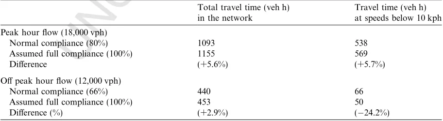
314 The first test was designed to show the effect of unrealistically assuming full compliance with 315 speed limits. The test was based on an urban network in east Leeds covering an area of 3 km 316 by 10 km. The results, shown in Table 2, relate only to traffic on the roads subject to a 30 mph 317 (50 kph) speed limit.

[image:15.544.42.498.536.661.2]

318 It is clear that, if we assume full compliance with the speed limit, the total travel time in the 319 network would increase. Given that the observed level of compliance is lower in the off-peak per-320 iod, one might have expected that the effect of assuming 100% compliance would be more marked 321 in the off-peak. In fact this is not the case. The off-peak effect seems to be reduced because of a

Table 2

Predictions of the effect of different levels of speed limit compliance

Total travel time (veh h) in the network

Travel time (veh h) at speeds below 10 kph Peak hour flow (18,000 vph)

Normal compliance (80%) 1093 538

Assumed full compliance (100%) 1155 569

Difference (+5.6%) (+5.7%)

Off peak hour flow (12,000 vph)

Normal compliance (66%) 440 66

Assumed full compliance (100%) 453 50

Difference (%) (+2.9%) ( 24.2%)

(16)

UNCORRECTED

PROOF

322 marked reduction in congestion (as indicated by total travel times at speed below 10 kph) during 323 this period. We speculate that this is because, in the absence of the fast vehicles, there is less to 324 interfere with the smooth flow of traffic during low flow conditions than there is during the peak 325 (Liu and Tate, 2004).

326 The results of this test demonstrate how a change in the assumed compliance with speed limits 327 can affect the overall performance of the system and that this effect differs according to the time of 328 day in ways which might not have been predicted in advance.

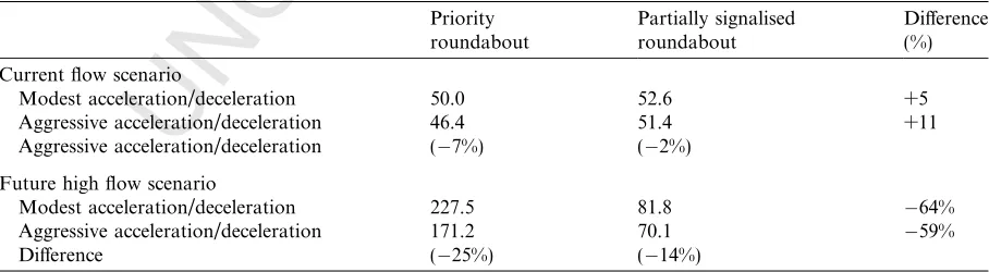
[image:16.544.46.504.383.523.2]

329 The second set of tests was designed to show how assumptions about the distribution of one 330 aspect of aggressive driving (in this case the normal and maximum rates of acceleration and decel-331 eration) can affect the predicted performance of a scheme. The tests relate to the introduction of 332 partial signalisation at a roundabout just off the M25 near Heathrow Terminal 5. The mean values 333 of the acceleration/deceleration distributions used in the tests are shown inTable 3(note that traf-334 fic at the site is 10% HGV and 90% car). The tests relate to two flow level scenarios; a current flow 335 and a future flow at twice the current level—as can be expected when the new Terminal opens. 336 The results of the tests are shown inTable 4. As might be expected, the effect of the signalisation 337 scheme is very dependent on the assumed level of flow; at current flow levels the signalisation 338 would lead to an increase in journey times whereas, at future high levels, it would lead to a very 339 marked reduction in journey times. More interestingly, in the light of the theme of the current 340 paper, it is clear that the assumed level of acceleration/deceleration affects the predicted impact

Table 3

Mean acceleration and deceleration rates used in the roundabout signalisation tests Default acceleration and

deceleration

More aggressive acceleration and deceleration

Car HGV Car HGV

Normal acceleration (m/s2₎ _1.5 _1.2 _2.5 ₂

Max acceleration (m/s2) 2 1.6 2.5 2

Normal deceleration (m/s2) 2 1.5 2.5 2

Max deceleration (m/s2₎ ₅ _2.5 ₅ _3.5

Table 4

DRACULA predictions of the effect of roundabout signalisation, measured in vehicle hours in the local network Priority

roundabout

Partially signalised roundabout

Difference (%) Current flow scenario

Modest acceleration/deceleration 50.0 52.6 +5 Aggressive acceleration/deceleration 46.4 51.4 +11 Aggressive acceleration/deceleration ( 7%) ( 2%)

Future high flow scenario

Modest acceleration/deceleration 227.5 81.8 64% Aggressive acceleration/deceleration 171.2 70.1 59%

Difference ( 25%) ( 14%)

[image:16.544.48.502.535.660.2]

(17)

UNCORRECTED

PROOF

341 of the signalisation scheme. If a more aggressive level of acceleration/deceleration is assumed, 342 journey times are much reduced—particularly while the roundabout is operating under normal 343 priorities and under the high flow scenario.

344 The net result is that the assumption of more aggressive acceleration/deceleration causes a dou-345 bling of the dis-benefit associated with signalisation under current flow conditions but causes a 346 reduction in the large benefit predicted under high flow conditions. It is clear that the assumptions 347 about levels of acceleration and deceleration can profoundly affect the prediction of scheme ben-348 efits and that this effect differs according to the flow level.

349 5. Discussion

350 5.1. Implications of choice of parameter values on safety

351 The previous sections have highlighted some of the key safety-related parameters in simulation 352 models and provided examples to illustrate the choice of parameter values on system perfor-353 mance. Clearly, the value of the parameters will affect the model predictions, but what are the 354 implications of this for design, for investment decisions, and for the behaviour of travellers? 355 We will consider this question separately for the different types of parameter identified inTable 1. 356 Errors inparameters reflecting fundamentals of human physiology or of the performance of

vehi-357 cles or system components could have serious implications for the design of system components

358 such as sight lines or inter-greens. For example; an overoptimistic assumption about driversÕ reac-359 tion times or vehicles_Õbraking performance will lead to overestimation of the operational perfor-360 mance (defined in terms of flows and journey times) and of the safety of the system. Pessimistic 361 assumptions will lead to similar underestimations. Although both might lead to sub-optimal 362 investment decisions, it can be argued that the results of an overestimation of the operational per-363 formance and safety of a system are potentially more severe than those of an underestimation. 364 Overestimation of operational performance or safety may lead to the adoption of unsafe or inef-365 ficient designs, underestimation of performance or safety may lead to over specification of the de-366 sign and, as a consequence of this, perhaps to fewer schemes being built. It seems reasonable to 367 conclude that the analyst should therefore err on the side of underestimating the capabilities of 368 drivers, their vehicles and other system components.

369 For parameters reflecting policy or behaviourthe situation is much more complex because the

370 consequences of using the wrong parameter value will depend on the way that the model is being 371 used. This complexity results from the fact that a given error in the parameter value will affect the 372 predictions of operational performance in the opposite direction. For example, if the assumed 373 adherence to speed limits is too low the model will over estimate the operational performance 374 of the system whereas if the assumed adherence to speed limits is too high the model will under-375 estimate the operational performance of the system. As will be seen, the consequences of this will 376 be quite different depending on the way the model is being used.

377 We begin by considering the situation where the model is being used to identify schemes which 378 meet predefined operational performance criteria. The use of safe-but-unrealistic parameter values 379 in such circumstances will result in the rejection of schemes which would have met the criteria had 380 more realistic values been used. This in turn would tend to lead to the adoption of schemes whose P. Bonsall et al. / Transportation ResearchPart A xxx (2005) xxx–xxx 15

(18)

UNCORRECTED

PROOF

381 capacities, and costs, are greater than necessary. Not only would this represent misuse of re-382 sources but the oversupply of capacity might lead to the induction of additional traffic. The 383 use of realistic-but-unsafe parameter values would produce no such problems. However, if the 384 candidate schemes are not subject to safety audit and if no estimate of the safety of each scheme 385 is being produced by the model, it is clearly possible that unsafe designs would be adopted—we 386 return to the question of how traffic simulation models might produce indicators of safety in a 387 later section of this paper.

388 We now consider the situation where the model is being used as part of an evaluation of alter-389 native schemes, including the do minimum, in order to identify the one which represents the best 390 value for money. The process will, by definition, include an assessment of the safety consequences 391 of each scheme as well as of its operational performance (although, in the absence of safety indi-392 cators from the traffic simulation model, the safety aspects may not be dealt with consistently— 393 again, we will return to this issue in a later section of this paper). There will be a general tendency 394 for unrealisticallyÔsafeÕparameter values to result in an underestimate of the operational perfor-395 mance of the scheme but to provide an over estimate of its safety. The use of unrealistically unsafe 396 parameter values will similarly tend to result in over estimation of the operational performance of 397 the scheme but underestimation of its safety. Either case would lead to incorrect assessment of 398 scheme worth and it would clearly be better to use realistic values for all parameters.

399 It should be noted, in passing, that, in order to avoid bias in the appraisal process, all parameter 400 values should be equally realistic. For example if the parameter value for, adherence to traffic sig-401 nals, were more unrealisticallyÔsafeÕthan any other parameter value, the model would underesti-402 mate the operational performance of (and overestimate the safety of) a scheme which involved a 403 major programme of signalisation. Conversely, an overly safe assumption about gap acceptance 404 would deflate the safety improvement (and inflate the operational improvement) to be expected 405 from signalisation of a priority intersection. The consequences of these errors would depend on 406 the relative weights given to the operational and safety aspects in the appraisal, but it would cer-407 tainly bias the outcome. The use of realistic-but-unsafe parameter values would not distort the 408 appraisal process provided that full account is being taken of the safety indications of each design. 409 If proper account isnotbeing taken of safety indications it is possible that the use of realistic-410 but-unsafe parameter values could promote the adoption of unsafe design elements. For example, 411 a model which allows unsafe overtaking would reflect the operational advantage to be gained by 412 this activity and would therefore tend to favour schemes which give most opportunity for it to 413 occur. Other things being equal, a scheme with a single carriageway comprising two lanes will 414 therefore operationally outperform one with a dual carriageway comprising one lane in each 415 direction. The implication is that, by allowing the model to represent unsafe behaviour, we would 416 be increasing the probability its occurrence.

417 It is worth noting that any error in the value ofparameters which are supposed to represent policy

418 variableswill mean that the system under test has been incorrectly specified; quite simply the model

419 predictions will not relate to the system of interest. As discussed above, the significance of this miss-420 specification will depend on the nature of the error and on the way that the model is being used. 421 Quite clearly, a fundamental contributor to the problems noted above is the concentration on 422 indicators of operational performance and the failure to consider indicators of safety. But this 423 myopia may be difficult to avoid if the model does not produce any indicators of safety. It is 424 to this issue which we now turn.

(19)

UNCORRECTED

PROOF

425 5.2. ModellersÕliability

426 The preceding discussion has introduced the question of accuracy versus reality. Models are 427 used in the design of elements of the traffic system. If the design of these elements involved 428 assumptions of unsafe behaviour what is the legal liability of the model developer should an acci-429 dent occur? The design may result in a more efficient traffic movement in terms of travel time, 430 operating cost and environmental impact. However it may require drivers to take unnecessary 431 risks. If a driver takes this risk and an accident occurs the design may be unsafe and the modeller 432 developing the simulation may be seen as liable for the development of an unsafe design.

433 5.3. Accuracy and stability of existing simulation models

434 Existing simulation models are built with a set of assumptions. Could these models realistically 435 predict unsafe behaviour, given appropriate parameter values and the delay, which would occur 436 when an incident takes place? It may be necessary to develop a new set of models with more com-437 plex representation of behaviour.

438 The introduction of unsafe behaviour into simulation models could result in the decrease in the 439 stability of models. This may have considerable implications for ‘‘convergence’’ (or number of 440 simulation runs required) if allowance for random aspects of safety are introduced. The use of 441 the models may be made less attractive because of the need for longer run times.

442 5.4. Potential indicators of safety

443 It is quite possible to imagine a traffic simulation model being modified in order to predict the 444 occurrence of crashes. Existing sub-models could be enhanced to allow for a wider distribution of 445 driving styles, vehicle characteristics, infrastructure and weather conditions and, when a critical 446 set of conditions came together, a crash could be predicted. The occurrence of a crash could then 447 be allowed to create an obstacle which would interrupt the traffic flow, cause congestion, perhaps 448 inducing secondary crashes. . . and so on—a prospect which might well appeal to the creative

449 imagination of the modeller!

450 However, since crashes are rare events, little practical use could be made of predictions of their 451 occurrence until, in some future time the computing power allows thousands of days to be sim-452 ulated in a few minutes, the binary occurrence of crashes could be replaced by a probability. 453 In the meantime, allowing a traffic simulation model to predict crashes would bring with it the 454 inconvenience of increased instability in the prediction; the occurrence or non-occurrence of an 455 incident would so dominate the predicted operational performance of the scheme that it would 456 become necessary to increase the number of runs massively. For the foreseeable future it would 457 thus be more useful to predict conflicts or near-misses rather than actual crashes.

458 This might be done by making use of the concept of the_Ôtime-to-collision_Õ(TTC) between two 459 vehicles (or between a vehicle and a stationary object). TTC is defined as ‘‘the time for two vehi-460 cles to collide if they continue at their present speed and path’’ (Sayed et al., 1994). The value of 461 TTC is infinite if the vehicles are not on a collision course; but if the vehicles are on collision 462 course, the value of TTC is finite and decreases with time unless avoiding action is taken (Hoffman

(20)

UNCORRECTED

PROOF

463 and Mortimer, 1996). By logging the occurrence of all TTCs below a critical threshold, an indi-464 cator of near-misses could be produced.

465 An alternative approach, whose attraction lies in the fact that it could be achieved without any 466 reprogramming, might be to output a record of the number occurrences of emergency braking, 467 very low headways or very short gaps. Simulation models have been developed to study the prob-468 ability and severity of multiple collisions resulting from the abrupt deceleration by a vehicle in a 469 platoon (e.g. Tsao and Hall, 1994; Hitchcock, 1994). The micro-simulation model TRANSIMS 470 was used to estimate the likelihood of accidents in a given network (Ree et al., 2000). Though 471 the TRANSIMS model is collision-free, Ree et al. used the rare hard decelerations that occur 472 when avoiding collisions as an indicator for potential accidents and estimated the probability dis-473 tributions of accidents in time and space in the network. They assumed that if a vehicle cannot 474 decelerate enough, there will be a collision. Such deceleration events are then combined with acci-475 dent probabilities (derived from regional accident field data) to calculate the expected number of 476 accidents in a given location and time interval.

477 However, evidence in a paper byHallmark and Guensler (1999)suggests that this might not be 478 reliable. Hallmark and Guensler were interested in the possibility of using traffic simulation mod-479 els to estimate emissions. They compared the distributions of speeds, accelerations and decelera-480 tions observed in the field with those predicted for the same sites and traffic flows by the NETSIM 481 model (Rathi and Santiago, 1990) using the default values for speed and acceleration. Some of the 482 default parameters in NETSIM were seemingly too far in the direction of aggressive driving while 483 others were seemingly too far in the other direction. The authors pointed out that, because of the 484 linearity of NETSIMÕs speed/acceleration relationship, no amount of adjustment of the parame-485 ters defining this relationship would have enabled them to reproduce the observed distributions of 486 speed and acceleration. This suggests that, without considerable additional research and develop-487 ment, indicators such as emergency braking, very low headways or very short gaps derived from 488 the current generation of traffic simulation models could only provide crude estimates of the rel-489 ative scale of the accident potential.

490 Another issue to consider at this point is that, if indicators of micro-behaviour were to be used 491 as an indication of accident risk, the whole process of fitting the model to observed behaviour 492 would become much more difficult. The current technique, whereby the distribution of aggressive-493 ness in the driving population is adjusted in order to reproduce aggregate indicators such as speed 494 and flow, would clearly be unacceptably simplistic because it would not allow different aspects of 495 aggression to be adjusted differentially. As noted in the preceding section, differences in the scale 496 ofÔerrorsÕin the values of different parameters can bias the modelÕs prediction of the relative safety 497 of different types of scheme.

498 The production of reliable indicators of safety would represent an enormous advance but proxy 499 indicators of safety need to be accompanied by serious health warnings.

500 6. Concluding remarks

501 This paper has identified the key parameters of traffic simulation models and noted that the val-502 ues of several of the key parameters of traffic simulation models have been derived from theory or 503 informed guesswork rather than observation of real behaviour and that, even where they are

(21)

UNCORRECTED

PROOF

504 based on observations, these may have been conducted in circumstances quite different to those 505 which now apply.

506 We have seen, from tests with the DRACULA model, that predictions of scheme performance 507 are sensitive to the value of safety-related parameters and that sub-optimal investment decisions 508 are likely to result from the use of inappropriate parameter values. We have noted that the bias in 509 the investment decision will depend, not only on the nature of theÔerrorÕin the parameter values, 510 but also on the way in which the appraisal is being conducted and, most crucially, on whether 511 account is taken of safety as well as the operational performance of the schemes. We have con-512 cluded in this context that, despite the difficulties inherent in producing reliable indicators of 513 safety from a traffic simulation model, it may be unwise to allow investment decisions to be made 514 without reference to such indicators.

515 With reference to our original question, (Is it ‘‘right’’ in a detailed traffic simulation model to use

516 parameter values which represent the actual behaviour of drivers even though this behaviour might be

517 unsafe,or would the use of unsafe parameters contribute to the adoption of unsafe designs?) we have

518 concluded that, provided that proper account is taken of safety consequences, it will always be 519 better to adopt realistic values of parameters—even if they imply unsafe behaviour. However, 520 if proper account is not being taken of safety indications it is possible that the use of realistic-521 but-unsafe parameter values could promote the adoption of unsafe design elements.

522 Given that the answer is not completely clear cut, we must now turn to our second question 523 (Should ethical issues impinge on the selection of parameter values?). Public officials have a specific 524 duty to use public funds effectively and a more general duty to further the expressed objectives of 525 the community. An adviser or technical expert is expected to do his or her best to give accurate 526 and unbiased advice. Against this background it is clearly incumbent on the modeller to provide 527 the most accurate predictions possible—and in a behavioural model this implies using the most 528 accurate representation of behaviour that is available. Even though, because it deals with life 529 and death, safety is widely regarded as somehow fundamentally more important than operational 530 performance, it cannot be right for the modeller take it on himself or herself to decide the priority 531 to be put on different objectives. Use of overly safe parameter values would distort the predictions 532 of scheme performance and could lead to sub-optimal decisions. The use of such values may lessen 533 the risk of favouring schemes which offer some advantage to unsafe driving practices, but a better 534 way of achieving the same end would be to provide some indicator of the occurrence of such 535 behaviour and allow this to be taken into consideration during the appraisal.

536 The calibration process should seek to ensure that the model predictions are as accurate as pos-537 sible. In this context there must be some concern that the practice of using global parameters such 538 as the distribution of aggressiveness to achieve a match between aggregate indicators of the oper-539 ational performance of the system may compromise the accuracy with which the model can pre-540 dict other aspects of system performance.

541 Acknowledgement

542 Thanks are due to Fergus Tate for his help in locating key references.

(22)

UNCORRECTED

PROOF

543 References

544 Barcelo, J., Ferrer, J., Grau, R., Florian, M., Chabini, E., 1995. A route based version of the AIMSUN2

micro-545 simulation model. 2nd World Congress on ITS, Yokohama.

546 DOT, 1993. The Highway Code. Department of Transport, HMSO.

547 Forbes, T.W., Zagorski, H.J., Holshouser, E.L., Deterline, W.A., 1958. Measurements of driver reactions to tunnel

548 conditions. Highway Research Board, Proceedings 37, 345–357.

549 Gipps, P.G., 1981. A behavioural car-following model for computer simulation. Transportation Research 15B, 105–

550 111.

551 Gipps, P.G., 1986. A model of the structure of lane changing decisions. Transportation Research B 20, 403–414.

552 Hallmark, S.L., Guensler, R., 1999. Comparison of speed–acceleration profiles from field data with NETSIM output

553 for modal air quality analysis of signalised intersections. Transportation Research Record 1664, 40–46,

554 Transportation Research Board, Washington, DC.

555 Hewitt, R.H., 1983. Measuring critical gap. Transportation Science 17 (1), 87–109.

556 Hitchcock, A., 1994. Intelligent vehicle/highway system safety: multiple collisions in automatic highway systems. Paper

557 Presented at the 73th Annual Meeting of Transportation Research Board, Washington, DC.

558 Hoffman, E.R., Mortimer, E.G., 1996. Scaling the relative velocity between vehicles. Accident Analysis and Prevention

559 28 (4), 415–421.

560 ITE, 1982. Transportation and traffic engineering handbook, second ed. Institute of Transportation Engineers,

561 Prentice-Hall, Inc., New Jersey.

562 Johnsson, G., Rumer, K., 1971. DriversÕbraking reaction times. Human Factors 13 (1), 23.

563 Kimber, R.M., 1989. Gap-acceptance and empiricism in capacity prediction. Transportation Science 23 (2), 100–111.

564 Kimber, R.M., McDonald, M., Hounsell, N.B., 1986. The prediction of saturation flows from road junctions controlled

565 by traffic signals. Research Report 67, Transport and Road Research Laboratory.

566 Laird, J., Druitt, S., Fraser, D., 1999. Edinburgh city centre: a microsimulation case-study. Traffic Engineering +

567 Control 40 (2), 72–76.

568 Liu, R., 2003. The DRACULA microscopic traffic simulation model. In: Kitamura, R., Kuwahara, M. (Eds.),

569 Transport Simulation. Springer.

570 Liu, R., Tate, J., 2004. Network effects of intelligent speed adaptation systems. Transportation 31 (3), 297–325.

571 Liu, R., Van Vliet, D., Wating, D.P., 1995. DRACULA: dynamic route assignment combining user learning and

572 microsimulation. In: Proceedings of PTRC Summer Annual Conference, Seminar E, pp. 143–152.

573 Mahmassani, H., Sheffi, Y., 1981. Using gap sequences to estimate gap acceptance functions. Transportation Research

574 B 15, 143–148.

575 May, A.D., 1965. Gap availability studies. Highways Research Board Record, vol. 72. HRB, Washington, DC, pp.

576 105–136.

577 May, A.D., 1990. Traffic Flow Fundamentals. Prentice Hall, New Jersey.

578 Michael, P.G., Leeming, F.C., Dwyer, W.O., 2000. Headway on urban streets: observational data and an intervention

579 to decrease tailgating. Transportation Research 3F (2), 55–64.

580 McGee, H.W., 1989. Re-evaluation of usefulness and application of decision sight distance. Transportation Research

581 Record 1208.

582 McLean, J.R., 1978. Observed speed distributions and rural road traffic operations. In: Proceedings of the 9th

583 Australian Road Research Board Conference, vol. 9(5), pp. 235–244.

584 Neuman, T.R., 1989. New approach to design for stopping sight distance. Transportation Research Record 1208, 14–

585 22.

586 Nsour, S., Santiago, A., 1994. Comprehensive plan for development, testing, calibration and validation of CORSIM.

587 In: Proceeding of 64th ITE Annual Transportation Engineers, Dallas, pp. 486–490.

588 Oates, A., 1999. A study of close following on the M62. M.Sc. Dissertation, Institute for Transport Studies, The

589 University of Leeds.

590 Olson, D.I. et al., 1984. Parameters affecting stopping sight distance, NCHRP Report 270, TRB, National Research

591 Council, Washington, DC.

(23)

UNCORRECTED

PROOF

592 Pretty, R., 1974. Police control of traffic at intersections. In: Proceedings of the 7th Conference of Australian Road

593 Research Board, vol. 7(4), pp. 83–95.

594 Rathi, A.K., Santiago, A.J., 1990. Urban network traffic simulation: TRAF-NETSIM program. Journal of Traffic

595 Engineering 116 (6), 734–743.

596 Ree, S., Kosonen, I., Eubank, S., Barret, C.L., 2000. Estimating accidents using TRANSIMS. LA-UR 00-681, Los

597 Alamos National Laboratory.

598 Robertson, S., Abu-Lebdeh, G., 2001. Characterization of heavy vehicle headways in oversaturated interrupted

599 conditions: towards development of equivalency factors. Paper Presented at 81st Annual Meeting of TRB.

600 Sayed, T., Brown, G., Navin, F., 1994. Simulation of traffic conflicts at unsignalized intersections with TSC-Sim.

601 Accident Analysis and Prevention 26 (5), 593–607.

602 Taylor, M.A.P., Bonsall, P.W., Young, W., 2000. Understanding Traffic Systems. Ashgate, London.

603 TRB, 1985. Highway Capacity Manual. Special Report 209, Washington, DC.

604 TRB, 1999. Traffic Flow Theory; A State of the Art Report. TRB Special Report 165, Washington, DC.

605 Tsao, H.S.J., Hall, R.W., 1994. A probabilistic model for AVCS longitudinal collisions/safety analysis. IVHS Journal 1,

606 261–274.

607 Vogel, K., 2002. What characterizes a ‘‘free vehicle’’ in an urban area? Transportation Research F 5, 313–327.

608 Wilson, R.E., 2001. An analysis of GippsÕs car-following model of highway traffic. IMA Journal of Applied

609 Mathematics 66, 509–537.

610 Young, W., Taylor, M.A.P., Gipps, P.G., 1989. Microcomputers in Traffic Engineering. Research Studies Press,

611 Taunton.

612