arXiv:cs/0412015v2 [cs.CL] 11 Mar 2005
A Tutorial on the Expectation-Maximization Algorithm
Including Maximum-Likelihood Estimation and EM Training of
Probabilistic Context-Free Grammars
Detlef Prescher
Institute for Logic, Language and Computation University of Amsterdam
1
Introduction
The paper gives a brief review of the expectation-maximization algorithm (Dempster, Laird, and Rubin 1977) in the comprehensible framework of discrete mathematics. In Section 2, two prominent
es-timation methods, the relative-frequency eses-timation and the maximum-likelihood eses-timation are presented. Section 3 is dedicated to the expectation-maximization algorithm and a sim-pler variant, the generalized expectation-maximization algorithm. In Section 4, two loaded dice are rolled. A more interesting example is presented in Section 5: The estimation of probabilistic context-free grammars. Enjoy!
2
Estimation Methods
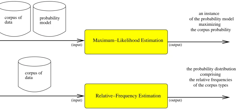
A statistics problem is a problem in which acorpus1 that has been generated in accordance with some unknownprobability distributionmust be analyzed and some type of inference about the unknown distribution must be made. In other words, in a statistics problem there is a choice between two or more probability distributions which might have generated the corpus. In practice, there are often an infinite number of different possible distributions – statisticians bundle these into one singleprobability model– which might have generated the corpus. By analyzing the corpus, an attempt is made to learn about the unknown distribution. So, on the basis of the corpus, anestimation method selects oneinstance of the probability model, thereby aiming at finding the original distribution. In this section, two common estimation methods, the relative-frequency and the maximum-likelihood estimation, are presented.
Corpora
Definition 1 Let X be a countable set. A real-valued functionf:X → R is called acorpus, if f’s values are non-negative numbers
f(x)≥0 for all x∈ X
Each x ∈ X is called a type, and each value of f is called a type frequency. The corpus size2 is defined as
|f|= X x∈X
f(x)
Finally, a corpus is callednon-empty and finite if
0<|f|<∞
In this definition, type frequencies are defined asnon-negative real numbers. The reason for not takingnatural numbers is that some statistical estimation methods define type frequencies as weighted occurrence frequencies (which are not natural but non-negative real numbers). Later on, in the context of the EM algorithm, this point will become clear. Note also that a finite corpus might consist of an infinite number of types with positive frequencies. The following definition shows that Definition 1 covers the standard notion of the term corpus
(used in Computational Linguistics) and of the termsample (used in Statistics).
Definition 2 Let x1, . . . , xn be a finite sequence of type instances from X. Each xi of this
sequence is called atoken. Theoccurrence frequencyof a typex in the sequence is defined as the following count
f(x) =| { i |xi=x} |
Obviously,f is a corpus in the sense of Definition 1, and it has the following properties: The type x does not occur in the sequence if f(x) = 0; In any other case there are f(x) tokens in the sequence which are identical to x. Moreover, the corpus size|f|is identical to n, the number of tokens in the sequence.
Relative-Frequency Estimation
Let us first present the notion of probability that we use throughout this paper.
Definition 3 Let X be a countable set of types. A real-valued functionp:X → R is called a probability distribution on X, if p has two properties: First, p’s values are non-negative numbers
p(x)≥0 for all x∈ X
and second,p’s values sum to 1
X x∈X
p(x) = 1
Readers familiar to probability theory will certainly note that we use the term probability distribution in a sloppy way (Duda et al. (2001), page 611, introduce the term probability mass function instead). Standardly, probability distributions allocate a probability value
p(A) to subsets A ⊆ X, so-called events of an event space X, such that three specific axioms are satisfied (see e.g. DeGroot (1989)):
Axiom 1 p(A)≥0 for any event A.
2Note that the corpus size|f|is well-defined: The order of summation is not relevant for the value of the (possible infinite) seriesP
x∈Xf(x), since the types are countable and the type frequencies are non-negative
probability model
data corpus of data
corpus of
comprising the probability distribution
of the corpus types the relative frequencies
Relative−Frequency Estimation Maximum−Likelihood Estimation
of the probability model maximizing the corpus probability
an instance
(output) (input)
[image:3.612.107.500.107.291.2](output) (input)
Figure 1: Maximum-likelihood estimation and relative-frequency estimation
Axiom 2 p(X) = 1.
Axiom 3 p(S∞
i=1Ai) =P∞i=1p(Ai) for any infinite sequence of disjoint events A1, A2, A3, ... Now, however, note that the probability distributions introduced in Definition 3 induce rather naturally the following probabilities for eventsA⊆ X
p(A) := X
x∈A
p(x)
Using the properties of p(x), we can easily show that the probabilities p(A) satisfy the three axioms of probability theory. So, Definition 3 is justified and thus, for the rest of the paper, we are allowed to put axiomatic probability theory out of our minds.
Definition 4 Let f be a non-empty and finite corpus. The probability distribution
˜
p:X →[0,1] where p˜(x) = f(x)
|f|
is called therelative-frequency estimate on f.
The relative-frequency estimation is the most comprehensible estimation method and has some nice properties which will be discussed in the context of the more general maximum-likelihood estimation. For now, however, note that ˜p is well defined, since both |f| > 0 and |f| < ∞. Moreover, it is easy to check that ˜p’s values sum to one: P
x∈X p˜(x) =
P
x∈X|f|−1·f(x) =|f|−1·Px∈X f(x) =|f|−1· |f|= 1.
Maximum-Likelihood Estimation
For these reasons, maximum-likelihood estimation is probably the most widely used estima-tion method.
Now, unlike relative-frequency estimation, maximum-likelihood estimation is a fully-fledged estimation method that aims at selecting an instance of a given probability model which might have originally generated the given corpus. By contrast, the relative-frequency estimate is defined on the basis of a corpus only (see Definition 4). Figure 1 reveals the conceptual difference of both estimation methods. In what follows, we will pay some attention to de-scribe the single setting, in which we are exceptionally allowed to mix up both methods (see Theorem 1). Let us start, however, by presenting the notion of a probability model.
Definition 5 A non-empty setM of probability distributions on a set X of types is called a probability model on X. The elements of Mare calledinstances of the modelM. The unrestricted probability model is the set M(X) of all probability distributions on the set of types
M(X) = (
p:X →[0,1]
X x∈X
p(x) = 1 )
A probability model M is calledrestricted in all other cases
M ⊆ M(X) and M 6=M(X)
In practice, most probability models are restricted since their instances are often defined on a setX comprising multi-dimensional types such that certain parts of the types are statistically independent (see examples 4 and 5). Here is another side note: We already checked that the relative-frequency estimate is a probability distribution, meaning in terms of Definition 5 that the relative-frequency estimate is an instance of the unrestricted probability model. So, from an extreme point of view, the relative-frequency estimation might be also regarded as a fully-fledged estimation method exploiting a corpus and a probability model (namely, the unrestricted model).
In the following, we define maximum-likelihood estimation as a method that aims at finding an instance of a given model which maximizes the probability of a given corpus. Later on, we will see that maximum-likelihood estimates have an additional property: They are the instances of the given probability model that have a “minimal distance” to the relative frequencies of the types in the corpus (see Theorem 2). So, indeed, maximum-likelihood estimates can be intuitively thought of in the intended way: They are the instances of the probability model that might have originally generated the corpus.
Definition 6 Let f be a non-empty and finite corpus on a countable set X of types. LetM
be a probability model on X. The probability of the corpus allocated by an instance p of the model M is defined as
L(f;p) = Y x∈X
p(x)f(x)
An instance pˆof the model M is called a maximum-likelihood estimate of M on f, if and only if the corpus f is allocated a maximum probability by pˆ
L(f; ˆp) = max
p∈ML(f;p)
p ~
?? ? M(X)
M
M(X) ~
p = p
M
[image:5.612.189.411.104.198.2]p ^ ^
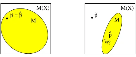
Figure 2: Maximum-likelihood estimation and relative-frequency estimation yield for some “excep-tional” probability models thesame estimate. These models are lightly restricted or even unrestricted models that contain an instance comprising the relative frequencies of all corpus types (left-hand side). In practice, however, most probability models will not behave like that. So, maximum-likelihood es-timation and relative-frequency eses-timation yield in most casesdifferent estimates. As a further and more serious consequence, the maximum-likelihood estimates have then to be searched for by genuine optimization procedures (right-hand side).
By looking at this definition, we recognize that maximum-likelihood estimates are the solu-tions of a quite complex optimization problem. So, some nasty quessolu-tions about maximum-likelihood estimation arise:
Existence Is there for any probability model and any corpus a maximum-likelihood estimate of the model on the corpus?
Uniqueness Is there for any probability model and any corpus a unique maximum-likelihood estimate of the model on the corpus?
Computability For which probability models and corpora can maximum-likelihood estimates be efficiently computed?
For some probability models M, the following theorem gives a positive answer.
Theorem 1 Let f be a non-empty and finite corpus on a countable set X of types. Then:
(i) The relative-frequency estimate p˜is a unique maximum-likelihood estimate of the unre-stricted probability model M(X) on f.
(ii) The relative-frequency estimate p˜ is a maximum-likelihood estimate of a (restricted or unrestricted) probability model Mon f, if and only if p˜is an instance of the modelM. In this case, p˜is a unique maximum-likelihood estimate of M on f.
Proof Ad (i): Combine theorems 2 and 3. Ad (ii): “⇒” is trivial. “⇐” by (i)q.e.d.
Example 1 On the basis of the following corpus
f(a) = 2, f(b) = 3, f(c) = 5
we shall calculate the maximum-likelihood estimate of the unrestricted probability model
M({a, b, c}), as well as the maximum-likelihood estimate of the restricted probability model
M=np∈ M({a, b, c})
p(a) = 0.5 o
The solution is instructive, but is left to the reader.
The Information Inequality of Information Theory
Definition 7 The relative entropy D(p || q) of the probability distribution p with respect to the probability distribution q is defined by
D(p || q) = X x∈X
p(x) logp(x)
q(x)
(Based on continuity arguments, we use the convention that 0 log0q = 0 and plogp0 =∞ and
0 log00 = 0. The logarithm is calculated with respect to the base 2.)
Connecting maximum-likelihood estimation with the concept of relative entropy, the follow-ing theorem gives the important insight that the relative-entropy of the relative-frequency estimate is minimal with respect to a maximum-likelihood estimate.
Theorem 2 Letp˜be the relative-frequency estimate on a non-empty and finite corpusf, and let Mbe a probability model on the set X of types. Then: An instance pˆof the model Mis a maximum-likelihood estimate of Mon f, if and only if the relative-entropy of p˜is minimal with respect to pˆ
D(˜p || pˆ) = min
p∈MD(˜p || p)
Proof First, the relative entropy D(˜p || p) is simply the difference of two further entropy values, the so-calledcross-entropyH(˜p;p) =−P
x∈Xp˜(x) logp(x) and theentropyH(˜p) =
−P
x∈Xp˜(x) log ˜p(x) of the relative-frequency estimate
D(˜p || p) =H(˜p;p)−H(˜p)
(Based on continuity arguments and in full agreement with the convention used in Definition 7, we use here that ˜plog 0 = −∞ and 0 log 0 = 0.) It follows that minimizing the relative entropy is equivalent to minimizing the cross-entropy (as a function of the instances p of the given probability modelM). The cross-entropy, however, is proportional to the negative log-probability of the corpusf
H(˜p;p) =− 1
So, finally, minimizing the relative entropy D(˜p || p) is equivalent to maximizing the corpus probabilityL(f;p). 3
Together with Theorem 2, the following theorem, the so-called information inequality of information theory, proves Theorem 1. The information inequality states simply that the relative entropy is a non-negative number – which is zero, if and only if the two probability distributions are equal.
Theorem 3 (Information Inequality) Let p and q be two probability distributions. Then
D(p || q)≥0
with equality if and only ifp(x) =q(x) for allx∈ X.
Proof See, e.g., Cover and Thomas (1991), page 26.
*Maximum-Entropy Estimation
Readers only interested in the expectation-maximization algorithm are encouraged to omit this section. For completeness, however, note that the relative entropy isasymmetric. That means, in general
D(p||q)6=D(q||p)
It is easy to check that the triangle inequality is not valid too. So, the relative entropyD(.||.) is not a “true” distance function. On the other hand,D(.||.) has some of the properties of a distance function. In particular, it is always non-negative and it is zero if and only ifp =q
(see Theorem 3). So far, however, we aimed at minimizing the relative entropy with respect to itssecond argument, filling the first argument slot of D(.||.) with the relative-frequency estimate ˜p. Obviously, these observations raise the question, whether it is also possible to derive other “good” estimates by minimizing the relative entropy with respect to its first argument. So, in terms of Theorem 2, it might be interesting to ask for model instances
p∗∈ M with
D(p∗||p˜) = min
p∈MD(p||p˜)
For at least two reasons, however, this initial approach of relative-entropy estimation is too simplistic. First, it is tailored to probability models that lack any generalization power. Second, it does not provide deeper insight when estimating constrained probability models. Here are the details:
3For completeness, note that the perplexityof a corpusf allocated by a model instance pis defined as perp(f;p) = 2H( ˜p;p). This yields perp(f;p) = |fq| 1
L(f;p) andL(f;p) =
1 perp(f;p)
|f|
as well as the common interpretation thatthe perplexity value measures the complexity of the given corpus from the
model instance’s view: the perplexity is equal to the size of an imaginary word list from which the corpus
• A closer look at Definition 7 reveals that the relative entropy D(p||p˜) is finite for those model instances p∈ M only that fulfill
˜
p(x) = 0⇒p(x) = 0
So, the initial approach would lead to model instances that are completely unable to generalize, since they are not allowed to allocate positive probabilities to at least some of the types not seen in the training corpus.
• Theorem 2 guarantees that the relative-frequency estimate ˜pis a solution to the initial approach of relative-entropy estimation, whenever ˜p∈ M. Now, Definition 8 introduces the constrained probability models Mconstr, and indeed, it is easy to check that ˜p is always an instance of these models. In other words, estimating constrained probability models by the approach above does not result in interesting model instances.
Clearly, all the mentioned drawbacks are due to the fact that the relative-entropy minimization is performed with respect to the relative-frequency estimate. As a resource, we switch simply to a more convenient reference distribution, thereby generalizing formally the initial problem setting. So, as the final request, we ask for model instancesp∗ ∈ Mwith
D(p∗||p0) = min
p∈MD(p||p0)
In this setting, thereference distributionp0 ∈ M(X) is a given instance of the unrestricted probability model, and from what we have seen so far,p0 should allocate all types of interest a positive probability, and moreover, p0 should not be itself an instance of the probability modelM. Indeed, this request will lead us to the interesting maximum-entropy estimates. Note first, that
D(p||p0) =H(p;p0)−H(p)
So, minimizing D(p||p0) as a function of the model instances p is equivalent to minimizing
the cross entropy H(p;p0) and simultaneously maximizing the model entropy H(p). Now, simultaneous optimization is a hard task in general, and this gives reason to focus firstly on maximizing the entropy H(p) in isolation. The following definition presents maximum-entropy estimation in terms of the well-known maximum-maximum-entropy principle (Jaynes 1957). Sloppily formulated, the maximum-entropy principle recommends to maximize the entropy
H(p) as a function of the instances pof certain “constrained” probability models.
Definition 8 Let f1, . . . , fd be a finite number of real-valued functions on a set X of types,
and finite corpus f on X. Then, the probability model constrained by the expected values of f1. . . fd on f is defined as
Mconstr= (
p∈ M(X)
Epfi=Ep˜fi for i= 1, . . . , d
)
Here, each Epfi is themodel instance’s expectation of fi
Epfi = X x∈X
p(x)fi(x)
constrained to match Ep˜fi, the observed expectation of fi
Ep˜fi = X x∈X
˜
p(x)fi(x)
Furthermore, a model instance p∗ ∈ Mconstr is called a maximum-entropy estimate of
Mconstr if and only if
H(p∗) = max
p∈Mconstr
H(p)
It is well-known that the maximum-entropy estimates have some nice properties. For example, as Definition 9 and Theorem 4 show, they can be identified to be the unique maximum-likelihood estimates of the so-called exponential models (which are also known as log-linear models).
Definition 9 Let f1, . . . , fd be a finite number of feature functions on a set X of types. The
exponential model of f1, . . . , fd is defined by
Mexp= (
p∈ M(X)
p(x) = 1
Zλ
eλ1f1(x)+...+λdfd(x) with λ
1, . . . , λd, Zλ∈ R )
Here, the normalizing constant Zλ (with λ as a short form for the sequence λ1, . . . , λd)
guarantees thatp∈ M(X), and it is given by
Zλ= X
x∈X
eλ1f1(x)+...+λdfd(x)
Theorem 4 Let f be a non-empty and finite corpus, and f1, . . . , fd be a finite number of
feature functions on a setX of types. Then
(i) The maximum-entropy estimates ofMconstr are instances of Mexp, and the
maximum-likelihood estimates of Mexp on f are instances of Mconstr.
(ii) Ifp∗ ∈ Mconstr∩ Mexp, thenp∗ is both a unique maximum-entropy estimate ofMconstr
and a unique maximum-likelihood estimate of Mexp on f.
maximum-likelihood estimation of
arbitrary probability models
exponential models
exponential models with reference distributions
⇐⇒
minimum relative-entropy estimation minimizeD(˜p||.)
(˜p=relative-frequency estimate) maximum-entropy estimation
of constrained models
minimum relative-entropy estimation of constrained models
minimizeD(.||p0)
(p0=reference distribution)
Figure 3: Maximum-likelihood estimation generalizes maximum-entropy estimation, as well as both variants of minimum relative-entropy estimation (where either the first or the second argument slot of
D(.||.) is filled by a given probability distribution).
estimate, then it is in the intersection of both models, and thus according to Part (ii), it is a unique estimate, and even more, it is both a maximum-entropy and a maximum-likelihood estimate.
Proof See e.g. Cover and Thomas (1991), pages 266-278. For an interesting alternate proof of (ii), see Ratnaparkhi (1997). Note, however, that the proof of Ratnaparkhi’s Theorem 1 is incorrect, whenever the set X of types is infinite. Although Ratnaparkhi’s proof is very elegant, it relies on the existence of a uniform distribution onX that simply does not exist in this special case. By contrast, Cover and Thomas prove Theorem 11.1.1 without using a uniform distribution onX, and so, they achieve indeed the more general result.
Finally, we are coming back to our request of minimizing the relative entropy with respect to a given reference distributionp0 ∈ M(X). For constrained probability models, the relevant results differ not much from the results described in Theorem 4. So, let
Mexp·ref = (
p∈ M(X)
p(x) = 1
Zλe
λ1f1(x)+...+λdfd(x)·p
0(x) withλ1, . . . , λd, Zλ ∈ R )
Then, along the lines of the proof of Theorem 4 it can be also proven that the following propositions are valid.
(i) The minimum relative-entropy estimates of Mconstr are instances of Mexp·ref, and the maximum-likelihood estimates of Mexp·ref on f are instances ofMconstr.
(ii) Ifp∗ ∈ Mconstr∩ Mexp·ref, thenp∗ is both a unique minimum relative-entropy estimate of Mconstr and a unique maximum-likelihood estimate of Mexp·ref onf.
All results are displayed in Figure 3.
3
The Expectation-Maximization Algorithm
of the complete−data model sequence of instances
aiming at maximizing the probability of the incomplete−data corpus
(input)
Expectation−Maximization Algorithm
(output)
symbolic analyzer
complete data
corpus
starting complete−data
model
instance incomplete−data
[image:11.612.93.512.107.236.2]incomplete data
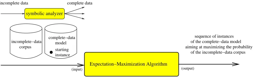
Figure 4: Input and output of the EM algorithm.
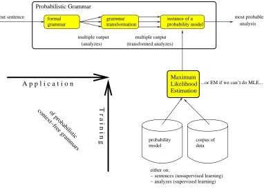
estimates for settings where this appears to be difficult if not impossible. The trick of the EM algorithm is to map the given data to complete data on which it is well-known how to perform maximum-likelihood estimation. Typically, the EM algorithm is applied in the following setting:
• Direct maximum-likelihood estimation of the given probability model on the given cor-pus is not feasible. For example, if the likelihood function is too complex (e.g. it is a product of sums).
• There is an obvious (but one-to-many) mapping to complete data, on which maximum-likelihood estimation can be easily done. The prototypical example is indeed that maximum-likelihood estimation on the complete data is already a solved problem. Both relative-frequency and maximum-likelihood estimation are common estimation methods with a two-fold input, a corpus and a probability model5 such that the instances of the model might have generated the corpus. The output of both estimation methods is simply an instance of the probability model, ideally, the unknown distribution that generated the corpus. In contrast to this setting, in which we are almost completely informed (the only thing that is not known to us is the unknown distribution that generated the corpus), the expectation-maximization algorithm is designed to estimate an instance of the probability model for settings, in which we are incompletely informed.
To be more specific, instead of acomplete-data corpus, the input of the expectation-maximization algorithm is anincomplete-data corpus together with a so-calledsymbolic analyzer. A symbolic analyzer is a device assigning to each incomplete-data type a set of analyzes, each analysis being adata type. As a result, the missing complete-data corpus can be partly compensated by the expectation-maximization algorithm: The application of the the symbolic analyzer to the incomplete-data corpus leads to anambiguous complete-data corpus. The ambiguity arises as a consequence of the inherent analytical ambiguity of the symbolic analyzer: the analyzer can replace each token of the incomplete-data corpus by a set of complete-incomplete-data types – the set of its analyzes – but clearly, the symbolic analyzer is not able to resolve the analytical ambiguity.
The expectation-maximization algorithm performs a sequence of runs over the resulting ambiguous complete-data corpus. Each of these runs consists of an expectation step fol-lowed by a maximization step. In the E step, the expectation-maximization algorithm
combines the symbolic analyzer with an instance of the probability model. The results of this combination is astatistical analyzer which is able toresolve the analytical ambi-guity introduced by the symbolic analyzer. In the M step, the expectation-maximization algorithm calculates an ordinary maximum-likelihood estimate on the resolved complete-data corpus.
In general, however, a sequence of such runs is necessary. The reason is that we never know which instance of the given probability model leads to a good statistical analyzer, and thus, which instance of the probability model shall be used in the E-step. The expectation-maximization algorithm provides a simple but somehow surprising solution to this serious problem. At the beginning, a randomly generatedstarting instanceof the given probability model is used for the first E-step. In further iterations, the estimate of the M-step is used for the next E-step. Figure 4 displays the input and the output of the EM algorithm. The procedure of the EM algorithm is displayed in Figure 5.
Symbolic and Statistical Analyzers
Definition 10 Let X andY be non-empty and countable sets. A function
A:Y →2X
is called a symbolic analyzer if the (possibly empty) sets of analyzes A(y) ⊆ X are pair-wise disjoint, and the union of all sets of analyzes A(y) is complete
X = X y∈Y
A(y)
In this case, Y is called the set of incomplete-data types, whereas X is called the set of complete-data types. So, in other words, the analyzes A(y) of the incomplete-data types y form a partition of the complete-data X. Therefore, for each x ∈ X exists a unique y ∈ Y, the so-called yield of x, such that x is an analysis of y
y=yield(x) if and only if x∈ A(y)
For example, if working in a formal-grammar framework, the grammatical sentences can be interpreted as the incomplete-data types, whereas thegrammatical analyzes of the sentences
are the complete-data types. So, in terms of Definition 10, a so-called parser – a device assigning a set of grammatical analyzes to a given sentence – is clearly a symbolic analyzer: The most important thing to check is that the parser does not assign a given grammatical analysis to two different sentences – which is pretty obvious, if the sentence words are part of the grammatical analyzes.
Definition 11 A pair <A, p >consisting of a symbolic analyzer A and a probability distri-bution p on the complete-data typesX is called a statistical analyzer. We use a statistical analyzer toinduce probabilities for the incomplete-data types y∈ Y
p(y) := X
x∈A(y)
symbolic analyzer
fq complete−data
corpus
model complete−data
M step: maximum−likelihood estimation on complete data (corpus and model) E step: generate the complete−data−corpus
expected by q
corpus incomplete−data
instance of the
q
[image:13.612.106.502.109.286.2]complete−data model (input/output)
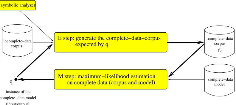
Figure 5: Procedure of the EM algorithm. An incomplete-data corpus, a symbolic analyzer (a device assigning to each incomplete-data type a set of complete-data types), and a complete-data model are given. In the E step, the EM algorithm combines the symbolic analyzer with an instanceq of the probability model. The results of this combination is a statistical analyzer that is able to resolve the ambiguity of the given incomplete data. In fact, the statistical analyzer is used to generate an expected complete-data corpusfq. In the M step, the EM algorithm calculates an ordinary maximum-likelihood estimate of the complete-data model on the complete-data corpus generated in the E step. In further iterations, the estimates of the M-steps are used in the subsequent E-steps. The output of the EM algorithm are the estimates that are produced in the M steps.
Even more important, we use a statistical analyzer toresolve the analytical ambiguity of an incomplete-data typey∈ Y by looking at theconditional probabilities of the analyzes x∈ A(y)
p(x|y) := p(x)
p(y) where y=yield(x)
It is easy to check that the statistical analyzer induces a proper probability distribution on the set Y of incomplete-data types
X y∈Y
p(y) = X
y∈Y
X x∈A(y)
p(x) = X
x∈X
p(x) = 1
Moreover, the statistical analyzer induces also proper conditional probability distributions on the sets of analyzes A(y)
X x∈A(y)
p(x|y) = X x∈A(y)
p(x)
p(y) = P
x∈A(y)p(x)
p(y) =
p(y)
p(y) = 1
Of course, by definingp(x|y) = 0 fory = yield(6 x),p(.|y) is even a probability distribution on the full setX of analyzes.
Input, Procedure, and Output of the EM Algorithm
(i) a symbolic analyzer, i.e., a function A which assigns a set of analyzes A(y)⊆ X
to each incomplete-data type y ∈ Y, such that all sets of analyzes form a partition of the set X of complete-data types
X = X y∈Y
A(y)
(ii) a non-empty and finite incomplete-data corpus, i.e., a frequency distribution f on the set of incomplete-data types
f:Y → R such that f(y)≥0 for all y∈ Y and 0<|f|<∞
(iii) a complete-data model M ⊆ M(X), i.e., each instance p ∈ M is a probability distribution on the set of complete-data types
p:X →[0,1] and X
x∈X
p(x) = 1
(*) implicit input: an incomplete-data model M ⊆ M(Y) induced by the symbolic analyzer and the complete-data model. To see this, recall Definition 11. Together with a given instance of the complete-data model, the symbolic analyzer constitutes a statistical analyzer which, in turn, induces the following instance of the incomplete-data model
p:Y →[0,1] and p(y) = X
x∈A(y)
p(x)
(Note: For both complete and incomplete data, the same notation symbols Mand pare used. The sloppy notation, however, is justified, because the incomplete-data model is a marginal of the complete-data model.)
(iv) a (randomly generated) starting instance p0 of the complete-data model M.
(Note: If permitted byM, thenp0 should not assign to anyx∈ X a probability of zero.)
Definition 13 The procedure of the EM algorithm is
(1) for each i= 1, 2, 3, ...do (2) q:=pi−1
(3) E-step: compute the complete-data corpusfq:X → R expected by q
fq(x) :=f(y)·q(x|y) where y=yield(x)
(4) M-step: compute a maximum-likelihood estimate pˆof M on fq
L(fq; ˆp) = max
p∈ML(fq, p)
(Implicit pre-condition of the EM algorithm: it exists!) (5) pi := ˆp
3
analyzes of y total frequency = f( y3 )
2
analyzes of y total frequency = f( y2 )
1
analyzes of y total frequency = f( y1 )
f
incomplete−data corpus. . .
. . .
f
qcomplete−data corpus
x x21 x22 x23
. . .
x... x31 x32 x33 . . .
x... 2
x12 x13 11
. . . x...
y1 y y3
. . .
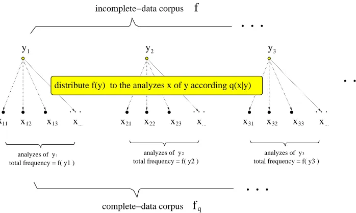
[image:15.612.126.475.106.315.2]distribute f(y) to the analyzes x of y according q(x|y)
Figure 6: The E step of the EM algorithm. A complete-data corpusfq(x) is generated on the basis of the incomplete-data corpus f(y) and the conditional probabilitiesq(x|y) of the analyzes ofy. The frequency f(y) is distributed among the complete-data types x∈ A(y) according to the conditional probabilitiesq(x|y). A simple reversed procedure guarantees that the original incomplete-data corpus
f(y) can be recovered from the generated corpusfq(x): Sum up all frequenciesfq(x) with x∈ A(y). So the size of both corpora is the same|fq|=|f|. Memory hook: fq is theqomplete data corpus.
In line (3) of the EM procedure, a complete-data corpusfq(x) has to be generated on the basis of the incomplete-data corpusf(y) and the conditional probabilitiesq(x|y) of the analyzes ofy
(conditional probabilities are introduced in Definition 11). In fact, this generation procedure is conceptually very easy: according to the conditional probabilities q(x|y), the frequency
f(y) has to be distributed among the complete-data types x ∈ A(y). Figure 6 displays the procedure. Moreover, there exists a simple reversed procedure (summation of all frequencies
fq(x) with x ∈ A(y)) which guarantees that the original corpusf(y) can be recovered from the generated corpus fq(x). Finally, the size of both corpora is the same
|fq|=|f|
In line (4) of the EM procedure, it is stated that a maximum-likelihood estimate ˆp of the complete-data model has to be computed on the complete-data corpus fq expected by q. Recall for this purpose that the probability of fq allocated by an instancep ∈ Mis defined as
L(fq;p) = Y x∈X
p(x)fq(x)
In contrast, the probability of the incomplete-data corpusf allocated by an instancepof the incomplete-data model is much more complex. Using Definition 12.*, we get an expression involving a product of sums
L(f;p) = Y y∈Y
X x∈A(y)
p(x)
Nevertheless, the following theorem reveals that the EM algorithm aims at finding an instance of the incomplete-data model which possibly maximizes the probability of the incomplete-data corpus.
Theorem 5 The output of the EM algorithm is: A sequence of instances of the complete-data modelM, the so-called EM re-estimates,
p0, p1, p2, p3, ...
such that the sequence of probabilities allocated to the incomplete-data corpus is monotonic increasing
L(f;p0)≤L(f;p1)≤L(f;p2)≤L(f;p3)≤. . .
It is common wisdom that the sequence of EM re-estimates will converge to a (local) maximum-likelihood estimate of the incomplete-data model on the incomplete-data corpus. As proven by Wu (1983), however, the EM algorithm will do this only in specific circumstances. Of course, it is guaranteed that the sequence of corpus probabilities (allocated by the EM re-estimates) must converge. However, we are more interested in the behavior of the EM re-estimates itself. Now, intuitively, the EM algorithm might get stuck in a saddle point or even a local mini-mum of the corpus-probability function, whereas the associated model instances are hopping uncontrolled around (for example, on a circle-like path in the “space” of all model instances).
Proof See theorems 6 and 7.
The Generalized Expectation-Maximization Algorithm
The EM algorithm performs a sequence of maximum-likelihood estimations on complete data, resulting in good re-estimates on incomplete-data (“good” in the sense of Theorem 5). The following theorem, however, reveals that the EM algorithm might overdo it somehow, since there exist alternative M-steps which can be easier performed, and which result in re-estimates having the same property as the EM re-estimates.
Definition 14 A generalized expectation-maximization (GEM) algorithm has exactly the same input as the EM-algorithm, but an easier M-step is performed in its procedure:
(4) M-step (GEM):compute an instancepˆof the complete-data modelMsuch that
L(fq; ˆp)≥L(fq;q)
Theorem 6 The output of a GEM algorithm is: A sequence of instances of the complete-data modelM, the so-calledGEM re-estimates, such that the sequence of probabilities allocated to the incomplete-data corpus is monotonic increasing.
Proof Various proofs have been given in the literature. The first one was presented by
Dempster et al. (1977). For other variants of the EM algorithm, the book of McLachlan and Krishnan (1997) is a good source. Here, we present something along the lines of the original proof. Clearly,
which are involved in the M-steps of the GEM algorithm (where both types of corpora are allocated a probability by the same instance p of the modelM). A certain entity, which we would like to call the expected cross-entropy on the analyzes, plays a major role for solving this task. To be specific, the expected cross-entropy on the analyzes is defined as the expectation of certain cross-entropy values HA(y)(q, p) which are calculated on the different sets A(y) of analyzes. Then, of course, the “expectation” is calculated on the basis of the relative-frequency estimate ˜p of the given incomplete-data corpus
HA(q;p) =
X y∈Y
˜
p(y)·HA(y)(q;p)
Now, for two instances q and p of the complete-data model, their conditional probabilities
q(x|y) and p(x|y) form proper probability distributions on the set A(y) of analyzes ofy (see Definition 11). So, the cross-entropy HA(y)(q;p) on the set A(y) is simply given by
HA(y)(q;p) =− X
x∈A(y)
q(x|y) logp(x|y)
Recalling the central task of this proof, a bunch of relatively straight-forward calculations leads to the following interesting equation6
L(f;p) =2HA(q;p)|f|·L(f
q;p) Using this equation, we can state that
L(f;p)
L(f;q) =
2HA(q;p)−HA(q,q)|f|·L(fq;p)
L(fq;q)
In what follows, we will show that, after each M-step of a GEM algorithm (i.e. forp being a GEM re-estimate ˆp), both of the factors on the right-hand side of this equation are not less than one. First, an iterated application of the information inequality of information theory (see Theorem 3) yields
HA(q;p)−HA(q, q) =
X y∈Y
˜
p(y)·HA(y)(q;p)−HA(y)(q;q)
= X
y∈Y
˜
p(y)·DA(y)(q||p)
≥ 0
6It is easier to show that
H(˜p;p) =H(˜pq;p)−HA(q;p).
Here, ˜pis the relative-frequency estimate on the incomplete-data corpusf, whereas ˜pqis the relative-frequency estimate on the complete-data corpus fq. However, by defining an “average perplexity of the analyzes”, perpA(q;p) := 2HA(q;p)(see also Footnote 3), the true spirit of the equation can be revealed:
L(fq;p) =L(f;p)·
1 perpA(q;p)
|f|
So, the first factor is never (i.e. for no model instancep) less than one
2HA(q;p)−HA(q,q)|f|≥1
Second, by definition of the M-step of a GEM algorithm, the second factor is also not less than one
L(fq; ˆp)
L(fq;q)
≥1 So, it follows
L(f; ˆp)
L(f;q) ≥1
yielding that the probability of the incomplete-data corpus allocated by the GEM re-estimate ˆ
pis not less than the probability of the incomplete-data corpus allocated by the model instance
q (which is either the starting instancep0 of the GEM algorithm or the previously calculated GEM re-estimate)
L(f; ˆp)≥L(f;q) Theorem 7 An EM algorithm is a GEM algorithm.
Proof In the M-step of an EM algorithm, a model instance ˆp is selected such that
L(fq; ˆp) = max
p∈ML(fq, p)
So, especially
L(fq; ˆp)≥L(fq, q)
and the requirements of the M-step of a GEM algorithm are met.
4
Rolling Two Dice
Example 2 We shall now consider an experiment in which two loaded dice are rolled, and we shall compute the relative-frequency estimate on a corpus of outcomes.
If we assume that the two dice are distinguishable, each outcome can be represented as a pair of numbers (x1, x2), where x1 is the number that appears on the first die and x2 is the number that appears on the second die. So, for this experiment, an appropriate set X of types comprises the following 36 outcomes:
(x1, x2) x2= 1 x2 = 2 x2= 3 x2 = 4 x2 = 5 x2= 6
x1 = 1 (1,1) (1,2) (1,3) (1,4) (1,5) (1,6)
x1 = 2 (2,1) (2,2) (2,3) (2,4) (2,5) (2,6)
x1 = 3 (3,1) (3,2) (3,3) (3,4) (3,5) (3,6)
x1 = 4 (4,1) (4,2) (4,3) (4,4) (4,5) (4,6)
x1 = 5 (5,1) (5,2) (5,3) (5,4) (5,5) (5,6)
If we throw the two dice a 100 000 times, then the following occurrence frequencies might arise
f(x1, x2) x2= 1 x2 = 2 x2= 3 x2= 4 x2 = 5 x2= 6
x1 = 1 3790 3773 1520 1498 2233 2298
x1 = 2 3735 3794 1497 1462 2269 2184
x1 = 3 4903 4956 1969 2035 2883 3010
x1 = 4 2495 2519 1026 1049 1487 1451
x1 = 5 3820 3735 1517 1498 2276 2191
x1 = 6 6369 6290 2600 2510 3685 3673
The size of this corpus is |f|= 100 000. So, the relative-frequency estimate ˜p on f can be easily computed (see Definition 4)
˜
p(x1, x2) x2 = 1 x2 = 2 x2 = 3 x2= 4 x2 = 5 x2 = 6
x1= 1 0.03790 0.03773 0.01520 0.01498 0.02233 0.02298
x1= 2 0.03735 0.03794 0.01497 0.01462 0.02269 0.02184
x1= 3 0.04903 0.04956 0.01969 0.02035 0.02883 0.03010
x1= 4 0.02495 0.02519 0.01026 0.01049 0.01487 0.01451
x1= 5 0.03820 0.03735 0.01517 0.01498 0.02276 0.02191
x1= 6 0.06369 0.06290 0.02600 0.02510 0.03685 0.03673
Example 3 We shall consider again Experiment 2 in which two loaded dice are rolled, but we shall now compute the relative-frequency estimate on the corpus of outcomes of the first die, as well as on the corpus of outcomes of the second die.
If we look at the same corpus as in Example 2, then the corpus f1 of outcomes of the first die can be calculated asf1(x1) =P
x2f(x1, x2). An analog summation yields the corpus of
outcomes of the second die, f2(x2) = Px1f(x1, x2). Obviously, the sizes of all corpora are
identical |f1|=|f2|=|f|= 100 000. So, the relative-frequency estimates ˜p1 on f1 and ˜p2 on
f2 are calculated as follows
f1(x1) x1 15112 1 14941 2 19756 3 10027 4 15037 5 25127 6
˜
p1(x1) x1 0.15112 1 0.14941 2 0.19756 3 0.10027 4 0.15037 5 0.25127 6
f2(x2) x2 25112 1 25067 2 10129 3 10052 4 14833 5 14807 6
˜
p2(x2) x2 0.25112 1 0.25067 2 0.10129 3 0.10052 4 0.14833 5 0.14807 6
Example 4 We shall consider again Experiment 2 in which two loaded dice are rolled, but we shall now compute a maximum-likelihood estimate of the probability model which assumes that the numbers appearing on the first and second die are statistically independent.
First, recall the definition of statistical independence (see e.g. Duda et al. (2001), page 613).
Definition 15 The variables x1 and x2 are said to be statistically independent given a
joint probability distribution p on X if and only if
where p1 and p2 are the marginal distributions for x1 and x2
p1(x1) =X x2
p(x1, x2)
p2(x2) =X x1
p(x1, x2)
So, letM1/2 be the probability model which assumes that the numbers appearing on the first and second die are statistically independent
M1/2 ={p∈ M(X) |x1 and x2 are statistically independent given p}
In Example 2, we have calculated the relative-frequency estimator ˜p. Theorem 1 states that ˜p
is the unique maximum-likelihood estimate of the unrestricted modelM(X). Thus, ˜pis also a candidate for a maximum-likelihood estimate ofM1/2. Unfortunately, however,x1 andx2are notstatistically independent given ˜p(see e.g. ˜p(1,1) = 0.03790 and ˜p1(1)·p˜2(1) = 0.0379493). This has two consequences for the experiment in which two (loaded) dice are rolled:
• the probability model, which assumes that the numbers appearing on the first and second die are statistically independent, is arestricted model (see Definition 5), and
• the relative-frequency estimate is in general not a maximum-likelihood esti-mate of the standard probability model assuming that the numbers appearing on the first and second die are statistically independent.
Therefore, we are now following Definition 6 to compute the maximum-likelihood estimate of M1/2. Using the independence property, the probability of the corpus f allocated by an instance p of the modelM1/2 can be calculated as
L(f;p) =
Y x1=1,...,6
p1(x1)f1(x1) ·
Y x2=1,...,6
p2(x2)f2(x2)
=L(f1;p1)·L(f2;p2)
Definition 6 states that the maximum-likelihood estimate ˆp of M1/2 on f must maximize
L(f;p). A product, however, is maximized, if and only if its factors are simultaneously maximized. Theorem 1 states that the corpus probabilities L(fi;pi) are maximized by the relative-frequency estimators ˜pi. Therefore, the product of the relative-frequency estimators
˜
p1 and ˜p2 (on f1 and f2 respectively) might be a candidate for the maximum-likelihood estimate ˆp we are looking for
ˆ
p(x1, x2) = ˜p1(x1)·p˜2(x2)
Now, note that the marginal distributions of ˆp are identical with the relative-frequency esti-mators on f1 and f2. For example, ˆp’s marginal distribution for x1 is calculated as
ˆ
p1(x1) =X x2
ˆ
p(x1, x2) =X x2
˜
p1(x1)·p˜2(x2) = ˜p1(x1)·X
x2
˜
p2(x2) = ˜p1(x1)·1 = ˜p1(x1)
A similar calculation yields ˆp2(x2) = ˜p2(x2). Both equations state that x1 andx2 are indeed statistically independent given ˆp
ˆ
So, finally, it is guaranteed that ˆp is an instance of the probability model M1/2 as required for a maximum-likelihood estimate of M1/2. Note: pˆis even an unique maximum-likelihood
estimate since the relative-frequency estimates p˜i are unique maximum-likelihood estimates
(see Theorem 1). The relative-frequency estimates ˜p1 and ˜p2 have already been calculated in Example 3. So, ˆpis calculated as follows
ˆ
p(x1, x2) x2 = 1 x2 = 2 x2 = 3 x2 = 4 x2 = 5 x2 = 6
x1= 1 0.0379493 0.0378813 0.0153069 0.0151906 0.0224156 0.0223763
x1= 2 0.0375198 0.0374526 0.0151337 0.0150187 0.022162 0.0221231
x1= 3 0.0496113 0.0495224 0.0200109 0.0198587 0.0293041 0.0292527
x1= 4 0.0251798 0.0251347 0.0101563 0.0100791 0.014873 0.014847
x1= 5 0.0377609 0.0376932 0.015231 0.0151152 0.0223044 0.0222653
x1= 6 0.0630989 0.0629859 0.0254511 0.0252577 0.0372709 0.0372055 Example 5 We shall consider again Experiment 2 in which two loaded dice are rolled. Now, however, we shall assume that we are incompletely informed: the corpus of outcomes (which is given to us) consists only of the sums of the numbers which appear on the first and second die. Nevertheless, we shall compute an estimate for a probability model on the complete-data
(x1, x2)∈ X.
If we assume that the corpus which is given to us was calculated on the basis of the corpus given in Example 2, then the occurrence frequency of a sum y can be calculated as f(y) = P
x1+x2=yf(x1, x2). These numbers are displayed in the following table
f(y) y
3790 2 7508 3 10217 4 10446 5 12003 6 17732 7 13923 8 8595 9 6237 10 5876 11 3673 12 For example,
f(4) = f(1,3) +f(2,2) +f(3,1) = 1520 + 3794 + 4903 = 10217
The problem is now, whether this corpus of sums can be used to calculate a good esti-mate on the outcomes (x1, x2) itself. Hint: Examples 2 and 4 have shown that a unique relative-frequency estimate p˜(x1, x2)and a unique maximum-likelihood estimate pˆ(x1, x2) can
be calculated on the basis of the corpus f(x1, x2). However, right now, this corpus is not
available! Putting the example in the framework of the EM algorithm (see Definition 12), the set of incomplete-data typesis
whereas the set ofcomplete-data typesisX. We also know theset of analyzes for each incomplete-data typey∈ Y
A(y) ={(x1, x2)∈ X | x1+x2=y}
As in Example 4, we are especially interested in an estimate of the (slightly restricted) complete-data model M1/2 which assumes that the numbers appearing on the first and second die are statistically independent. So, for this case, a randomly generatedstarting in-stance p0(x1, x2) of the complete-data model is simply the product of a randomly generated probability distributionp01(x1) for the numbers appearing on the first dice, and a randomly generated probability distribution p02(x2) for the numbers appearing on the second dice
p0(x1, x2) =p01(x1)·p02(x2)
The following tables display some randomly generated numbers for p01 and p02
p01(x1) x1
0.18 1 0.19 2 0.16 3 0.13 4 0.17 5 0.17 6
p02(x2) x2
0.22 1 0.23 2 0.13 3 0.16 4 0.14 5 0.12 6
Using the random numbers forp01(x1) andp02(x2), a starting instancep0of the complete-data modelM1/2 is calculated as follows
p0(x1, x2) x2= 1 x2 = 2 x2 = 3 x2= 4 x2 = 5 x2 = 6
x1 = 1 0.0396 0.0414 0.0234 0.0288 0.0252 0.0216
x1 = 2 0.0418 0.0437 0.0247 0.0304 0.0266 0.0228
x1 = 3 0.0352 0.0368 0.0208 0.0256 0.0224 0.0192
x1 = 4 0.0286 0.0299 0.0169 0.0208 0.0182 0.0156
x1 = 5 0.0374 0.0391 0.0221 0.0272 0.0238 0.0204
x1 = 6 0.0374 0.0391 0.0221 0.0272 0.0238 0.0204 For example,
p0(1,3) = p01(1)·p02(3) = 0.18·0.13 = 0.0234
p0(2,2) = p01(2)·p02(2) = 0.19·0.23 = 0.0437
p0(3,1) = p01(3)·p02(1) = 0.16·0.22 = 0.0352
So, we are ready to start the procedure of the EM algorithm.
First EM iteration. In the E-step, we shall compute the complete-data corpus fq
expected byq :=p0. For this purpose, the probability of each incomplete-data type given the starting instance p0 of the complete-data model has to be computed (see Definition 12.*)
p0(y) = X x1+x2=y
The above displayed numbers forp0(x1, x2) yield the following instance of the incomplete-data model
p0(y) y
0.0396 2 0.0832 3 0.1023 4 0.1189 5 0.1437 6 0.1672 7 0.1272 8 0.0867 9 0.0666 10 0.0442 11 0.0204 12 For example,
p0(4) = p0(1,3) +p0(2,2) +p0(3,1) = 0.0234 + 0.0437 + 0.0352 = 0.1023
So, the complete-data corpus expected byq :=p0 is calculated as follows (see line (3) of the EM procedure given in Definition 13)
fq(x1, x2) x2= 1 x2 = 2 x2= 3 x2 = 4 x2 = 5 x2= 6
x1= 1 3790 3735.95 2337.03 2530.23 2104.91 2290.74
x1= 2 3772.05 4364.45 2170.03 2539.26 2821 2495.63
x1= 3 3515.53 3233.08 1737.39 2714.95 2451.85 1903.39
x1= 4 2512.66 2497.49 1792.29 2276.72 1804.26 1460.92
x1= 5 3123.95 4146.66 2419.01 2696.47 2228.84 2712
x1= 6 3966.37 4279.79 2190.88 2547.24 3164 3673 For example,
fq(1,3) = f(4)·
p0(1,3)
p0(4)
= 10217·0.0234
0.1023 = 2337.03
fq(2,2) = f(4)·
p0(2,2)
p0(4)
= 10217·0.0437
0.1023 = 4364.45
fq(3,1) = f(4)·
p0(3,1)
p0(4) = 10217· 0.0352
0.1023 = 3515.53
(The frequency f(4) of the dice sum 4 is distributed to its analyzes (1,3), (2,2), and (3,1), simply by correlating the current probabilitiesq =p0 of the analyses...)
complete-data corpusfq (where currently q=p0), the corpusfq1 of outcomes of the first die is calculated asfq1(x1) =P
x2fq(x1, x2), whereas the corpus of outcomes of the second die is
calculated as fq2(x2) =Px1fq(x1, x2). The following tables display them: fq1(x1) x1
16788.86 1 18162.42 2 15556.19 3 12344.34 4 17326.93 5 19821.28 6
fq2(x2) x2 20680.56 1 22257.42 2 12646.63 3 15304.87 4 14574.86 5 14535.68 6 For example,
fq1(1) = fq(1,1) +fq(1,2) +fq(1,3) +fq(1,4) +fq(1,5) +fq(1,6)
= 3790 + 3735.95 + 2337.03 + 2530.23 + 2104.91 + 2290.74 = 16788.86
fq2(1) = fq(1,1) +fq(2,1) +fq(3,1) +fq(4,1) +fq(5,1) +fq(6,1)
= 3790 + 3772.05 + 3515.53 + 2512.66 + 3123.95 + 3966.37 = 20680.56 The sizes of both corpora are still |fq1| = |fq2| = |f| = 100 000, resulting in the following relative-frequency estimates (p11 on fq1 respectivelyp12 on fq2)
p11(x1) x1 0.167889 1 0.181624 2 0.155562 3 0.123443 4 0.173269 5 0.198213 6
p12(x2) x2 0.206806 1 0.222574 2 0.126466 3 0.153049 4 0.145749 5 0.145357 6
So, the following instance is the maximum-likelihood estimate of the modelM1/2 on fq
p1(x1, x2) x2= 1 x2= 2 x2= 3 x2= 4 x2= 5 x2= 6
x1= 1 0.0347204 0.0373677 0.0212322 0.0256952 0.0244696 0.0244038
x1= 2 0.0375609 0.0404247 0.0229692 0.0277973 0.0264715 0.0264003
x1= 3 0.0321711 0.034624 0.0196733 0.0238086 0.022673 0.022612
x1= 4 0.0255287 0.0274752 0.0156113 0.0188928 0.0179917 0.0179433
x1= 5 0.035833 0.0385651 0.0219126 0.0265186 0.0252538 0.0251858
x1= 6 0.0409916 0.044117 0.0250672 0.0303363 0.0288893 0.0288116 For example,
p1(1,1) = p11(1)·p12(1) = 0.167889·0.206806 = 0.0347204
p1(1,2) = p11(1)·p12(2) = 0.167889·0.222574 = 0.0373677
p1(2,1) = p11(2)·p12(1) = 0.181624·0.206806 = 0.0375609
p1(2,2) = p11(2)·p12(2) = 0.181624·0.222574 = 0.0404247
1584th EM iteration. The estimate which is calculated here is
p1584,1(x1) x1 0.158396 1 0.141282 2 0.204291 3 0.0785532 4 0.172207 5 0.24527 6
p1584,2(x2) x2 0.239281 1 0.260559 2 0.104026 3 0.111957 4 0.134419 5 0.149758 6 yielding
p1584(x1, x2) x2 = 1 x2 = 2 x2 = 3 x2 = 4 x2 = 5 x2 = 6
x1 = 1 0.0379012 0.0412715 0.0164773 0.0177336 0.0212914 0.0237211
x1 = 2 0.0338061 0.0368123 0.014697 0.0158175 0.018991 0.0211581
x1 = 3 0.048883 0.0532299 0.0212516 0.0228718 0.0274606 0.0305942
x1 = 4 0.0187963 0.0204678 0.00817158 0.00879459 0.0105591 0.011764
x1 = 5 0.0412059 0.0448701 0.017914 0.0192798 0.0231479 0.0257894
x1 = 6 0.0586885 0.0639074 0.0255145 0.0274597 0.032969 0.0367312 In this example, more EM iterations will result in exactly the same re-estimates. So, this is a strong reason to quit the EM procedure. Comparing p1584,1 and p1584,2 with the results of Example 3(Hint: where we have assumed that a complete-data corpus is given to us!), we see that the EM algorithm yields pretty similar estimates.
5
Probabilistic Context-Free Grammars
This Section provides a more substantial example based on the context-free grammar or CFGformalism, and it is organized as follows: First, we will give some background informa-tion about CFGs, thereby motivating that treating CFGs as generators leads quite naturally to the notion of a probabilistic context-free grammar (PCFG). Second, we provide some ad-ditional background information about ambiguity resolution by probabilistic CFGs, thereby focusing on the fact that probabilistic CFGs can resolve ambiguities, if the underlying CFG has a sufficiently high expressive power. For other cases, we are pin-pointing to some use-ful grammar-transformation techniques. Third, we will investigate the standard probability model of CFGs, thereby proving that this model is restricted in almost all cases of inter-est. Furthermore, we will give a new formal proof that maximum-likelihood estimation of a CFG’s probability model on a corpus of trees is equal to the well-known and especially simple treebank-training method. Finally, we will present the EM algorithm for training a (manually written) CFG on a corpus of sentences, thereby pin-pointing to the fact that EM training simply consists of an iterative sequence of treebank-training steps. Small toy examples will accompany all proofs that are given in this Section.
Background: Probabilistic Modeling of CFGs
separated by a special symbol “ −→ ”, the so-called rewriting symbol. The two parts of a rule are made up of so-called terminal and non-terminal symbols: a rule’s left-hand side simply consists of a single non-terminal symbol, whereas the right-hand side is a finite sequence of terminal and non-terminal symbols7. Finally, the set of non-terminal symbols contains at least one so-called starting symbol. CFGs are also called phrase-structure grammars, and the formalism is equivalent to Backus-Naur forms or BNF introduced by Backus (1959). In computational linguistics, a CFG is usually used in two ways
• as a generator: a device for generating sentences, or
• as a parser: a device for assigning structure to a given sentence
In the following, we will briefly discuss these two issues. First of all, note that in natural language, words do not occur in any order. Instead, languages have constraints on word order8. The central idea underlying phrase-structure grammars is that words are organized intophrases, i.e., grouping of words that form a unit. Phrases can be detected, for example, by their ability (i) to stand alone (e.g. as an answer of a wh-question), (ii) to occur in various sentence positions, or by their ability (iii) to show uniform syntactic possibilities for expansion or substitution. As an example, here is the very first context-free grammar parse tree presented by Chomsky (1956):
Sentence
NP the man
VP Verb took
NP the book
As being displayed, Chomsky identified for the sentence “the man took the book” (encoded in the leaf nodes of the parse tree) the following phrases: two noun phrases, “the man” and “the book” (the figure displays them as NP subtrees), and oneverb phrase, “took the book” (displayed as VP subtree). The following list of sentences, where these three phrases have been substituted or expanded, bears some evidence for Chomsky’s analysis:
he the man the tall man the very tall man the tall man with sad eyes
took
it the book the interesting book the very interesting book the very interesting book with 934 pages
Chomsky’s parse tree is based on the following CFG: Sentence −→ NP VP NP −→ the man NP −→ the book VP −→ Verb NP Verb −→ took
The CFG’s terminal symbols are {the, man, took, book}, its non-terminal symbols are
{Sentence, NP, VP, Verb}, and its starting symbol is “Sentence”. Now, we are coming back to the beginning of the section, where we mentioned that a CFG is usually thought of in two ways: as a generatoror as a parser. As a generator, the example CFG might produce the following series of intermediate parse trees (only the last one will be submitted to the generator’s output):
Sentence Sentence NP VP
Sentence NP the man
VP
Sentence
NP the man
VP Verb NP Sentence
NP the man
VP Verb took
NP
Sentence
NP the man
VP Verb took
NP the book
Starting with the starting symbol, each of these intermediate parse trees is generated by applying one rule of the CFG to a suitable non-terminal leaf node of the previous parse tree, thereby adding the CFG rule as a local tree. The generator stops, if all leaf nodes of the current parse tree are terminal nodes. The whole generation process, of course, is non-deterministic, and this fact will lead us later on directly to probabilistic CFGs. As a parser, instead, the example CFG has to deal with an input sentence like
“the man took the book”
Usually, the parser starts processing the input sentence by assigning the words some local trees:
NP the man
Verb took
NP the book
Then, the parser tries to add more local trees, by processing all the non-terminal nodes found in previous steps:
NP the man
VP Verb took
NP the book
Doing this recursively, the parser provides us with a parse tree of the input sentence: Sentence
NP the man
VP Verb took
NP the book
Now, we demonstrate that the fact that we can understand CFGs as generators leads directly to theprobabilistic context-free grammar orPCFGformalism. As we already demonstrated for the generation process, the rules of the CFG serve as local trees that are incrementally used to build up a full parse tree (i.e. a parse tree without any non-terminal leaf nodes). This process, however, is non-deterministic: At most of its steps, some sort of random choiceis involved that selects one of the different CFG rules which can potentially be appended to one of the non-terminal leaf nodes of the current parse tree9. Here is an example in the context of the generation process displayed above. For the CFG underlying Chomsky’s very first parse tree, the non-terminal symbol NP is the left-hand side of two rules:
NP −→ the man NP −→ the book
Clearly, when using the underlying CFG as a generator, we have to select either the first or the second rule, whenever a local NP tree shall be appended to the partial-parse tree given in the actual generation step. The choice might be either fair (both rules are chosen with probability 0.5) orunfair(the first rule is chosen, for example, with probability 0.9 and the second one with probability 0.1). In either case, a random choice between competing rules can be described by probability values which are directly allocated to the rules:
0≤p(NP −→the man)≤1 and 0≤p(NP −→the book)≤1 such that
p(NP −→the man) + p(NP −→the book) = 1
Now, having these probabilities at hand, it turns out that it is even possible to predict how often the generator will produce the one or the other of the following alternate partial-parse trees:
Sentence
NP the man
VP Verb took
NP
Sentence
NP the book
VP Verb took
NP
p(NP −→the man)·100% p(NP −→the book)·100%
In turn, having this result at hand, we can also predict how often the generator will produce full-parse trees, for example, Chomsky’s very first parse tree, or the parse tree of the sentence “the book took the book”:
Sentence
NP the man
VP Verb took
NP the book
Sentence
NP the book
VP Verb took
NP the book
p(NP −→the man)·p(NP −→the book)·100% p(NP −→the book)·p(NP −→the book)·100%
So, if p(NP −→the man) = 0.9 and p(NP −→the book) = 0.1, then it is nine times more likely that the generator produces Chomsky’s very first parse tree. In the following, we are trying to generalize this result even a bit more. As we saw, there are three rules in the CFG, which cause no problems in terms of uncertainty. These are:
Sentence −→ NP VP VP −→ Verb NP Verb −→ took
To be more specific, we saw that these three rules have been always deterministically added to the partial-parse trees of the generation process. In terms of probability theory, determinism is expressed by the fact that certain events occur with a probability of one. In other words, a generator selects each of these rules with a probability of 100%, either when starting the generation process, or when expanding a VP or a Verb non-terminal node. So, we let
p(Sentence −→NP VP) = 1
p(VP −→Verb NP) = 1 p(Verb −→took) = 1
The question is now: Have we won something by treating also the deterministic choices as probabilistic events? The answer is yes: A closer look at our example reveals that we can now predict easily how often the generator will produce a specific parse tree: The likelihood of a CFG’s parse tree can be simply calculated as the product of the probabilities of all rules occurring in the tree. For example:
Sentence
NP the man
VP Verb took
NP the book
p(S −→NP VP)·p(NP −→the man)·p(VP −→Verb NP)·p(Verb −→took)·p(NP −→the book)
CFG rule Rule probability Sentence −→ NP VP p(Sentence −→NP VP) = 1
NP −→ the man NP −→ the book
p(NP −→the man)
p(NP −→the book) )
summing to 1
VP −→ Verb NP p(VP −→Verb NP) = 1 Verb −→ took p(Verb −→took) = 1
As a result, the likelihood of each of the grammar’s parse trees (when using the CFG as a generator) can be calculated by multiplying the probabilities of all rules occurring in the tree. This observation leads directly to the standard definition of a probabilistic context-free grammar, as well as to the definition of probabilities for parse-trees.
Definition 16 A pair < G, p >consisting of a context-free grammar G and a probability dis-tributionp:X →[0,1]on the set X of all finite full-parse trees ofGis called a probabilistic context-free grammar or PCFG, if for all parse treesx∈ X
p(x) = Y r∈G
p(r)fr(x)
Here, fr(x) is the number of occurrences of the ruler in the tree x, and p(r) is a probability
allocated to the rule r, such that for all non-terminal symbols A
X r∈GA
p(r) = 1
where GA = { r ∈G |lhs(r) =A} is the grammar fragment comprising all rules with the
left-hand side A. In other words, a probabilistic free grammar is defined by a context-free grammar G and some probability distributions on the grammar fragments GA, thereby
inducing a probability distribution on the set of all full-parse trees.
So far, we have not checked for our example that the probabilities of all full-parse trees are summing up to one. According to Definition 16, however, this isthe fundamental property of PCFGs (and it should be really checked for every PCFG which is accidentally given to us). Obviously, the example grammar has four full-parse trees, and the sum of their probabilities can be calculated as follows (by omitting all rules with a probability of one):
p(X) = p(NP −→the man)·p(NP −→the book) +
p(NP −→the book)·p(NP −→the book) +
p(NP −→the man)·p(NP −→the man) +
p(NP −→the book)·p(NP −→the man) = p(NP −→the man) +p(NP −→the book)
·p(NP −→the book) +
p(NP −→the man) +p(NP −→the book)
·p(NP −→the man) = 1
S −→ NP sleeps (1.0) S −→ John sleeps (0.7) NP −→ John (0.3)
The second one is a well-known highly-recursive grammar (Chi and Geman 1998), and it is given by
S −→ S S (q)
S −→ a (1-q) with 0.5< q≤1
What is wrong with these grammars? Well, the first grammar provides us with a probability distribution on its full-parse trees, as can be seen here
S NP John
sleeps
S John sleeps 1.0·0.3 = 0.3 0.7
On each of its grammar fragments, however, the rule probabilities do not form a probability distribution (neither onGS nor on GNP). The second grammar is even worse: We do have a probability distribution on GS, but even so, we do not have a probability distribution on the set of full-parse trees (because their probabilities are summing to less than one10).
10This can be proven as follows: LetT be the set of all finite full-parse trees that can be generated by the given context-free grammar. Then, it is easy to verify thatπ:=p(T) is a solution of the following equation
π= 1−q+q·π·π Here, 1−qis the probability of the tree S
a
, whereasq·π·πcorresponds to the forest S
T T
.
It is easy to check that the derived quadratic equation has two solutions: π1= 1 andπ2 =1−qq. Note that it is quite natural thattwosolutions arise: The set of all “infinite full-parse trees” matches also our under-specified approach of calculatingπ. Now, in the case of 0.5< q≤1, it turns out that the set of infinite trees is allocated a proper probability π1 = 1. (For the special caseq = 1, this can be intuitively verified: The generator will never touch the rule S −→ a , and therefore, this special PCFG produces infinite parse trees only.) As a consequence, all finite full-parse trees is allocated the total probabilityπ2. In other words,p(T) = 1−qq <1. In a certain sense, however, we are able to repair both grammars. For example,
S −→NP sleeps (0.3) S −→John sleeps (0.7) NP −→John (1.0) is the standard-PCFG counterpart of the first grammar, where
S −→S S (1-q)
S −→a (q) with 0.5< q≤1
is a standard-PCFG counterpart of the second grammar: The first grammar and its counterpart provide us with exactly the same parse-tree probabilities, while the second grammar and its counterpart produce parse-tree probabilities, which are proportional to each other. Especially for the second example, this interesting result is a special case of an important general theorem recently proven by Nederhof and Satta (2003). Sloppily formulated, their Theorem 7 states that: For each weighted CFG (defined on the basis of rule weights instead of rule probabilities) is a standard PCFG with the same symbolic backbone, such that (i) the parse-tree probabilities (produced by the PCFG) are summing to one, and (ii) the parse-tree weights (produced by the weighted CFG) are proportional to the parse-tree probabilities (produced by the PCFG).