Article
Electrical Capacitance Volume Tomography
Validation of Column Flotation Process with Gas
Injection Variation
Sri Harjanto
1,a,*, Didied Haryono
1,2,b, Hermansyah Emir Faisal
2, Kholis Daniah
2,
Harisma Nugraha
3, Mahfudz Al Huda
3, and Warsito P. Taruno
31 Department of Metallurgical and Material Engineering, Universitas Indonesia, Depok, Indonesia
2 Department of Metallurgical Engineering, University of Sultan Ageng Tirtayasa, Cilegon, Indonesia
3 The Center for Non-Destructive Testing and Process Imaging, Ctech Labs Edwar Technology, Tangerang,
Indonesia
E-mail: a[email protected] (Corresponding author), b[email protected]
Abstract. Electrical capacitance volume tomography (ECVT) is proposed as a novel real-time monitoring system for column flotation process. This study aims to validate the results between static and dynamic simulations using ECVT and ECVT-Computational Fluids Dynamics (ECVT-CFD) and real-time column flotation monitoring experiment using ECVT system. Bubble fractions from both the simulations and the experiments with the variation of gas velocity (0.02, 0.03 and 0.04 m/s) were compared and measured. The results of the study showed that ECVT experiments successfully simulated the images of bubbles inside the real-time column flotation. Both simulations and experiments showed that the bubble fraction increased with the increasing of gas velocity. Furthermore, the comparison between the simulated bubble fraction and the experimental results gave a validation accuracy range of 86%-98%. It was also indicated that at higher gas velocity (0.04 m/s) the accuracy of the simulations is better than that of lower gas velocity (0.02 and 0.03 m/s).
Keywords: real-time monitoring, bubble fraction, column flotation process, ECVT, gas injection variation, OpenFOAM.
ENGINEERING JOURNAL Volume 22 Issue 1 Received 10 June 2017
1.
Introduction
Flotation is a separation process of valuable minerals from their impurities by utilizing the difference in the mineral surface properties in term of its hydrophobicity. The surface properties are obtained by manipulating the surface chemistry of minerals by adding some reagents into the process. Among the existing flotation techniques, column flotation is widely used because it has significant advantages compared to the conventional techniques [1]. In general, mineral separation using column flotation machine is conducted by blowing the gas from the bottom of a column to form the gas bubbles which will lift hydrophilic minerals to the surface (froth zone) as a concentrate, while the hydrophilic will remain in the pulp as a tailing. The efficiency of the separation process can be determined from its metallurgical performance, which are the mineral grade and the recovery of the process.
The efficiency of the flotation process can be monitored statically and dynamically by observing the characteristics of bubbles generated during the process. Static monitoring evaluates the size, shape and colour of the bubbles, whereas dynamic monitoring perceives the size distribution, number, rate and stability of the bubbles. Until recently the flotation monitoring system is utilizing a high-resolution camera
connected to a computer program called machine vision [2–4]. They are able to monitor the characteristics
of static and dynamic bubbles on the surface (field x-y). Image analysis of the processes can describe the properties of bubbles so that the flotation performance can be examined [5-6]. They have no ability to monitor the bubble characteristics in the vertical direction (z-axis), because the camera cannot penetrate the flotation cell. However, in industrial applications, this two-dimensional machine vision is still employed as a monitoring system in flotation process [4, 7-8].
Electrical Capacitance Volume Tomography (ECVT) is a tomography technique which produces real-time three-dimensional ECVT image based on the electrical capacitance measurement. ECVT has a great ability to distinguish object based on the permittivity of materials and can also be utilized for multi-phase processes [9]. This technique has been widely used in chemical and petrochemical industries. Owing to its advantages: non-invasive, non-intrusive, non-radiative, low-cost, and high-speed capability, ECVT has been
widely applied in the bubble columns and fluidized beds reactors for many purposes [10–14].
For multiphase flow study purposes, a Computational Fluid Dynamics (CFD) simulation is involved so that the flow behaviour and design of a process with the specific parameters can be revealed and optimized
after verified by some modalities [15–17]. As a promising tool, ECVT models can be used for verifying the
CFD codes of a controlled experiment simulation. Some studies about comparison results of CFD simulation and electrical capacitance tomography (ECT)/ECVT have been reported, among of those are the study of pneumatic transport of granular materials in a inclined conveying pipe, the multiphase flow
studies in oil and gas industries, and the drying processes in fluidized bed [15–17].
Column flotation process is influenced by some parameters [18], which are chemical components (collector, frother, activator, depressant, pH), tool components (design of column, agitation, gas injection), and operational components (feeding rate, mineralogy, particle size, pulp density, temperature). The combination of these parameters will determine the optimum condition of column flotation process called metallurgical performance as described previously. It is expected to monitor and observe the flotation process in the three-dimensional axes and real-time condition. ECVT is proposed to be applied in a column flotation process because of its powerful capability in real time and 3D monitoring system.
In this study, the validation of column flotation process was carried out by using CFD simulation and ECVT experiment. CFD simulation and ECVT experiment studies were performed by varying gas injection debit represented by gas velocities in a laboratory scale column flotation equipment. Other parameters were kept constant. At this stage, the study focused on bubbles behaviors in terms of their morphology and fraction resulted from both simulations using ECVT-CFD and experiments using ECVT. The results were compared and analyzed. Relative accuracy measurement was carried out to analyze the similarity in bubble fraction between simulation and experimental results in this method. The results were expected to give fundamental aspects to the further studies in the future, which will include the determination of metallurgical performance in terms of its flotation recovery.
2.
Methods
distinguish the gas and liquid phase from the 3-D ECVT reconstructed image by utilizing the bubble swarm model. After that, an ECVT-CFD simulation of gas injection was performed to provide the volume fraction value of gas bubbles produced. Whilst in the experimental part, the column flotation experiment was conducted within the similar condition to the simulation. The parameter of gas injection variable used in this study was the gas velocity of 0.02, 0.03, and 0.04 m/s. All simulations, including statics and dynamics condition, was performed by finite volume method application using OpenFOAM for windows 16.02 and Python 2.7.9 version which run in a computer with the specification of 32 GB of RAM, Graphic Card GTX, Intel i7 Second Generation processors. 1.8 Terabytes of internal hard drive capacity and Windows 7 64 bit Operating System.
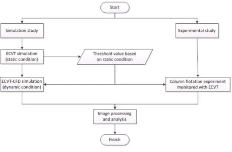
Fig. 1. Flow chart of the study.
2.1. Sensor Design and Sensitivity
32-electrode ECVT sensors (8-electrode per plane) were used both in simulation and experiment (Fig. 2). Diameter and height of ECVT sensor are 50 mm and 100 mm respectively. The shape of the electrode is rectangular with the dimension of 17 mm x 17 mm. The use of shifted plane design of ECVT sensor
between each electrode’s plane is based on [19]. The number of measurement produced using 32-electrode
is based on the Eq. (1):
(1)
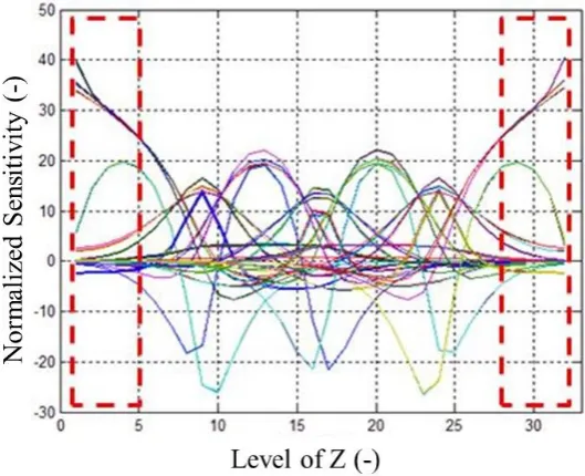
Thus, we got the measurement data of 496, where N is 32. The measurement data also represents the electric field of each pair of electrodes. The distribution of electric field in the sensor can also be used for identifying sensing zone and dead zone as shown in Fig. 3. Sensing zone or sensitive zone is an area where the objects can be easily detected whilst the dead zone is an area where the objects cannot be easily detected due to no variations of its electric field. Figure 3 shows the corelation graph between normalized sensitivity for all 496 capacitance pairs and the axial direction (z-axis) of the sensor. The dead zones are found at the bottom and the top portions of the sensor domain, which are the layer 1 to 5 and 26 to 32, respectively.
2 / ) 1
(
N N
[image:3.595.68.529.200.501.2]Fig. 2. 32-electrode ECVT sensor with 8-electrode per plane.
By adding more variation in the simulation, the distribution curve would be smoother, hence the good convergence shape image would be achieved [19].
Fig. 3. Axial distribution of normalized sensitivity for all 496 capacitance pairs. The dead zones are indicated by the dashed line.
2.2. ECVT Simulation of Bubbles Swarm model (Static Condition)
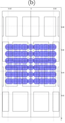
[image:4.595.197.420.85.281.2] [image:4.595.163.428.371.586.2](a)
(b)
Fig. 4. The object of simulation - a bubble swarm model. (a) top-view. (b) side-view.
2.3. ECVT-CFD Simulation
ECVT-CFD simulation is a combination of CFD and ECVT simulation. As the first step, CFD simulation was conducted to obtain the flow structures, and after that ECVT simulation was carried out by governing the electrical properties of phases previously generated by CFD simulation. Two-phase system approach has been used in the CFD simulation, where gas bubbles regarded as gas phase, and pulp (a mixture of ore, reagents, and water) as a liquid phase. Density and viscosity parameters of gas and liquid phase were
adjusted based on the real condition of column flotation experiment, which is 1 kg/m3 and 1 x 10⁻⁶
Pascal/m2 for gas phase, and 1,280 kg/m3 and 1.83 x 10⁻⁶ Pascal/m2 for the liquid phase. The diameter and
height of CFD simulation were set to 50 mm and 45 mm. Boundaries of CFD simulation were defined as
wall, inlet, and outlet. Hence, the flotation column’s wall was considered as a wall, the bottom of the
column was set as an inlet, and top of the column was assumed as the outlet (see Fig. 5). The wall and outlet boundaries were in a zero gradient condition which means constant. Inlet (bottom of the column) was varied to define the gas injection variation which was set for each CFD simulation to a fixed value (0.02, 0.03, and 0.04 m/s). To obtain the results of CFD simulation as a function of gas injection, the OpenFOAM was used for solving the Navier-Stokes equation which can be seen in Eq. (2).
𝜕𝛼
𝜕𝑡+ (𝑈∇)𝛼 = 0 (2)
Where 𝛼 is the volume fraction which was set as 0 (zero) for gas phase and 1 (one) for the liquid phase. In
which, density and kinetic viscosity of 𝛼 were expressed as the following Eq. (3) and Eq. (4):
𝜌(𝑋, 𝑡) = 𝜌𝑤𝑎𝑡𝑒𝑟𝛼 + 𝜌𝑎𝑖𝑟(1 − 𝛼)
(3)
𝜇(𝑋, 𝑡) = 𝜇𝑤𝑎𝑡𝑒𝑟𝛼 + 𝜇𝑎𝑖𝑟(1 − 𝛼) (4)
CFD simulation results were then used as the objects with permittivity in ECVT simulation. The 𝛼 values,
which were the flow structures from CFD simulation, were converted to electrical properties as relative
permittivity through python program. In the ECVT simulation, the relative permittivity of bubbles where 𝛼
equalled to 0 was 1, while the pulp where 𝛼 equalled to 1 was 12. The input voltage of each electrode was
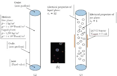
[image:5.595.352.464.95.306.2]Fig. 5. Boundary conditions of ECVT-CFD. (a) CFD simulation, (b) example of flow structure result, (c) ECVT simulation.
2.4. Global Thresholding
Segmentation involves separating a raw image into regions that correspond to the objects. Thresholding is one of the simpler segmentation methods. Here in the study, global thresholding method was used to distinguish the liquid phase and the gas phase. The common method of global thresholding as in Eq. (5):
𝑔(𝑥, 𝑦, 𝑧) = {
0, 𝑓(𝑥, 𝑦, 𝑧) < 𝑇
1, 𝑓(𝑥, 𝑦, 𝑧) ≥ 𝑇
(5)
where T is the thresholding value, 𝑓(𝑥, 𝑦, 𝑧) is the 3-D image before thresholding and 𝑔(𝑥, 𝑦, 𝑧) is the 3-D
image after thresholding. In this study, to get the optimum T, we compare the result of thresholding process to the phantom image from simulation data. Otherwise, T values obtained were averaged and used for thresholding on the ECVT-CFD simulation and experiment images results.
2.5. Relative Accuracy Measurement
Error percentage measures the accuracy of a measurement by comparing a tested value with an accepted value. The error was calculated in the following Eq. (6):
𝑒𝑟𝑟𝑜𝑟 (%) =
|𝐸−𝐴|𝐴
𝑥100%
(6)
where E is a tested value and A is an accepted value. In this study, simulation results are the tested value, while the experimental results are the accepted value. If the error between simulation and experimental results is less than expected, then the CFD codes are good, otherwise poor. Thus, relative accuracy (a in %) of the simulation results compared with the experimental results can be expressed as follow:
[image:6.595.108.491.81.331.2]2.6. Column Flotation Experiment with ECVT System
The experiment was conducted using a column with 50 mm diameter and 150 mm total height, as shown in Fig. 6. An air sparger made from ceramic material was installed at the bottom of the column. ECVT sensors as described previously were set at 5 cm above the sparger. The gas injection variation was set at the same value of CFD simulation, which is 5% solid-water. Feed, mixture reagents which were conditioned for 15 minutes prior the usage, was injected from the top of the column so that the separation occurred. On the other side, ECVT system captured the data signal of flow phenomena and transferred it to a computer for further analysis.
Fig. 6. Schematic diagram of column flotation experiment monitored by ECVT system [20].
3.
Results and Discussion
All 3-D ECVT reconstructed images were reconstructed using Iterative Linear Back Projection (ILBP) algorithm technique. Since the quality of reconstructed image using ILBP algorithm depends on the
constant 𝛼 (gain factor) and a number of iteration, thus to obtain the optimum parameters, those two
parameters were varied on the reconstruction process and evaluated by using correlation coefficient (CC)
value comparing phantom and reconstructed images. In this study, 𝛼 and iteration were limited to 0.1-1
with interval 0.1 and 100 with interval 1, respectively. The simulation was set as in static simulation (1 layer) as seen in Fig. 8(a). The detail about the algorithm technique can be found in [21].
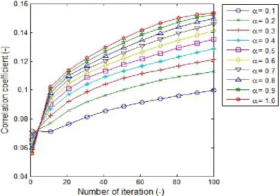
Figure 7 shows the relation between the CC and number of iteration with 𝛼 from 0.1to 1 on ILBP
system. Based on this study, the optimum parameters for 𝛼 and iteration are 1 and 100, respectively. Thus,
[image:7.595.85.497.203.531.2]Fig. 7. Relationship between correlation coefficient and iteration with 𝛼 0.1-1 on ILBP system.
3.1. ECVT Simulation of a Bubble Swarm Model (Static Condition)
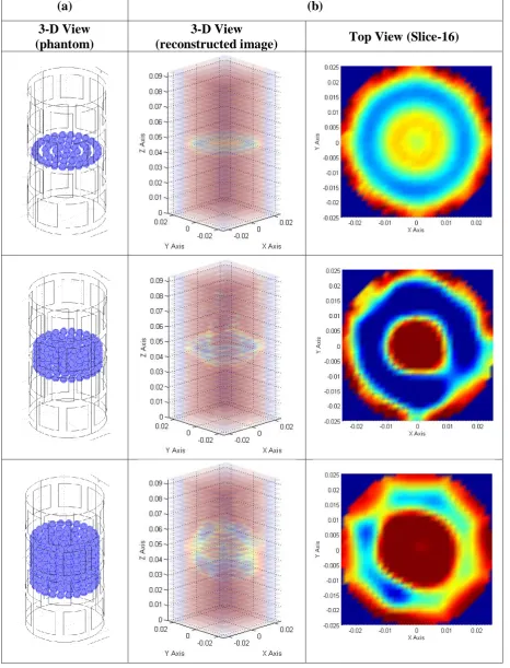
Figure 8 shows the three-dimensional reconstructed images compared with the phantom of the static condition. Figure 8(a) is the real object of simulated phantom and Fig. 8(b) is the reconstructed images of ECVT seen in 3-D and axial views at slice 16. The result showed that the simulated objects as bubble swarm model of 1, 3, and 6 layer(s) were significantly different qualitatively (Fig. 8). Idealy, as can be seen in Fig. 8, red color depicts the liquid phase, while blue color depicts the gas phase. Due to the ill-posed and ill-conditioned characteristics of ECVT method, the reconstructed images will have some errors. Also measurement and numerical reconstructed image, as well as the algorithm technique, contributes the errors. As seen in Fig. 8(b), the center region of each reconstructed image is dominated with the high permittivity values (yellow-red colors), whilst air-bubble is distributed homogeneously in phantom object (Fig. 8(a)). Thus, the thresholding method is needed to quantify each fraction (liquid and gas phases) as describe in previous section. Threshold value was determined by estimating the fraction volume of each phase based on the permittivity distribution compared to the phantom. Based on the simulation, the threshold values for each simulation are 0.380, 0.410, and 0.503 for 1, 3, and 6 layer(s) simulation, respectively. Thus, the average T value of 0.431 was used for all ECVT-CFD simulations and ECVT experiments in the current work, where the permittivity values higher and equal than T value were defined as a liquid phase while otherwise they are defined as gas (bubbles) phase.
3.2. Bubbles Imaging
[image:8.595.85.493.111.396.2]which, the values lower than T are defined as gas phase, and the values higher and equal than T are defined as liquid phase.
(a)
(b)
3-D View
(phantom)
3-D View
(reconstructed image)
Top View (Slice-16)
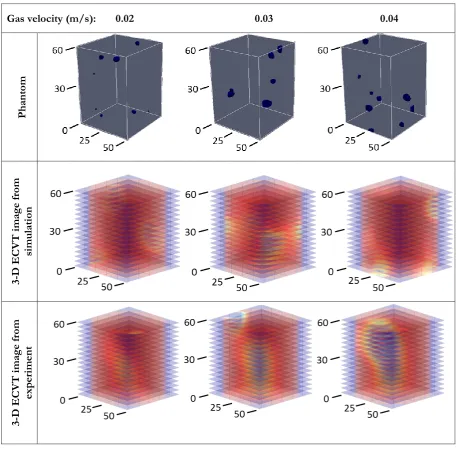
[image:9.595.67.534.119.731.2]As shown in Fig. 9, the number of bubbles generated independently was affected by the gas injection. Qualitatively, the reconstructed images from simulation and experimental results were visible similar. However it seems that the reconstructed images of bubbles visualize a bubble swarm rather than individual bubble. At low gas velocity (0.02 m/s), the shapes of bubbles imaging were blurred in both of simulations and experimental imaging results. At higher gas velocity 0.03 and 0.04 m/s, the bubbles shapes became clearer. The shapes of bubbles indicated the movement from the bottom part to the top of the z axis. In general, the increase of gas injection could increase a number of bubbles and also affected the results of 3-D ECVT reconstructed images. Bubbles agglomeration phenomena were also observed in both, simulation and experimental results.
Gas velocity (m/s): 0.02 0.03 0.04
P ha nt om 3-D EC V T im ag e fro m si m ul at io n 3-D EC V T im ag e fro m ex pe ri m en t
Fig. 9. The comparisons of ECVT-CFD simulation and ECVT experiment with the phantom from CFD simulation (units in mm).
[image:10.595.69.526.212.662.2]column flotation experiment, the bubble motion and bubble rise velocity were influenced by gas injection which was blown by compressor [22, 23]. In general when gas injection increased, the bubble moved
spirally and the shape of the rising bubble could be sphere or oval [24–26]. At this stage, those
phenomenon were also observed, however more detail investigation may be conducted to elucidate the bubbles or bubble swarm movements. To quantify and compare the bubble fraction of each study (simulation and experiment), the average threshold value of 0.431 obtained in section 3.1 was used. The volume elements (voxels) [19] less than threshold value were defined as gas phase while the higher voxels were defined as a liquid phase for both ECVT-CFD simulation and ECVT experimental studies.
3.3. Bubble Fraction and Relative Accuracy
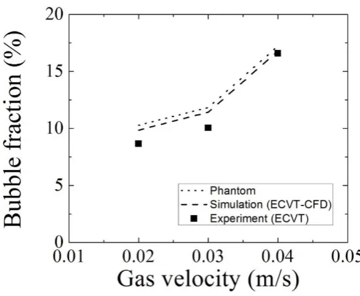
Figure 10 shows a relation between bubble fraction and gas injection or gas velocities. Generally, the bubble fraction increased when gas injection or gas velocity is increased. For phantom (CFD results), the bubble fraction increases from 10.3% to 17.2%, whilst for simulation study (ECVT-CFD results), the bubble fraction increased from 9.85% to 16.8%, and for experimental study (ECVT results), the bubble fraction increased from 8.64% to 16.6%.
The differences of bubble fraction percentage between simulation and experiment showed in Fig. 10 may be caused by the differences in some parameters which are not governed in detail by CFD simulation. For example, density and viscosity of the simulation are calculated based on the number of theory, while the density and viscosity of experimental conditions are calculated based on actual weight and volume of the component substances, which included the reagents itself, some water and galena inside. Hence, simulated conditions for pulp might differ with the experimental conditions. Another reason is surface tension. In the OpenFOAM simulation, the surface tension between bubble-pulp used the maximum limit of the sigma value, consequently, the bubbles generated were not easily broken, while in the experiment most of the bubbles will always be ruptured and it affected the results.
As for column pressure, in the simulation, column pressure used zero gradient condition, which means the pressure generated will be distributed evenly on the column; therefore the pressure on the entire surface of the column has the same value. In the experimental conditions, column pressure was not uniform. The pressure at the centre of the column was higher than at the edge, and also from the bottom to the top of the column. These might cause bubble fraction discrepancies between simulation and experiment.
Table 1 shows relative accuracy of ECVT-CFD simulation compared with the ECVT experiment. Basically, the relative accuracy of simulations and experimental results were more than 86%. At the higher gas velocity of 0.04 m/s, the relative accuracy increased up to 98.7 %. This indicated a relatively good correlation between simulations and experiments. However, further improvement in optimum accuracy is still needed.
4.
Conclusion and Future Direction
Fig. 10. The relationship between bubble fraction and velocity of gas obtained from simulation and experimental results.
Table 1. Relative accuracy of ECVT-CFD simulation compared with ECVT experiment.
Gas velocity (m/s) Relative accuracy (%)
0.02 86.0
0.03 86.3
0.04 98.7
Acknowledgements
Acknowledgement from the authors to Research Grant with the contract
002/SP2H/LT/DRPM/IV/2017
from Directorate of Research and Community Engagement Ministry ofResearch, Technology and Higher Education of Republic of Indonesia. Equipment supports of data acquisition system, and computation facility from C-Tech Laboratory is gratefully appreciated.
References
[1] M. S. Oliveira, R. C. Santana, C. H. Ata??de, and M. A. S. Barrozo, “Recovery of apatite from flotation tailings,” Sep. Purif. Technol., vol. 79, no. 1, pp. 79–84, 2011.
[2] P. N. Holtham and K. K. Nguyen, “On-line analysis of froth surface in coal and mineral flotation
using JKFrothCam,” Int. J. Miner. Process., vol. 64, no. 2–3, pp. 163–180, 2002.
[3] J. Kaartinen, J. Hätönen, H. Hyötyniemi, and J. Miettunen, “Machine-vision-based control of zinc
flotation—A case study,” Control Eng. Pract., vol. 14, no. 12, pp. 1455–1466, 2006.
[4] C. Aldrich, C. Marais, B. J. Shean, and J. J. Cilliers, “Online monitoring and control of froth flotation systems with machine vision: A review,”Int. J. Miner. Process., vol. 96, no. 1–4, pp. 1–13, 2010.
[5] A. Jahedsaravani, M. H. Marhaban, and M. Massinaei, “Prediction of the metallurgical performances of a batch flotation system by image analysis and neural networks,” Miner. Eng., vol. 69, pp. 137–145, 2014.
[6] I. Jovanović, I. Miljanović, and T. Jovanović, “Soft computing-based modeling of flotation
processes—A review,” Miner. Eng., vol. 84, pp. 34–63, 2015.
[7] G. Bonifazi, S. Serranti, F. Volpe, and R. Zuco, “Characteristisation of flotation froth colour and
[image:12.595.143.454.387.439.2][8] A. Mehrabi, N. Mehrshad, and M. Massinaei, “Machine vision based monitoring of an industrial flotation cell in an iron flotation plant,” Int. J. Miner. Process., vol. 133, pp. 60–66, 2014.
[9] F. Wang, Q. Marashdeh, L.-S. Fan, and W. Warsito, “Electrical Capacitance Volume Tomography:
Design and Applications,” Sensors, vol. 10, no. 3, pp. 1890–1917, 2010.
[10] J. M. Weber, K. J. Layfield, D. T. Van Essendelft, and J. S. Mei, “Fluid bed characterization using
electrical capacitance volume tomography (ECVT), compared to CPFD software’s barracuda,” Powder Technol., vol. 250, pp. 138–146, 2013.
[11] A. Wang, Q. Marashdeh, and L. S. Fan, “ECVT imaging and model analysis of the liquid distribution
inside a horizontally installed passive cyclonic gas-liquid separator,” Chem. Eng. Sci., vol. 141, pp. 231–
239, 2016.
[12] J. M. Weber and J. S. Mei, “Bubbling fluidized bed characterization using electrical capacitance volume
tomography (ECVT),” Powder Technol., vol. 242, pp. 40–50, 2013.
[13] A. Wang, Q. Marashdeh, B. J. Motil, and L. S. Fan, “Electrical capacitance volume tomography for
imaging of pulsating flows in a trickle bed,” Chem. Eng. Sci., vol. 119, pp. 77–87, 2014.
[14] F. Wang, Z. Yu, Q. Marashdeh, and L. S. Fan, “Horizontal gas and gas/solid jet penetration in a gas
-solid fluidized bed,” Chem. Eng. Sci., vol. 65, no. 11, pp. 3394–3408, 2010.
[15] C. Pradeep, R. Yan, S. Vestøl, M. C. Melaaen, and S. Mylvaganam, “Electrical capacitance tomography
(ECT) and gamma radiation meter for comparison with and validation and tuning of CFD modeling
of multiphase flow,” in IST 2012 - 2012 IEEE International Conference on Imaging Systems and Techniques, Proceedings, 2012, pp. 45–50.
[16] H. G. Wang, W. Q. Yang, P. Senior, R. S. Raghavan, and S. R. Duncan, “Investigation of batch
fluidized-bed drying by mathematical modeling, CFD simulation and ECT measurement,” AIChE J.,
vol. 54, no. 2, pp. 427–444, 2008.
[17] Y. Zhang, E. W. C. Lim, and C. H. Wang, “Pneumatic transport of granular materials in an inclined
conveying pipe: Comparison of computational fluid dynamics-discrete element method (CFD-DEM),
electrical capacitance tomography (ECT), and particle image velocimetry (PIV) results,” Ind. Eng. Chem.
Res., vol. 46, no. 19, pp. 6066–6083, 2007.
[18] A. Uribe-Salas, R. Perez-Garibay, and F. Nava-Alonso, “Operating parameters that affect the carrying
capacity of column flotation of a zinc sulfide mineral,” Miner. Eng., vol. 20, no. 7, pp. 710–715, 2007.
[19] W. Warsito, Q. Marashdeh, and L.-S. Fan, “Electrical capacitance volume tomography,” IEEE Sens. J.,
vol. 7, no. 4, pp. 525–535, Apr. 2007.
[20] D. Haryono, S. Harjanto, H. Nugraha, M. Al Huda, and W. P. Taruno, “Column flotation monitoring
based on electrical capacitance volume tomography: A preliminary study,” AIP Conf. Proc., vol. 1805, no. 1, p. 50005, 2017.
[21] W. Q. Yang, D. M. Spink, T. a York, and H. McCann, “An image-reconstruction algorithm based on
Landweber’s iteration method for electrical-capacitance tomography,” Meas. Sci. Technol., vol. 10, no.
11, pp. 1065–1069, 1999.
[22] A. A. Kulkarni and J. B. Joshi, “Bubble formation and bubble rise velocity in gas-liquid systems: A
review,” Ind. Eng. Chem. Res., vol. 44, pp. 5873–5931, 2005.
[23] W. Kracht and J. A. Finch, “Effect of frother on initial bubble shape and velocity,” Int. J. Miner.
Process., vol. 94, no. 3–4, pp. 115–120, 2010.
[24] Y. H. Tan and J. A. Finch, “Frother structure-property relationship: Effect of alkyl chain length in
alcohols and polyglycol ethers on bubble rise velocity,” Miner. Eng., vol. 95, pp. 14–20, 2016.
[25] J. Jamaludin, R. A. Rahim, H. A. Rahim, M. H. Fazalul Rahiman, S. Z. Mohd Muji, and J. M. Rohani,
“Charge coupled device based on optical tomography system in detecting air bubbles in crystal clear water,” Flow Meas. Instrum., vol. 50, pp. 13–25, 2016.
[26] S. A. Hussain and A. Idris, “Spiral motion of air bubbles in multiphase mixing for wastewater
![Fig. 6. Schematic diagram of column flotation experiment monitored by ECVT system [20]](https://thumb-us.123doks.com/thumbv2/123dok_us/8107408.235458/7.595.85.497.203.531/fig-schematic-diagram-column-flotation-experiment-monitored-ecvt.webp)