Non-linear principal component analysis (approximation by a second-order Taylor series)

Rochester Institute of Technology

RIT Scholar Works

Theses

Thesis/Dissertation Collections

11-1-1984

Non-linear principal component analysis

(approximation by a second-order Taylor series)

John Viggiano

Follow this and additional works at:

http://scholarworks.rit.edu/theses

This Thesis is brought to you for free and open access by the Thesis/Dissertation Collections at RIT Scholar Works. It has been accepted for inclusion

in Theses by an authorized administrator of RIT Scholar Works. For more information, please contact

[email protected]

.

Recommended Citation

NON-LINEAR

PRINCIPAL

COMPONENT ANALYSIS

Approximation

by

a

Second-Order Taylor

Series

by

John

Anthony

Stephen Viggiano

A

thesis

submitted

in

partial

fulfillment

of

the

requirements

for

the

degree

of

Master

of

Science

in

Statistics

at

the

Center

for

Quality

and

Applied

Statistics

of

the

College

of

Continuing

Education

of

the

Rochester

Institute

of

Technology

November,

1984

Thesis Advisor:

Professor

Nicholas

Zaino

NON-LINEAR PRINCIPAL COMPONENT ANALYSIS

(APPROXIMATION BY A SECOND ORDER TAYLOR SERIES)

I, JOHN ANTHONY STEPHEN VIGGIANO, grant permission to

the Wallace Memorial Library of Rochester Institute of

Technology, to reproduce my thesis in whole or in part.

Any reproduction will not be for commercial use or

profit.

John Anthony Stephen viggiano

profit.

G^

b^

ACKNOWLEDGEMENTS

The

author received

the

help

of many people

in

the

preparation of

this

thesis.

Many

individuals

come

to mind,

and

I

would

like

to

thank

them

for

their

assistance.

In

particular:

Mrs Lynn Tessar

of

the

Ridgewood, NJ,

Library,

for

her

assistance

in

locating

the

authorities cited

herein.

The

author

naturally

assumes all responsibility

for

any

inaccuracies

and omissions

that

there

may

be;

Dr Austin

Bonis,

late

chairman of graduate statistics at

RIT,

for

his

initial

encouragement and assistance;

The

authors

family

and

friends,

some of whom

I

might

have

depended

on a

little

too

much,

and

to

some of whom

I

may

have

been

perhaps a

little

more eccentric

than

usual;

and;

Professor Nicholas

Zaino,

the

author's advisor, who was

very

tolerant

of

the

author's

idiosyncrasies,

and worked

hard

at

achieving

a

high

level

of rapport

throughout

the

duration

of

this

project.

DEDICATION

This

thesis

is dedicated

to

the

family

and

friends

of

the

author's,

for

EPIGRttl

Look

around,

my

little

friend:

Jubilation

in

the

land

When

Johnny

strikes

up

the

band

-Warren

Zevon

When

it

hits

you,

you'll

holla

"Yes,

indeed!"

ABSTRACT

Linear

Principal

Component

Analysis

(LPCA)

has been

applied

in

multi variate analysis

because

of

i ts

many

optimality properties.

However,

when applied

to

locate

singularities

in

a set of

data,

LPCA

is

only

able

to

locate

linear

singularities.

If

the

problem

being

considered

tends

to

produce variables wi

th

non-linear

relationships,

such as with non-linear

regression,

LPCA

is

necessarily

of

limited

utility

in

identifying

singularities.

Non-linear

generalizations of

PCA have

been

suggested

in

the

literature.

Essentially,

these

involve

augmenting

the

data

with

higher-order

terms,

in

particular square and cross product

terms,

and

running

a

LPCA

on

the

augmented

data

set.

The

problem with

this

approach

is

that

the

fundamental

property of parsimony

is

violated

because

the

number of principal components

is

greater

than

the

number of original variates.

Further,

the

dimensionality

of

the

augmented

data

set

increases

quadrat

ical

ly

with respect

to

the

number of original variates.

This

greatly

increases

the

computational

load for

practical-sized problems.

A

new method

is

proposed

in

this

thesis.

It

involves writing the

general non-linear model as a

Taylor

Series

and

truncating

after

the

second-order

terms.

The

data

are centered about

their means,

and

the

square and cross-product values are computed.

The

covariance matrix

for

the

augmented problem

is

computed.

The

non-linear singularities

(or

near singularities) are obtained

by

running

a canonical regression

using

the

'original*

and "added* sets as partitions.

The

advantage

here

is

that

no more principal components

may

be

extracted

here

than

there

are variates

in

the

original

data

set,

so

the

principle of

parsimony

is

upheld.

TABLE

OF CONTENTS

Chapter

One

-Introduction

...

1

Purpose

1

Scope

1

History

and

Background

1

Non-Linear

Principal

Component

Analysis

2

A New Approach

5

Other

Approaches

6

Chapter Two

-

A Model

for Non-Linear

Principal

Components

7

The Model

for

Linear

Principal

Components

7

A Model

for Non-Linear

Principal

Components

. .

7

The Taylor

Series for

One Variable

8

The Taylor

Series for

Several

Variables

8

A

Practical

Model

for Non-Linear

Principal

Component Analysis.

8

Chapter Three

-

Determination

of

the

Coefficients

10

Canonical

Regression

10

Problems

with

the

Canonical

Correlation

Approach

11

Square Terms have

high

correlation with

corresponding

1 inear

terms

11

The

number of "added" variables

becomes

too

large

12

A

singularity

in

either partition stops

the

process

12

General

Procedure

for Non-Linear

Principal

Component Analysis.

. .

14

Chapter

Four

-Experimental

Method

15

Chapter

Five

-Experimental

Results

17

Gnanadesikan/Wi Ik

Problem

17

Non-Linear

Regression

Example

19

Vectors

in

the

null space of

B

24

Chapter

Six

-Summary

26

Conclusions

and

Recommendations

26

Recommendations

26

Suggestions for

Further

Investigation

27

Notes

29

LIST OF

TABLES

Table

1.

Data from

2-variate

Gnanadesikan-Wi Ik

Example

3

Table

2.

Covariance

Matrix

from Gnanadesikan-Wi Ik

Example.

...

4

Table

3.

Eigenanalysis

for

Gnanadesikan-Wi Ik

Example

4

Table

4.

Dimensionality

of

the Augmented Data Set

5

Table 5.

Orthogonal

Polynomials

12

Table

6.

Dimensionality

of

Matrices for

Old

and

New Methods

13

Table

7.

Rotation

for

Gnanadesikan/Wi Ik

Problem

16

Table

8.

Matrices

A

and

B for

Gnanadesikan/Wi Ik

Problem

16

Table

9.

Non-Linear

Principal

Component Analysis

of

Gnandesikan/Wilk

Problem

18

Table

10.

Data

for

2-parameter Non-Linear

Regression

Problem

19

Table

11.

Covariance Matrix

for Non-Linear

Regression

Problem

20

Table

12.

Rotation

for Non-Linear

Regression

Problem

21

Table

13.

Matrices A

and

B for Non-Linear

Regression

Problem

21

Table

14.

Non-Linear

Principal

Component Analysis

of

Non-Linear

Regression

Problem

23

Table

IS.

Least

Significant Principal

Components

and

Vectors

in

the Null

Space

of

B

25

LIST

OF

FIGURES

Figure

1.

First Non-Linear

Principal

Component

24

COPTER

ONE

INTRODUCTION

PURPOSE

The

purpose of

this

thesis

will

be

to discuss

a generalization of

the

Principal

Component

model

to

the

non-linear case.

This

particular gen

eralization

differs

from

the

one previously presented

in

the

literature

in

that

the

new method produces

the

same number

<rather

than

more) of

principal components as

there

are variates.

SCOPE

This

thesis

will

discuss

a generalization of

Linear

Principal

Component

Analysis

(LPCA)

to

a non-linear model.

For

expediency,

a

Taylor

series

expansion will

be

used.

This

thesis

will

be

limited

to

discussion

of models with

truncation

after no

higher

than

the

second-order

terms.

Methods

for

the

computation of

the

coefficients will

be

discussed.

One

of

these,

Canonical

Regression,

will

be

examined

in

some

detail,

inclu

ding

numerical examples.

Another method,

Maximum

Likelihood,

will

be

discussed

in

less detail.

The

conclusions and recommendations of

the

author,

as well as suggestions

for

further

research,

will

be

presented.

HISTORY

AND

BACKGROUND

In

a

1901

paper entitled

"On

Lines

and

Planes

of

Closest

Fit.

.

CU

Karl

Pearson

spawned a

branch

of statistics

that

is

purely multivariate

that

is,

having

no univariate analog.

This

paper was precursor

to

work

by

Hotelling, Thurstone,

et

alii,

in

what

has

generally

become

known

as

Principal

Component

Analysis.

Pearson's

1901

paper

discussed

an alternative

for

ordinary

least

squares.

Ordinary

least

squares

(ala

Gauss

and

Legendre)

pre-supposes

that

any

error

is

strictly contained

in

the

response

variable;

the

predictor variable

being

error-free.

With

correlation

data,

however,

with

both

predictor and response variables

coming from

a common

bi-variate

distri

bution,

this

assumption

is

violated

there

is

no

longer

a clear

dis

tinction

between

independent

and

dependent

variables.

Linear

Principal

Component

Analysis

(LPCA)

is

useful when several corre

lated

variables are under

investigation.

Some

of

its

applications

1.

Variate

Peduction

through

parsimony

of

description

2.

Transformation

to

a set of uncorrelated

variates

(spher

ic i

zat

i

on)

3.

Identification

of

linear

singularities

(or

near singularities)

4.

Orthogonal

Regression

While

the

first

pair are of general application,

the

second pair are

useful only when an

underlying

relationship

between

and amongst

the

variates

(i.e.,

singularity)

is

linear

(or

nearly so).

When

this

is

not

the

case,

LPCA

is

necessarily of

limited

value.

When

a

non-1

i

near singul ar

i

ty exists,

LPCA

will

be

unable

to

locate

it.

This

problem

becomes

more

important

as

the

number of variates

becomes

large.

Gnanadesikan

and

Wilk

give an example

in

3

variates which, while

being

perfectly

related

(on

a paraboloid

in

3-space)

do

not appear

to

have

any

interrelationship

when plotted pairwise.

C3]

Practically

speaking,

this

situation will arise

in

Non-linear

Regression

Analysis,

where

the

parameter estimates will

have

non-linear relations

both

to

the

response and

among

themselves.

This

may

be

extended

to

the

partial

derivatives

of

the

model

from

which

the

increments

for

the

parameter estimates are

determined.

It

seems worth

pointing

out

that

while

for

linear

regression

the

linear

relationships are of _primary

interest,

in

non-linear regression

the

non-linear relationships are

nec-essarilly of consequence.

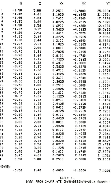
NON-LINEAR

PCA-

Gnanadesikan

and

Wilk

proposed an extension of

the

LPCA

techniaue

to

include

also

the

case of singularities

in

the

data

contain

ing

second-order

terms.

C41

They

included

an

example,

with

the

under

lying

relationship

Y

=

2

+

4X

?

4XX,

which

is

presented

here

in

Tables

1-3.

Essentially,

this

method

involved

augmenting

the

original

data

set with

all second-order

terms

(squares

and cross-products of

the

original vari ates) and

performing

a

LPCA

on

the

augmented

data

set.

This

is

similar

to

techniques

recommended

by

others

(e.g.,

Roderick

McDonald,

"A

general

XX

XY

YY

1

-1.50

5.00

2.2500

-7.5000

25.0000

2

-1.45

4.61

2.1025

-6.6845

21.2521

3

-1.40

4.24

1.9600

-5.9360

17.9776

4

-1.35

3.89

1.8225

-5.2515

15.1321

5

-1.30

3.56

1.6900

-4.6280

12.6736

6

-1.25

3.25

1.5625

-4.0625

10.5625

7

-1.20

2.96

1.4400

-3.5520

8.7616

8

-1.15

2.69

1.3225

-3.0935

7.2361

9

-1.10

2.44

1.2100

-2.6840

5.9536

10

-1.05

2.21

1.1025

-2.3205

4.8841

11

-1.00

2.00

1.0000

-2.0000

4.0000

12

-0.95

1.81

0.9025

-1.7195

3.2761

13

-0.90

1.64

0.8100

-1.4760

2.6896

14

-0.85

1.49

0.7225

-1.2665

2.2201

15

-0.80

1.36

0.6400

-1.0880

1.8496

16

-0.75

1.25

0.5625

-0.9375

1.5625

17

-0.70

1.16

0.4900

-0.8120

1.3456

18

-0.65

1.09

0.4225

-0.7085

1.1881

19

-0.60

1.04

0.3600

-0.6240

1.0816

20

-0.55

1.01

0.3025

-0.5555

1.0201

21

-0.50

1.00

0.2500

-0.5000

1.0000

22

-0.45

1.01

0.2025

-0.4545

1.0201

23

-0.40

1.04

0.1600

-0.4160

1.0816

24

-0.35

1.09

0.1225

-0.3815

1.1881

25

-0.30

1.16

0.0900

-0.3480

1.3456

26

-0.25

1.25

0.0625

-0.3125

1.5625

27

-0.20

1.36

0.0400

-0.2720

1.8496

28

-0.15

1.49

0.0225

-0.2235

2.2201

29

-0.10

1.64

0.0100

-0.1640

2.6896

30

-0.05

1.31

0.0025

-0.0905

3.2761

31

0.00

2.00

0.0000

0.0000

4.0000

32

0.05

2.21

0.0025

0.1105

4.8841

33

0.10

2.44

0.0100

0.2440

5.9536

34

0.15

2.69

0.0225

0.4035

7.2361

35

0.20

2.96

0.0400

0.5920

8.7616

36

0.25

3.25

0.0625

0.8125

10.5625

37

0.30

3.56

0.0900

1.0680

12.6736

38

0.35

3.89

0.1225

1.3615

15.1321

39

0.40

4.24

0.1600

1.6960

17.9776

40

0.45

4.61

0.2025

2.0745

21.2521

41

0.50

5.00

0.2500

2.5000

25.0000

MEAN

S:

-0.50

2.40

0.6000

-1.2000

7.3252

TABLE

1.

[image:12.533.58.415.71.657.2]

X

Y

XX

XY

YY

14.3500

-5.6E-09 -14.3500

50.4833

7.5E-09

64.1732

16.0433

-32.0866

358.912

[image:13.533.95.428.70.194.2]

18.3608

-58.5050

210.888

89.7279

-179.456

2080.26

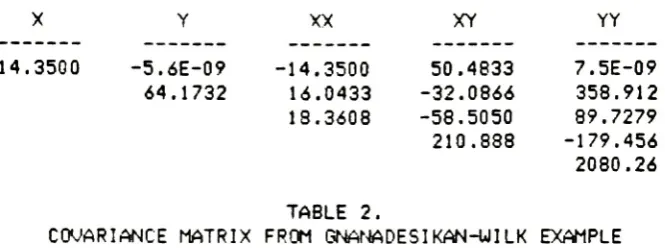
TABLE 2.

COVARIANCE

MATRIX

FROM GNANADESIKAN-WILK EX^IPLE

(Note:

Gnanadesikan

and

Wilk

used

the

sum-of-squares

matrix,

rather

than

the

covariance matrix.

The

covariance matrix may

be

obtained

by

multi

plying

the

sum-of-squares matrix

by

the

reciprocal of

the

number of

degrees

of

freedom.

In

order

to

permit more

direct

comparison,

the

sum-of-squares matrix will

be

used rather

than

the

covariance matrix

in

this

thesis.)

2163.63

219.915

EIGENVALUES

2.258

2.223

0.000009

EIGENVECTORS

-0.002513

0.169321

0.

0

44843

-0.094253

0.980015

0.246077

0.011882

-0.243106

0.932909

0.099425

0.508757

0.758811

0.319056

-0.212548 -0.135640 -0.442445

0.604229

0.593499

0.274991

-0.106239

0.696310

-0.174076

0.696311

0.0000004

0.0000003

TABLE

3.

EIGENANALYSIS

FOR

GNANADESIKAN-WILK

EXAMPLE.

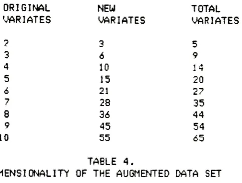
In

a p-variate

problem,

there

will

be

p(p-D/2 cross products and

p

squared

terms,

augmenting

the

original

data

set

by

p(p*l)/2 variates

to

p(p+3)/2 variates.

Table

4

contains

the

number of variates

in

the

aug

mented

data

set

for

p

=

2,3

10.

Note

that

the

_{number of variates}

in

the

augmented

data

set

increases

quadrat

ical

ly

with respect

to

the

number

of variates

in

the

original

data

set.

Immediately,

two

disadvantages

to

this

approach

become

apparent:

1)

As

the

number of

"original"

variates

approaches a size

for

which

PCA

might

be

considered,

the

number of variates

in

the

augmented

data

set

increases

with

quadrat

ic

rap idi

ty-2)

The

number of

resulting

principal

components will always

be

larger

than

the

[image:13.533.75.431.292.465.2]

The

first

of

these

problems

is

unattractive particularly

from

a practical

point of view.

Not

only

will vast amounts of computer storage

be

neces

sary,

but

the

matrices

involved

will

be

of so

high

an order

that

computa

tion

will

be

slowed

down

considerably.

ORIGINAL

NEW

TOTAL

VARIATES

VARIATES

VARIATES

2

3

5

3

6

9

4

10

14

5

15

20

6

21

27

7

28

35

8

36

44

9

45

54

[image:14.533.127.373.157.342.2]

10

55

65

TABLE 4.

DIMENSIONALITY

OF

THE AUGMENTED DATA SET

A

double

penalty

is

extracted as

the

price of

taking

this

approach,

for

not only

does

the

effort

involved

in

the

e

igenanalysis

increase

cubically with respect

to

the

total

number of

variates,

but

the

total

number of

variates

in

the

e

i

genanalysis

increases

quadrat

i

cal

1

y with respect

to

the

original number of variates.

This

yields an overall quintic effect.

The

second problem

is

objectionable

from

an

intuitive

point of view.

The

principle of parsimony

(which

Ted Jackson

describes

as

"the

name of

the

game"

in

PCA

[61)

mandates

that

fewer

(not

more!) principal components

be

used

than

the

original number of variates.

The

fact

that

for

all our

number

crunching

we obtain a

less

parsimonious

solution,

rather

than

a

more parsimonious

one,

makes

this

approach unattractive.

A

NEW

APPROACH-

If

it

is

_assumed

that

_what

is

_of

interest

is

the

_rela

tionships

between

and

among

the

variates,

Canonical

Correlation

may

be

used

to

studv

these

relationships.

Once

again,

the

data

matrix can

be

augmented

by

additional

terms

of

higher

order

(squares

and cross-products

for

a second-order

model),

and

the

covariance matrix computed.

A

canoni

cal correlation can

be

performed on

the

augmented

data

set,

putting

the

original variates

in

one

partition,

and

the

"added"

variates

in

the

other.

The

first

canonical correlation

function

would

indicate

the

best

linear

relationship

between

these

two

sets of variates.

This

approach

has

several advantages.

First,

recall

that

there

are no more canonical correlation

functions

as

there

are variates

in

either

partition.

Because

there

will

be

more variates

in

the

"added*

partition

than

in

the

original,

the

number of canonical correlation

functions

will

to

the

dimensionality

property

of

LPCA

(number

of principal components

does

not exceed

the

number of variates).

This

is

necessary

for

the

property

of parsimony.

Secondly,

the

function

of

interest

the

first

vector

to

be

extracted,

rather

than

the

last,

as with

the

Gnanadesikan-Wi Ik

approach.

The

advan

tages

to

this

include

faster

results and

improved

numerical accuracy.

In

addition,

the

matrices will

be

of more manageable

size,

both

physical

ly

(in

terms

of

dimension)

and algebraically

(in

terms

of rank).

For

example,

for

a

five

variate

problem,

a

5x5

matrix and a

15x15

matrix of

rank

5

will

be

analyzed, as opposed

to

a complete analysis of a

20x20

for

the

Gnanadesikan/Wi Ik

approach.

(A

scheme

for

further

reducing

the

size

of

the

larger

matrix,

say,

for

this

example,

to

a

8x8

or

9x9,

will

be

discussed.)

Five

vectors,

rather

than

20,

will complete

the

analysis.

OTHER

APPROACHES-

If

the

_problem

is

not so much

identification

of

the

relationships

among

the

variates,

but,

rather,

transforming

the

original variates

to

a new variate space

having

the

optimal

ity

properties of

Linear

Principal

Components,

another approach may

be

useful.

This

involves

the

maximization of a

likelihood function.

If

we stipulate

that

the

(as

yet undetermined) non-linear principal com

ponents come

from

a gaussian

population,

we could select

those

coeffi

cients

for

the

first NLPC

which maximize

the

liklihood

of

the

first

NLPCA

having

been

drawn

from

a gaussian

population;

the

second set would maxi mize

the

likelihood,

subject

to

orthogonality

restrictions,

etc.

Natu

rally,

no more principal components would

be

taken

than

we

have

variates.

However,

this

thesis

will

discuss

primarilly

the

first

approach

based

on

Canonical

Correlation.

This

choice was made

because

of software avail

ability,

rather

than

the

advantages and

disadvantages

inherent

to

both

CHAPTER TWO

A

MODEL

FOR NONLINEAR PRINCIPAL COMPONENTS

THE MODEL FOR LINEAR

PRINCIPAL

COMPONENTS-

The

adjective "linear*

derives

from

the

model

for

the

principal components

in

the

classic

(linear)

case:

where

zi

represents

the

i-th

linear

principal

component,

and

the

x's

represent

the

values of

the

original

(observed)

variates

from

a particu

lar

experimental unit.

This

model

is

as general as one can

hope

to

get

in

the

linear

case

-it

is

a

linear

combination of all

the

variates!

The

coefficients

vij

are usually selected

to

maximize

the

variance of z

for

a vector

v*

of unit euclidean

length.

(It

can

be

demonstrated

that

this

also maximizes

the

likelihood

of

z1,

having

been

drawn

from

a gauss

ian

population.)

Additionally,

the

restriction

that

a vector

v^_

must

be

orthogonal

to

all

preceeding

vectors

is

imposed.

The

simplest model

for

linear

principal components

is

also

the

most

general!

This

happy

fact

is

something

that

is

"bought"

by

imposing

the

restriction of

linearity

on

the

model.

As

a

result,

only one model need

be

considered

for

any given number of variates.

A MODEL FOR

NON-LINEAR

PRINCIPAL

COMPONENTS-Unfortunately,

there

are an

infinite

number of models

to

consider

for

the

non-linear case.

It

is

not

possible

to

empirically

build

a model

based

on

the

response as

is

done

in

non-linear

regression,

because

in

princpal component analysis

the

repsonse

is

not

known

until

the

end of

the

analysis!

Therefore,

some

general non-linear model

is

needed.

Some

species of general models one might consider are

those

of

the

infi

nite series genre.

These

include:

1.

Fourier

Series

2.

Asymptotic

Series

3.

Exponential

Series

4.

Taylor

Series

The

first

of

these

is

particularly suited

for

periodic

data.

The

second

precludes

inclusion

of

the

origin,

and may also provide poor resolution

far

from

the

origin.

The

last

two

are of more general

application,

with

the

latter

having

received

the

most attention

in

mathematical

literature.

The

properties of

the Taylor

Series

are well

known,

so

it

will

be

chosen

The

Taylor

Series

for

One Variable:

The

infinite Taylor

Series for

one

variable

is:

(2)

CO

j-o

where

the

coefficient

for

each

term

is:

(3)

a:

=

<&<*

)

The

Taylor

Series

for

Several

Variables-

The Taylor

Series

has

been

generalized

for

the

case of many variables.

This

involves

not only all

the

partial

derivatives

of

the

function,

but

also all

the

mixed partial

derivatives.

This

is

conveniently

written:

lM,A'^k)^)

with

the

powers of

the

partial

differential

operators

denoting

the

order of

the

derivative

of

the

function,

and products of partial

differential

operators

denoting

a mixture of partial

differentiation.

Once

the

coefficients

for

this

model are

obtained,

the

principal components may

be

computed,

and

then

they

may

be

modelled as

functions

of

the

original variates

desi

red.

for

a closed-form

non-1

i

near

as

solution,

if

A

Practical

Model

for

NLPCA-Obviously,

a model with an

infinite

number of

terms

is

entirely

impractical

for

use

in

a practical problem.

The

infinite series

is

usually

truncated

after a number of

terms

to

provide

an approximation.

Obviously,

the

more

terms

truncated

from

the

series,

the

cruder

the

degree

of approximation.

(This

rationale

is

used

by

people

to

justify

running

polynomial regressions with a

large

number of

terms. )

If

we

truncate

after

the

first

term,

ding

means,

we obtain

and se

t

the

^'s

to

the

corr

espon-(5)

1-1

'

which

is

the

model

for

linear

PCA.

are

retained,

the

model

becomes:

If

the

:6)

f,c)-

c^i^rN

**

c^k^rN^-f^^)

j1

j=f

fe--<

which

may

be

re-written:

(7)

fctt-

SK*-/)

+^(r-pOHi<*-/rV

where

^.is

the

gradient

vector,

and

H*.

is

the

Hessian

matrix,

of

the

i-th

principal component with respect

to

the

original

variates,

evaluated at

the

poi nt

7

=

jju

Naturally,

the

z's may

be

written as polynomials

in

the

x's.

In

the

case

of

(7),

it

should

be

remembered

that

this

form

(the

sum of a vector

dot

product and a quadratic

form)

is

equivalent

to

a second-order polynomial

in

the

x's,

containing

in

general all

the

square and cross-product

terms.

Because

the

simple polynomial

is

easier

to

work

with,

this

thesis

will

use

the

polynomial equivalent

to

(7),

with

the

understanding

that

this

polynomial

may

be

transformed

into

the

form

of

(7)

by

the

simple exercise

of

completing

squares.

Higher

order approximations are of course possible,

but

this

thesis

will

limit

itself

to

discussion

of

those

series

truncated

after

the

10

CHAPTER

THREE

DETERMINATION

OF THE COEFFICIENTS

Having

settled on a model

for

NLPCA,

at

least

until

the

non-linear prin cipal

components

can

be

observed,

it

remains

to

solve

for

the

coeffi

cients

in

the

model.

The

coefficients

for

the

linear

model

satisfy

a

number of criteria:

[7]

1.

Maximum

Variance

(proportion

of

trace)

for

a

vector of given

length

2.

Gives

components maximum

likelihood

of

having

been

drawn

from

a gaussian sample

3.

Last

vectors represent

best

linear

relationships

between

variates.

4.

Vectors

form

an orthogonal

basis for

original

var

i

ates.

It

is

naturally

desirable

to

incorporate

these

features

into

the

non

linear

components,

so

the

method

for

determining

the

coefficients should

be

selected with

these

properties

in

mind.

If

the

interrelationships between

the

variates

is

of

primary

interest

(for

variable

reduction,

perhaps),

then

the

method of canonical regres

sion

may

be

used.

This

provides

the

function

of

interest

immediately,

rather

than

at

the

end of

the

analysis.

Some

specific problems with

this method,

and strategies

for

mitigating

these

problems,

will

be

discussed.

CANONICAL

REGRESSION-When

the

best

linear

relationship

between

two

groups of variates

is

desired,

the

technique

of canonical regression may

be

applied.

Briefly,

the

covariance matrix

for

the

union of

the

two

variate sets

is

partitioned

into

the

covariance matrix

for

the

first

group

(.7L*0.

the

covariance matrix

for

the

second

group

(Z,b),

and

the

matrix

containing

the

covariances

between

the

a's and

b's

("Sab>

^e

^es*

linear

rela

tion-ship

is

determined from

the

dominant

eigenvectors of

the

following

matrices:

[81

(8)

For

the

a-coef

f icients:

A"

O^

^ay,

^t

^**.J

ay,

^i

-1

<9>

For

the

b-coeff

icients:

\}

-

Z/

j,

Crab

2*a

2^Afe

Incidentally,

the

Doolittle

Algorithm

may

be

applied

to

advantage

to

determine

the

matr

ices

Z^Z^u

and

^b^of

These

two

matrices can

then

11

If,

without

loss

of

generality,

we assume

that

the

number of variates

in

the

a-partition

does

not exceed

the

number of variates

in

the

fa-partition,

then

the

rank of

both

these

matrices cannot exceed

the

dimen

sionality

of

the

a-partition.

With

regard

to

our specific

application,

the

"original*

variates may go

in

the

first

<"a*)

partition,

and

the

'augmented*

variates

(i.e.,

the

squares and cross-product

terms)

may

go

into

the

second.

From

the

start

we

know

that

the

ranks of

both

matrices

from

which

the

canonical regres

sion coefficients are computed

do

not exceed

the

dimensionality

of

the

original variable space.

In

other

words,

we _only

have

as many vectors

to

extract as we

had

original variates.

This

is

particularly

important

from

the

standpoint of parsimony.

PROBLEMS WITH THE

CANONICAL

CORRELATION

APPROACH-However,

the

canonical correlation approach

is

not without

its

own prob

lems.

The

author would

like

to

take

some

time

here

to discuss

some of

the

anticipated

problems,

as well as solutions which may prove useful

in

mitigating

the

effects of

these

problems.

-1 .

Square

terms

have

high

correlation with

corresponding

linear

terms.

-This

is

a

sampling problem,

which will arise

in

situations where

the

data

are not neatly

arranged,

with equally spaced abscissas.

Because

we would

rarely

be

interested

in

running

a

PCA

on

the

factor

matrix of a neatly

designed

factorial

experiment,

this

situation would seem

to

crop

up

fairly

frequently.

(If

higher-order

terms

are

carried,

the

danger

here

is

even greater.)

In

cases

like

this,

there

is

always

the

possibility

of

'forcing

the

data

to

confess.

"[9]

Such

"third-degree"

tactics

will cause

the

results

to be

swamped with only

the

incredibly

obvious

-for

example,

the

high

cor

relation

between

x and x-squared

between

-5 and

100;

while

the

realj;

results,

the

"meat"

of

the

investigation,

are obscured

halfway

to

obi

i

v

i

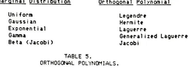
on.

A

possible solution

is

to

code

the

variables

using

orthogonal polynomi

als.

For

instance,

the

linear

terms

can

be

represented

by

Pl(x),

the

second order

terms

by

P2(x),

etc.

To

get

the

coefficients,

it

will

be

necessary

to decode

back,

into

the

original variable space.

The

choice of orthogonal polynomial

for

each variable should

be

deter

12

Maroinal

Distribution

Orthooonal

Polynomial

Uniform

Legendre

Gaussian

Hermite

Exponential

Laguerre

Gamma

Generalized Laguerre

Beta

(Jacobi)

Jacobi

TABLE

5.

ORTHOGONAL POLYNOMIALS.

However,

this

approach might prove

to

be

more

bother

than

it

is

worth.

The

investigator

must

first

select

the

proper set of

polynomials,

recode

the

data,

perform

the

analysis,

then

de-code

back

into

the

original

variable space.

Nonetheless,

it

should provide a

high

degree

of

linear

independence

between

the

powers of

the

same variable.

(Complete

orthog

onality

is

not necessary.)

-2.

The

number of "added*

variables

becomes

too

large.-

While

the

_vari

ables are partitioned

into

two

sets

(original

and

added),

and

hopefully

each partition

is

of more manageable size

than

with

the

old

approach,

nevertheless we are

left

with a

large

number of

total

variables,

as

indicated

in

Table

4.

The

major objection

to

this

problem

is

of course

the

enormous computational

load for

a

NLPCA

of a practical size.

-3.

A

singularity

in

either partition stops

the

process.-

In

Equations

(8)

and

(9)

we see

that

the

covariance matrices

for

both

partitions must

be

inverted

to

obtain

the

matrices

from

which

the NLPCA

coefficients are

determined.

When

machine computation

is

used,

a singular covariance

matrix

from

either

the

original or added partitions will cause

"MATRIX

SINGULAR

-CAWOT

INVERT"

or some similar epithet

to

be

printed out -and

the

computer run

halted.

It

is

necessary,

then,

to

eliminate

the

singularities

in

advance,

before

applying

Equations

(8)

and

(9).

Preliminary

Rotation

on each Partition-

To

solve

this,

together

with

the

problem

discussed

in

point

2

above,

the

author recommends

running

a preliminary

linear

principal component analysis on each partition.

This

not only allows

the

removal of

the

singularities

from

the

matrices

to be

inverted,

but

also allows

the

principal of parsimony

to

be

applied.

Naturally,

a complete canonical

decomposition

of

the

covariance matrix

for

the

original

data

would

be

performed.

If

any

linear

singularities

should

arise,

they

would naturally

be

of

interest.

The

remaining

principal components would

then

form

the

"original"

partition

for

the

canonical regression.

The

augmented variables would

be

examined

for

singularities similarly.

However,

because

it

was already pointed out

that

there

are

bound

to

be

near singularities

in

the

augmented partition

anyway,

these

singularities

[image:21.533.127.458.90.208.2]

13

course

be

when a perfect

singularity

occured,

which would

be

indicated

by

a

determinant

of zero.

In

order

to have

at

least

as

many

non-linear principal components as

there

were original

variates,

it

is

necessary

to

extract at

least

as

many

vectors

from

the

covariance matrix

for

the

added variables as

there

are

linearly

independent

columns of

the

covariance matrix of

the

original variables.

This

is

because

the

number of

functions

possible

from

a canonical regression

is

limited

by

the

size of

the

smallest partition.

If

there

were

p

original variates

in

the

problem,

then,

at

least

p

vectors should

be

extracted

from

the

covariance matrix of

the

added

var

iables.

Perhaps

a good rule of

thumb

for

greater

than

2

original variates would

simply

be

to double

this number,

so

2p

linear

principal components

be

extracted

from

the

covariance matrix of

the

added variables.

This

would

produce partitions sized no

larger

than

p

and

2p

.

The

largest

size of

these

partitions

is

presented

in

Table

6,

along

with

the

size of

the

matrix

to be

reckoned with under

the

old

method,

for

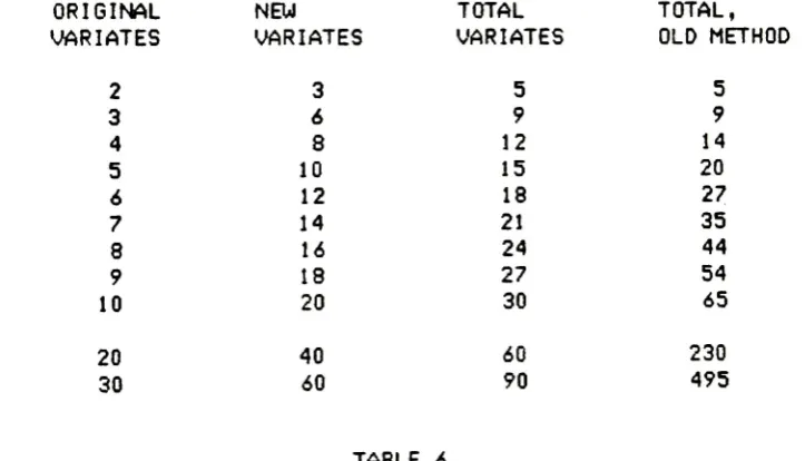
comparison purposes.

ORIGINAL

NEW

TOTAL

TOTAL,

VARIATES

VARIATES

VARIATES

OLD METHOD

2

3

5

5

3

6

9

9

4

8

12

14

5

10

15

20

6

12

18

27

7

14

21

35

8

16

24

44

9

18

27

54

10

20

30

65

20

40

60

230

30

60

90

495

TABLE

6.

COMPARISON

OF

DIMENSIONALITY

OF

MATRICES

FOR

OLD

AND NEW

METHODS.

It

is

interesting

to

note

that

the

total

size of

the

problem

increases

linearly

with respect

to

the

number of original

variates,

while

the

size

of

the

problem

for

the

old method

increases

quadrat

ical

1y.

This

becomes

especially

important

as

the

number of original variates reaches a

practical size

(say,

20

or

30).

Using

linear

principal component analysis

in

this

way as a precursor

to

the

non-linear principal component analysis would seem

to

make

the

use of [image:22.533.83.445.326.533.2]

14

In

computing

the

covariance matrix

for

the

transformed

variables,

it

should

be

remembered

that

the

upper

left-hand

corner

(the

covariance

matrix

for

the

transformed

original variables) will

be

a

diagonal

matrix,

because

of

the

orthogonality

of

the

linear

principal components.

Further,

these

diagonal

elements are

simply

the

eigenvectors correspon

ding

to

the

vectors extracted.

ESTIMATING

THE

MULTIPLICATIVE

CONSTttfT-Once

the

vectors

defining

the

canonical variates

have

been

determined,

it

is

necessary

to

determine

a multiplicative constant

for

each vector.

The

method used

to

estimate

the

relative contribution of each partition on

the

non-linear principal component

depends

on what

the

component

is

to

be

used

for.

If

we are

considering

the

vectors

first

extracted

from A

and

B,

we are

looking

for

relationships

among

the

variables,

and orthogonal regression

should

be

used.

However,

for

the

subsequent

functions (if

extracted),

the

first

linear

principal component should

be

used

instead

to

provide

maximum variance.

GENERAL

PROCEDURE

FOR NON-LINEAR

PRINCIPAL

COMPONENT

ANALYSIS-At

this point,

it

seems

that

a general procedure

for

non-linear principal

component analysis can

be

presented:

1.

Augment

the

original var

iables

wi

th

higher

order

terms

(square

and cross-product

terms)

2.

Compute

covariance matrices

for

both

original and added variables

3.

Perform

linear

principal component analysis on each partition.

-Complete analysis on original variate set

-At

least

p

vectors

(preferably

2p)

from

added set

4.

Compute

covariance matrix

for

new

transformed

variables

5.

Partition

into

original and added sets

6.

Obtain

canonical correlation coefficients

7.

Transform

back

into

original variate space

8.

Run

Orthogonal

Regression

on

functions

defined

by

canonical

variates

to

determine

multiplicative constants

15

CHAPTER FOUR

EXPERIMENTAL

METHOD

While

it

would

be

desirable

to

test

this

new approach with actual

data

from

a non-linear regression problem

containing

a

large

number of

predictors,

or some other practical

problem,

time

and space constraints

make

this

type

of experiment unreasonable.

Therefore,

we shall

limit

the

experiment

here

to

two

or

three

small problems.

The

first

problem

to

be

analyzed via

the

new method will

be

the

Gnanadesikan/Wi Ik

problem presented

in

Chapter

1

of

this

thesis,

in

Tables

1,

2,

and

3.

This

will provide a

direct

comparison

between

the

old and new approaches.

(In

order

to

prevent confusion

between

the

analysis of

the

Gnanadesi kan/Wi Ik

data

by

the

new method and

the

example

already published

by

Gnanadesikan

and

Wilk,.

the

analysis

by

the

new

method will

be

referred

to

as a solution of

the

'Gnanadesikan/Wi Ik

Problem",

rather

than

the

"Gnanadesikan/Wi Ik

Example",

as was used

for

their

solution.)

The

second problem

the

author would

like

to

analyze

j_s be

a

two

parameter

non-linear regression problem.

The

two

variates which would

form

the

basis

for

that

study would

be

the

partial

derivatives

of

the

model with

respect

to

the

two parameters,

evaluated at

the

least-squares

estimates

of

the

parameters.

Two

partial

derivatives

would

be

computed,

then,

for

each experimental unit

in

the

regression problem.

The

regression model

would

be

E(w)

= _v[l

-exp(-ut)],

which

has

particular significance

in

the

author's endeavors

in

ink

film

thickness

to

optical

density

conversions.

The

significance of

running

a non-linear principal component analysis on

the

derivatives

of a non-linear regression problem can probably

best

be

illustrated

by

pointing

out

the

analogies

between

linear

and non-linear

regression.

In

linear

regression,

the

covariance matrix of

the

parameter

estimates

is

obtained

by

multiplying

the

inverse

of

the X'X

matrix

by

the

residual mean-squares

for

residuals.

In

non-linear

regression,

the

covariance matrix

for

the

parameter estimates

is

approximated

by

multiplying

the

inverse

of

the

X'X

matrix

by

the

mean-sauares

for

residuals.

The

X'X

matrix

in

non-linear regression

is

computed

from

the

derivatives

of

the

model with respect

to

the

parameters

to be

estimated.

Just

as a

linear

principal component analysis would

be

run on

the

predic

tors

in

a

linear

regression,

a non-linear principal component analysis

would

be

run on

the

derivatives

in

a non-linear regression.

For

this

second

problem,

it

should

be

pointed out

that

no

data

need

be

collected;

this

problem concerns

itself

purely with

the

choice of

parameter values and ordinates.

The

primary goal of

this

phase of

the

study would

be

to

demonstrate

how

the

method of

NLPCA

by

canonical cor

16

Additionally,

it

would

be

desirable

to

obtain some

handle

on

the

signifi

cance of

the

second and subsequent

functions

to

be

extracted.

Because

of

the

nature of

NLPCA,

the

functions

should not

be

expected

to

reconstruct

the

data.

The

plethora of second-degree

terms

would make

solving for

the

original variables given

the

principal components a

formidable

task.

Also,

do

the

vectors

in

the

null space of

the

B

matrix

have

any

17

CHAPTER FIVE

EXPERIMENTAL RESULTS

GNANADESIKAN/WILK

PROBLEM-The

data

analyzed

by Gnanadesikan

and

Wilk,

presented earlier

here

in

Table

1,

was analyzed via

the

new method

by

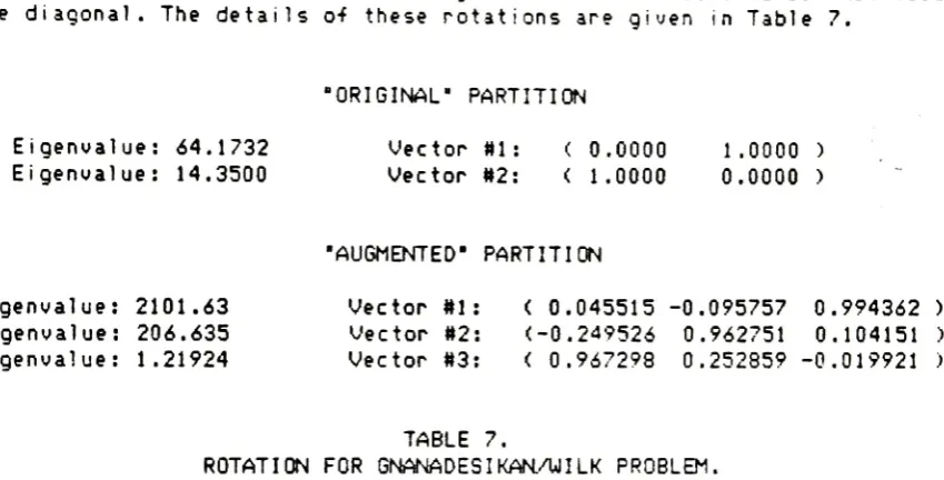
way of comparison.

The

first

step

in

the

analysis was

the

rotation of

the

partitions

to

two

sets of

variables

that

are

internally

orthogonal

-so

their

covariance matrices are

diagonal.

The

details

of

these

rotations are given

in

Table

7.

'ORIGINAL"

PARTITION

Eigenvalue:

64.1732

Eigenvalue:

14.3500

Vector

Vector

Ml:

tt2:

0000

0000

1.0000

)

0.0000

)

AUGMENTED*

PARTITION

Eigenvalue:

2101.63

Eigenvalue:

206.635

Eigenvalue:

1.21924

Vector

Ml:

(

0.045515

-0.095757

0.994362

)

Vector

2:

(-0.249526

0.962751

0.104151

)

Vector

3:

(

0.967298

0.252859

-0.019921

)

TABLE

7.

ROTATION FOR

GNANADESIKAN/WILK PROBLEM,

The A

and

B

matrices

(Equations

(8)

and

(9))

were

then

computed

using

the

happy

expediency of

the

orthogonality of

the

rotations,

which yielded

diagonal

covariance matrices and , which were easy

to

invert.

See

Table

8

for

the

matrices

A

and

B.

A

rttTRIX

[

0.965934

0.038164

-0.0085

0.9904S5

341

35J

B MATRIX

0.965633

-0.028952

1.527215

-0.002847

0.918823

-3.319163

0

.000886 -0 .019585

0

.071963

TABLE

8.

[image:26.533.42.467.188.404.2] [image:26.533.114.378.497.670.2]

18

These

two

matrices were

then

canonically

decomposed

to

yield

the

canoni

cal variate

pairs,

which were

then

transformed back

into

the

unrotated

variables

by

multiplying

the

vectors

by

the

transpose

of

the

rotation

matrices.

A

small orthogonal regression was run on

the

first

canonical

variate pair

to

obtain

the

multiplicative constants.

The

second non-linear principal component was extracted

from

the

trans

pose of

the

matrices

A

and

B.

Recall

that

the

linear

principal components

are orthogonal

to

each other.

The

situation analogous

to

this

in

the

non

linear

case would

be

the

orthogonality

of

the

gradient vectors

(see

Equation

(7)).

Unfortunately,

the

eigenvectors of matrices

A

and

B,

while

linearly

independent,

will not

be

orthogonal,

because

A

and

B

are not

real symmetric.

The

second non-linear principal component should

be

chosen so

that

the

second set of vectors

be

orthogonal

to

the

first

set.

Fortunately,

the

"left

hand"

eigenvectors of a matrix

(the

eigenvectors of

the

transpose)

have

a property called

"bi-orthogonal i

ty"

with

the

regular

("right

hand")

eigenvectors,

which means

that

the

i-th

left

hand

eigenvector of a matrix will

be

orthogonal

to

all

the

right-hand eigen

vectors except

the

i-th.

10]

This

would

tend

to

indicate

that

the

second non-linear principal component would come

from

the

transpose

of

the

matr

ices

A

and

B.

Further,

the

multiplicative constants should

be

estimated

by

a

linear

principal component analysis of

the

2

canonical variates obtained

from

the

second eigenvectors of

the

transpose

of

the

matrices

A

and

B.

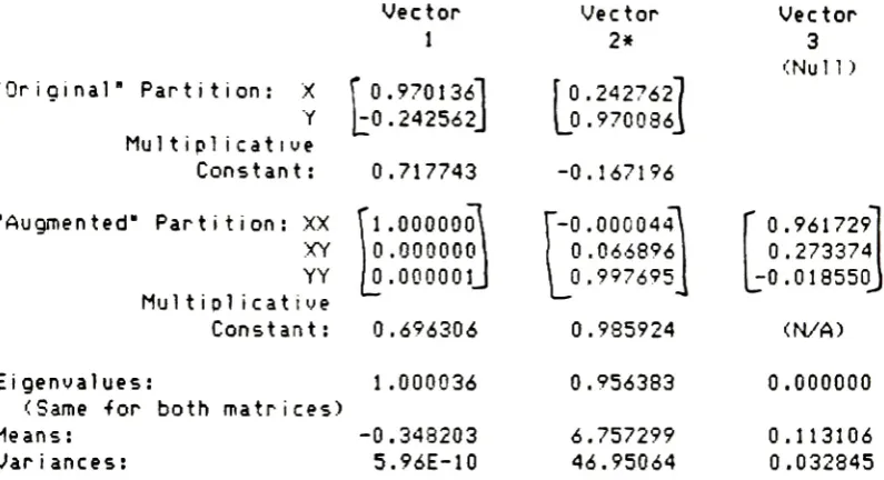
The

two

non-linear principal

components,

together

with

the

vector

in

the

null

space of

B,

are

in

Table

9.

It

should

be

noted

that

the

vectors presented

in

Table

9

have

already

been

transformed back

into

the

"untransf

ormed*

variable space of

X

and

Y,

and

XX,

XY,

and

YY,

rather

than

in

the

rotated variables obtained

by

the

linear

Drincipal component analysis on each partition.

It

was

felt

that

if

the

vectors originally

extracted,

in

the

"transformed"

variable

space,

were

to be

reported

also,

this

would unnecessarily clutter

the

table.

An

eigenvalue of

1.000036

is

reported

for

the

firs* non-linear princioal

component.

This

would

tend

to

indicate

rounding

error,

for

the

maximum

possible

is

one,

which corresponds

to

a unit squared canonical correla

tion

coefficient.

However,

a singularity

is

postulated

by

the

very

1

ow

variance of

the

first

non-linear principal component.

Note

that

the

function

obtained via canonical regression

is

very close

to

the

true

model

4X

-Y

+

4XX

+2=0.

The

extremely small value

for

the

variance of

this

function

tends

to

indicate

an almost exact

fit.

As

was pointed out

before,

the

second non-linear principal comoonent is of rather

limited

utility,

because

non-linear principal components

are,

by

their

nature,

not

in

general reconstructive of

the

original

data.

However,

the

second non-linear principal component

has

been

presented

19

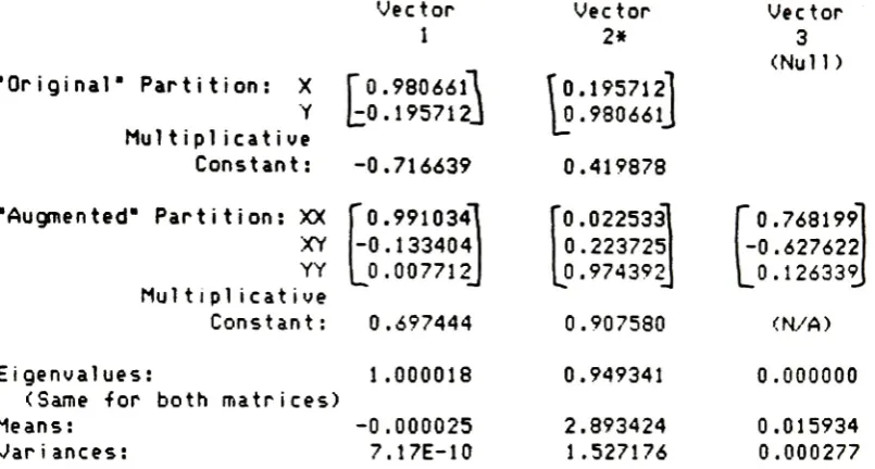
Finally,

the

third

vector of

the

B

matrix

is

presented.

Because

the

rank of

B

is

two,

the

third

eigenvalue

is

necessarily

zero,

so

the

third

eigenvector comes

from

the

null space of

B.

Note

that

a near singularity

exists

here

also,

as

indicated

by

the

relatively

small variance of

this

function,

compared

to

the

original variances.

Vector

1

Original"

Partition:

X

fo.

9701361

Y

[^0.242562]

Multiplicative

Constant

: Augmented"

Partition:

XX

XY

YY

Mul t i

pi

icat

i

ve

Constant

:

0.717743

l.ooooool

0.000000

0.000001J

0.696306

1.000036

Eigenvalues:

(Same

for

both

matrices)

Means:

-0.348203

Variances:

5.96E-10

Vector

2*

'0.242762]

L0.970086J

Vector

3

(Null)

-0.167196 -0.000044\

0.066896

0.997695J

'

0.961729

0.273374

j-0.018550.

0.985924

(N/A)

0.956383

0.000000

6.757299

46.95064

0.113106

0.032845

*2nd

vectors are

from

the

transposes

of

A

and

B

to

provide orthogonality.

FIRST

NON-LINEAR

PRINCIPAL

COMPONENT

Function:

0.696308

X

-0.174097

Y

?

0.696306

XX

+

0.348203

=

₀

Variance:

5.96

E-10

SECOND

NON-LINEAR

PRINCIPAL

COMPONENT

0.000043

XX

+

0.065954 XY

Function:

Z

= _-0.040589

X

-0.162194

Y

?

0.983651

YY

-

6.757299

Variance:

46.95064

TABLE

9.

NON-LINEAR

PRINCIPAL

COMPONENT

ANALYSIS

OF

GNANADESIKAN/WILK

PROBLEM.

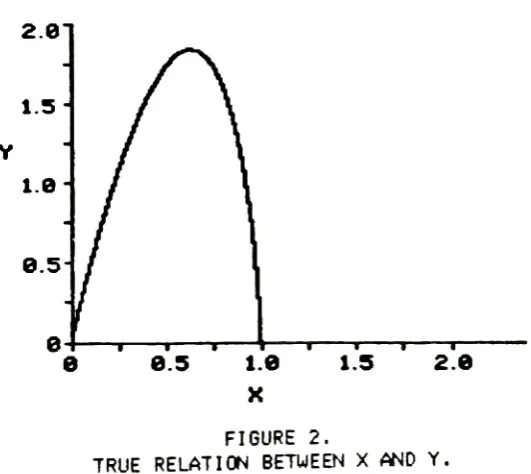
NON-LINEAR

REGRESSION

EXAMPLE-The

derivatives

in

non-linear regression problems constitute an examole [image:28.533.50.448.166.382.2]

20

most

from

the

technique

presented

here,

so a problem of

this

genre will

be

addressed

by

the

new

technique.

The

model

(10)

E(w)

= _v[l

-exp(-ut)]

is

particularly

important

in

ink-film

thickness

to

optical

density

con

versions as

the Tol

lenaar-Ernst model,

in

electricity

(RL

and

RC

time

curves),

physiology

(spirometer

curves),

and

in

many other physical

processes.

It

is

a

two-parameter

model,

with

the

first

parameter v

the

"saturation

value"

for

the

response,

w.

The

second

parameter,

u,

indicates

the

rate

at which

the

saturation value

is

reached as

the

independent

variable,

t,

is

increased.

XX

XY

YY

0.0

0.000000

0.000000

0.000000

0.000000

0.000000

0.5

0.095163

0.452419

0.009056

0.043053

0.204683

1.0

0.181269

0.818731

0.032859

0.148411

0.670320

1.5

0.259182

1

.111227

0.067175

0.288010

1.234826

2.0

0.329680

1.340640

0.108689

0.441982

1.797316

2.5

0.393469

1

.516327

0.154818

0.596628

2.299247

3.0

0.451188

1

.646435

0.203571

0.742852

2.710748

3.5

0.503415

1.738049

0.253426

0.874959

3.020813

4.0

0.550671

1

.797316

0.303239

0.989730

3.230344

4.5

0.593430

1.829563

0.352160

1.085718

3.347302

5.0

0.632121

1

.839397

0.399576

1.162721

3.383382

5.5

0.667129

1.830791

0.445061

1.221374

3.351796

6.0

0.698806

1.807165

0.488330

1.262858

3.265846

6.5

0.727463

1.771457

0.529210

1.288678

3.138059

7.0

0.753403

1.726179

0.567616

1.300508

2.979693

7.5

0.776870

1

.673476

0.603527

1.300073

2.800523

8.0

0.798103

1.615172

0.636969

1.289075

2.608781

8.5

0.817316

1.552810

0.668006

1.269137

2.411219

9.0

0.834701

1.487690

0.696726

1.241776

2.213222

9.5

0.850431

1.420902

0.723234

1.208380

2.018962

MEi^S

0.545691

1.448787

0.362162

0.887796

2.334354

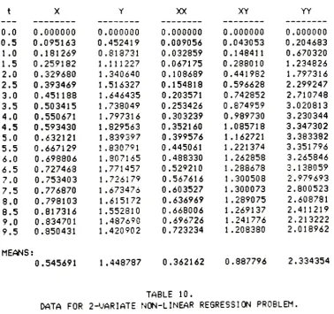
TABLE

10.

[image:29.533.80.459.278.633.2]

21

As

mentioned,

the

two

variates

to form

the

basis for

the NLPCA

will

be

the

two

partial

derivatives

of

(10)

with respect

to

the

two parameters,

v

and u.

These

are:

(11)

(12)

dv

The

values of

t

for

which

these

derivatives

will

be

evaluated were chosen

as

0

CO.

53

9.5,

with

the

values of v =

1

_{and u} =

0.2.

These

_{ordinates and}

parameter values were chosen so

that

the

maximum value of

t

would

represent

just

less

than

2

RL

or

RC

time

constants,

or,

alternatively,

an

ink

film

producing 85*/

relative optical

density.

These

data

appear

in

Table

10.

1.287678

1.944126

4.707390

XX

1.186987

1.446948

1.163019

XY

2.251627

3.720265

2.027608

4.125533

YY

3.968110

9.683242

2.980871

7.992721

21.17249

TABLE

11.

COVARIANCE

MATRIX

FOR

NON-LINEAR

REGRESSION PROBLEM.

The

covariance

matrix,

as

before,

multiplied

by

the

number of

degrees

of

freedom,

is

in

Table

11.

Table

12

contains

the

matrices

for

transforming

each partition

into

its

linear

principal

components,

and

the

canonical

regression matrices

A

and

B

are

in Table

13.

"ORIGINAL"

PARTITION

Eigenvalue:

5.586594

Eigenvalue:

0.408474

Vector

#1:

(

0.412058

0.911157

)

Vector

#2:

(

0.911157

-0.412053

)

Eigenvalue:

24.85652

Eigenvalue:

1.599312

Eigenvalue:

0.005129

AUGMENTED"

PARTITION

Vector

#1:

Vector

*2:

Vector

#3: