Strathprints Institutional Repository
Castaño, Adiel and Fernández-Navarro, Francisco and Riccardi, Annalisa
and Hervás-Martínez, Cesar (2016) Enforcement of the principal
component analysis - extreme learning machine algorithm by linear
discriminant analysis. Neural Computing and Applications, 27 (6). pp.
1749-1760. ISSN 0941-0643 , http://dx.doi.org/10.1007/s00521-015-1974-0
This version is available at http://strathprints.strath.ac.uk/58452/
Strathprints is designed to allow users to access the research output of the University of Strathclyde. Unless otherwise explicitly stated on the manuscript, Copyright © and Moral Rights for the papers on this site are retained by the individual authors and/or other copyright owners. Please check the manuscript for details of any other licences that may have been applied. You may not engage in further distribution of the material for any profitmaking activities or any commercial gain. You may freely distribute both the url (http://strathprints.strath.ac.uk/) and the content of this paper for research or private study, educational, or not-for-profit purposes without prior permission or charge.
Any correspondence concerning this service should be sent to Strathprints administrator:
Noname manuscript No. (will be inserted by the editor)
Enforcement of the Principal Component Analysis Extreme
Learning Machine Algorithm by Linear Discriminant Analysis
A. Casta˜no · F. Fern´andez-Navarro · Annalisa Riccardi · C.
Herv´as-Mart´ınez
Received: date / Accepted: date
Abstract In the majority of traditional Extreme Learn-ing Machine (ELM) approaches, the parameters of the basis functions are randomly generated and don’t need to be tuned while the weights connecting the hidden layer to the output layer are analytically estimated. The determination of the optimal number of basis functions to be included in the hidden layer is still an open prob-lem. Cross-validation and heuristic approaches (con-structive and de(con-structive) are some of the methodolo-gies used to perform this task. Recently, a deterministic algorithm based on the Principal Component Analysis (PCA) and ELM has been proposed to assess the num-ber of basis functions according to the numnum-ber of prin-cipal components necessary to explain the 90% of the variance in the data. In this work the PCA part of the PCA-ELM algorithm is joined to the Linear Discrimi-nant Analysis (LDA) as an hybrid means to perform the pruning of the hidden nodes. This is justified by the fact that the LDA approach is outperforming the PCA one on a set of problems. Hence the idea of combining the two approaches in a LDA-PCA-ELM algorithm that is
A. Casta˜no
Department of Computer Science, Universidad Polit´ecnica Salesiana Ecuador
E-mail: [email protected] F. Fern´andez-Navarro
Deparment of Mathematics and Engineering, Universidad Loyola Andalucia, Spain
E-mail: [email protected];[email protected], Annalisa Riccardi
Advanced Concepts Team, European Space Research and Technology Centre (ESTEC), European Space Agency (ESA), Noordwijk, Netherlands
E-mail: [email protected], C. Herv´as-Mart´ınez,
Department of Computer Science and Numerical Analysis, University of C´ordoba, Spain, E-mail: [email protected]
shown to be in average better than its PCA-ELM and LDA-ELM counterparts. Moreover the performance in classification and the number of basis functions selected by the algorithm, on a set of benchmark problems, have been compared and validated in the experimental sec-tion using non parametric tests against a set of existing ELM techniques.
Keywords Principal Component Analysis Linear Discriminant Analysis· Extreme Learning Machine·
Neural Networks
1 Introduction
The Extreme Learning Machine (ELM) framework has received much attention in the machine learning com-munity since Huang et. al [18, 17] proposed it in the In-ternational Joint Conference on Neural Networks. The ELM framework provides a way to estimate the pa-rameters of a Single-hidden Layer Feedforward Network (SLFN) analytically. The main idea of the framework is very intuitive and proceeds as follow: the parameters of the basis functions (also called hidden nodes) are randomly generated while the weights connecting the hidden layer to the output layer are analytically com-puted by inverting the hidden layer output matrix. The ELM does not require any iterations to determine the network parameters, reducing dramatically the compu-tational time. Thus, ELM is an highly compucompu-tationally efficient learning algorithm that provides good alization performance, even comparable to the gener-alization performance of the Support Vector Machine (SVM) [15]. The ELM framework has been successfully applied in facial expression recognition [28], engine air-ratio control [29] or electricity price classification [25] to name just a few of real-world applications.
Click here to view linked References
1 2 3 4 5 6 7 8 9 10 11 12 13 14 15 16 17 18 19 20 21 22 23 24 25 26 27 28 29 30 31 32 33 34 35 36 37 38 39 40 41 42 43 44 45 46 47 48 49 50 51 52 53 54 55 56 57 58 59 60
In the ELM framework, the determination of the optimal number of basis functions becomes an interest-ing and critical problem to exploit at most the ELM advantages. However, the original ELM [16] does not provide any effective solution to this problem. In most cases, the number of hidden nodes is part of a pre-processing analysis based on heuristics (trial and error or cross-validation procedures), a very tedious task in many real-world applications.
To avoid the aforementioned problems, some im-provements of the original ELM have been proposed to optimize the network architecture. The available method-ologies can be divided in two groups: destructive and constructive methods. For the former approach, Rong et al. [23] proposed the pruned ELM (P-ELM) for clas-sification problems. The algorithm is initialized with a large network and then removes the basis functions hav-ing low relevance to the output, in the meanhav-ing of small output layer weights. Miche et al. [22] proposed the Optimally-Pruned ELM (OP-ELM) algorithm which ran-domly initializes the hidden node weights, and ranks the resultant basis functions. The OP-ELM algorithm ap-plies the pruning strategy by the Multi-Response Sparse Regression (MRSR) algorithm and the Leave-One-Out (LOO) validation method. The main drawback of these destructive methods is that the algorithm starts with a large network that increases the computational com-plexity of the methodology. For the latter approach, the Incremental ELM (I-ELM) [15] and its variants [13, 14] are based on the idea of adding basis functions one-by-one to the hidden layer and incrementally update the output weights. The main problems of these algo-rithms are that those methods can not lead to an op-timal network architecture and the output weights of the SLFN are required to be recursively updated. On the other hand, Feng et al. [7] proposed the Error Mini-mized ELM (EM-ELM). The EM-ELM method can add random basis functions one-by-one or group-by-group. Unfortunately, the basis functions added are randomly generated and might deteriorate the performance with a large number of basis functions because no generaliza-tion performance is guaranteed. In a similar direcgeneraliza-tion, Lan et al. [19] proposed the Constructive Selection of hidden nodes in ELM (CS-ELM). In this approach, the basis functions are selected by the MRSR algorithm. However, the CS-ELM is suitable just for regression problems and the selection of the basis functions is car-ried out on normalized regressors (increasing the com-putational burden).
Furthermore, all constructive and destructive meth-ods for model selection of the ELM directly work on the basis function (hidden node) output matrix H ∈
RN ×RS, where N is the number of patterns in the
training set andS the number of basis functions. Gen-erally, the number of training patterns, N, is signif-icant higher than the number basis functios, S mak-ing theHmatrix potentially rank deficient and leading to unstable model structures. Finally, constructive and destructive methods limit the number of available ar-chitectures, thus introducing constraints in the search space of possible structures that may not be suitable to the problem. Although these methods have been proved useful in simulated data [27], their application to real problems has been rather unsuccessful [11].
Recently, Casta˜no proposed the Principal Compo-nent Analysis ELM (PCA-ELM) [4] where the basis functions are fitted taking into account the information retrieved from Principal Components Analysis. The PCA-ELM algorithm sets the number of basis functions by determining the amount of principal components (or-thogonal vectors) necessary to explain the 90% of the variance in the training set. The output node parame-ters are determined analytically using the Moore-Penrose generalized inverse as in the base ELM algorithm. This approach considerably decreases the computational cost compared to later ELM improvements, since no cross-validation is needed, and statistically outperform them. On the other hand, Linear Discriminant Analysis (LDA) has been used to reduce the dimensionality of the problem while maintaining the discriminability be-tween pre-defined classes [20]. The mathematical model of the LDA is a linear combination of the input patterns and the projections generated in the LDA. In the LDA algorithm, W ∈ RS ×RK is the matrix correspond-ing to theS largest eigenvectors of the matrixS−1
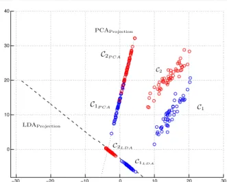
w Sb, where Sw is the within class scatter matrix and Sb is the between class scatter matrix. Sb is computed as the covariance matrix of the classes mean values while Sw is computed as the average of the classes covari-ance matrices. Thus it is assumed that the scatter of the data within class is the same for each class, unreal-istic assumption in practical problems, that still is able to lead to good performances in practical classification tests where the reduced LDA model is as effective or even more effective than the original one. Fig. 1 reports a 2 dimensional, 2 classes problem and the correspond-ing first PCA and LDA basis vectors. Clearly, as seen in this example, the two basis vectors define different projections and in particular, the projection of patterns onto the first LDA basis vector, is, in general, more ef-fective in discriminating between classes than the one provided by the first PCA vector.
This can be explained by the fact that the LDA al-gorithm makes direct use of the between classes covari-ance information while the PCA algorithm deals with the data as a whole, without including information on
1 2 3 4 5 6 7 8 9 10 11 12 13 14 15 16 17 18 19 20 21 22 23 24 25 26 27 28 29 30 31 32 33 34 35 36 37 38 39 40 41 42 43 44 45 46 47 48 49 50 51 52 53 54 55 56 57 58 59
−30 −20 −10 0 10 20 30 0 10 20 30 40
Fig. 1: Comparison of projections of PCA and LDA in a two-class classification problem: The classes are better separated by the projection onto the first LDA basis vector (w) than the projection onto the first PCA eigenvector.
the underlying class structure, into its analysis. Moti-vated by this fact, the LDA-PCA-ELM algorithm has been proposed, where the main difference with respect to the PCA-ELM method is that the hidden layer has been enlarged to include additional nodes for the LDA. It will be shown that the hybrid LDA-PCA approach in the ELM framework can improve the generalization performance of the model with respect to the two sin-gle analysis (PCA-ELM and LDA-ELM). This is due to the collaborative transformations applied by the two different analysis in the hidden nodes: while the LDA algorithm operates towards a better discrimination be-tween classes the PCA algorithm prefers a wide cover-age of the data space.
The paper is organized as follows: A background of LDA and PCA is given in Section 2. The methodology to optimize the SLFN parameters based on ELM and the joined LDA-PCA is presented in Section 3. Section 4 describes the experimental framework adopted to eval-uate the effectiveness of the method. Section 5 explains the results obtained. Finally, Section 6 summarizes the conclusions of the presented work.
2 Linear Discriminant Analysis and Principal Component Analysis
As previously stated, the main contribution of this work is the extension of the previously proposed PCA-ELM algorithm [4] by the Linear Discriminant Analysis (LDA) technique. The goal of this section is to establish the main differences of these two techniques. First the LDA
algorithm will be introduced and afterwards the PCA method will be described.
Note that the LDA technique uses the information of the targets in a classification problem. Because of that, the classification context is described. In a classifi-cation problem, given a single patternx= (x1, . . . , xK)∈
RK, its corresponding class label y ∈ {C1,C2, . . . ,CJ}
needs to be assessed, according to the learning per-formed on the available dataset. The training dataset D={X,Y}={(xn,yn)}Nn=1is considered, wherexn=
(x(1)n , . . . , x(nK)) ∈ RK is the vector of measurements,
and yn ∈RJ is the known class level of the n-th
pat-tern. In this work, the common technique to represent class levels using the “1-of-J” encoding vector is as-sumed, hence yn = (y
(1)
n , yn(2), . . . , yn(J)) with yn(j) = 1
in casexnis a pattern classified as classCj, 0 otherwise.
2.1 Linear Discriminant Analysis
LDA is a method used in pattern recognition and ma-chine learning to define a linear combination of fea-tures able to discriminate between two or more classes of patterns. LDA is also closely related to PCA which also seeks for linear combinations of features with the purpose of better separate the patterns. However the main difference between the two approaches is that LDA explicitly attempts to model the difference be-tween classes while PCA does not use targets informa-tion to perform the transformainforma-tions.
By applying LDA, the projections that maximize the distance between patterns of different classes and minimize the distance between patterns of the same class are found. In another words, the maximization of the between-class scatter matrixSb, together with the minimization of the within-class scatter matrix Sw in the projective subspace is performed. The within-class scatter matrix Sw ∈ RK ×RK and the between-class scatter matrixSb∈RK×RK are defined as:
Sw= J X j=1 X x∈Cj (x−xCj)(x−xCj) T, (1) Sb= J X j=1 (xCj −x)(xCj −x) T, (2) where xCj = (1/Nj) P
x∈Cjx is the mean of the j-th class with Nj the number of patterns belonging to it,
x = (1/N)PN
i=1xi is the mean of all patterns and J
is the number of classes. The goal is to maximize the variance between classes while minimizing the variance within class J(W) = argmax W WTS bW WTS wW . (3) 1 2 3 4 5 6 7 8 9 10 11 12 13 14 15 16 17 18 19 20 21 22 23 24 25 26 27 28 29 30 31 32 33 34 35 36 37 38 39 40 41 42 43 44 45 46 47 48 49 50 51 52 53 54 55 56 57 58 59 60
It has been proved already in [9] that, if Sw is a non singular matrix, then the maximum is attained by the matrixWthat has as column vectors the nonzero eigenvectors of the matrixS−1
w Sb, and they are at most
J −1. Hence the subspace for LDA is spanned by the set of vectors
W={w1,w2, . . . ,wJ−1} ∈RK×RJ−1. The main characteristics of LDA are:
– The new variables generally presents high separabil-ity between patterns of different classes and great union between same class ones.
– At most producesJ−1 feature projections.
2.2 Principal Component Analysis
PCA technique is an orthogonal transformation of the feature space that aims to find a set of linearly uncor-related components that better describes the variance between the data. In particular, the principal compo-nent is the vector that accounts for the greatest vari-ance while the following components are chosen with the same criteria but with the orthogonality constraint. Mathematically those vectors are the eigenvectors cor-responding to the largest eigenvalues of the dataset co-variance matrix. The data are further projected onto a subset of those directions for dimensionality reduction. If the matrix whose columns are the eigenvectors sorted according to the ascending order of the corre-sponding eigenvalues is denoted byU∈RK×RK, the PCA transformation of the data is
X=UTX,
where X= (x1, . . . ,xN)∈RK×RN denotes the
pat-terns matrix. By selecting only the first d rows of ˜X (with d ≤ K), the data have been projected from K down toddimensions.
The PCA technique has been traditionally imple-mented by the application of the Singular Value De-composition (SVD) of the patterns matrix X, defined as
X=ZΣVT
where V∈RN ×RN andZ∈RK×RK are orthonor-mal matrix,Σ∈RK×RN is a pseudo-diagonal matrix
whose diagonal entries are ordered in a descending order and they correspond to the eigenvalues of theXmatrix and the values outside the diagonal are zero. The eigen-vectors of the covariance matrix C= (1/N−1)XTXare
computed from theVmatrix since
XTX=VΣZTZΣVT =VΣ2VT and then C= 1 N−1 VΣ2VT. BeingC symmetric it stands that
C=VΛVT
where Λ is the diagonal matrix with eigenvalues ofC as entries values on the diagonal and the column of V as the corresponding eigenvectors. The eigenvalues and eigenvectors of the covariance matrix of the pattern matrix can then be easily computed by the elements of the SVD decomposition.
It is important also to stress the attention on the ne-cessity of performing the mean subtraction (also called “mean centering”) to ensure that during the PCA anal-ysis, the first principal component is not too close to the mean of the data, but describes the direction of maxi-mum variance.
The main characteristics of PCA can be summarized as:
– The features in the projected space are uncorre-lated.
– The covariance matrix represents only second order statistics among the vector values.
– Maximize variance of patterns in the projected space.
2.3 Why LDA can outperform PCA for classification tasks?
First of all, it is worth mentioning that in a classifica-tion problem of dimension K and J classes, the PCA methods estimateKprojections while the LDA method findsJ−1 projections. As previously noted, LDA uses targets information to improve the performance of the algorithms that applies LDA with respect to the same algorithms that instead makes use of PCA. To justify the proposed combination of LDA and PCA for clas-sification, the example in Fig. 1 is discussed. As can be seen, the patterns are distributed in a particular and not uncommon way. The PCA tries to maximize data variance while LDA finds the best projection that separates the classes. A joined combination of the two approaches can help in preserving distinction between classes and a good spread of the patterns within each class.
Due to the intuitive characteristics of LDA for clas-sification and the results obtained in previous works [4], where PCA transformations were included in the ELM framework, the integration of LDA into the PCA-ELM model is here proposed and discussed.
1 2 3 4 5 6 7 8 9 10 11 12 13 14 15 16 17 18 19 20 21 22 23 24 25 26 27 28 29 30 31 32 33 34 35 36 37 38 39 40 41 42 43 44 45 46 47 48 49 50 51 52 53 54 55 56 57 58 59
3 The proposed Method: Linear Discriminant Analysis-Principal Component Analysis Extreme Learning Machine (LDA-PCA-ELM) The goal of this section is to describe the proposed method, named Linear Discriminant Analysis-Principal Component Analysis Extreme Learning Machine (LDA-PCA-ELM). As shown in the experimental section, the algorithm is a suitable option to estimate the param-eters of SLFN. A SLFN is a type of neural network composed by three layers: a input, a hidden and an output layer. Let’s denote withas= (as1, as2, . . . , asK)T
the weight vector connecting the input units to thes-th hidden unit, s = 1, . . . , S, and βj = (β1j, βj2, . . . , βSj)T
is the weight vector connecting the hidden nodes to the j-th output node ∀j = 1,2, . . . , J. During the training process the optimal parameters:as, andβj, are
deter-mined so that they minimize the Squared Error (SE) function defined by:
SE= N X n=1 J X j=1 (fj(xn)−yn(j))2, (4)
where fj(xn) is the estimated output of thej-th class
for then-th input pattern, which is defined as: fj(xn) = S X s=1 βj sφs(xn;as) (5)
where φs(xn;as) is the sigmoidal activation function
in this work. The minimization of the squared error function in the ELM is achieved solving the following linear system:
Hβ=Y, (6)
whereHis known as the hidden layer output matrix of the SLFN and defined as:
H= (h1,h2, . . . ,hS) = = φ1(x1;a1). . . φS(x1;aS) . . . . φ1(xn;a1). . . φS(xn;aS) RN×RS , (7) Y = (y1,y2, . . . ,yn)TRN×RJ, (8) and β= (β1,β2, . . . ,βJ)RS×RJ. (9)
In the case of the standard ELM framework pro-posed by Huang et. al. [17] the parameters connecting the input layer to the hidden layer (as,∀s = 1, . . . , S)
are randomly determined, while the weights for the out-put layer are analytically comout-puted using the Moore-Penrose pseudoinverse matrix.
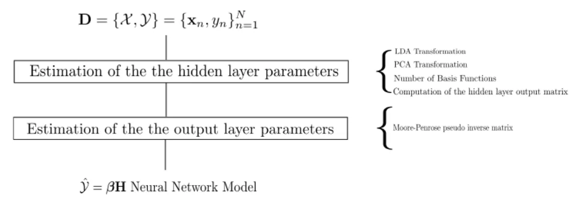
The main contribution of the proposed algorithm (LDA-PCA-ELM) is the initialization of the weights connecting the input layer to the hidden layer. In the LDA-PCA-ELM algorithm, these weights are initialized according to the combined LDA and PCA methods fit-ting the biases to zero. The LDA-PCA-ELM algorithm can be viewed as a two-stage algorithm as shown in Fig. 2.
3.1 Estimation of the hidden layer parameters
The first step of the LDA-PCA-ELM algorithm is the execution of the LDA and PCA algorithm over the data in the training set. Then, the parametersas, s=
1, . . . , S are initialized according to the basis projec-tion vectors generated by both the LDA and PCA ap-proaches. Taking into consideration that the maximum number of projections generated by the LDA areJ−1 and the maximum number of projections generated by the PCA are K, the maximum number of basis func-tions to be included in the SLFN isJ −1 +K. Hence S∈[1, J−1 +K].
The next step is the pruning step: in this work it is considered that the basis functions to be included in the SLFN must explain the 90% of the variance of the data in both approaches. This method prunes the model using the same mechanism used by PCA-ELM. Therefore, only those S1 basis functions that explain 90% or more of the variance of the data in the training set out of theJ−1 possible basis functions are included in the model for the LDA case and S2 basis functions that explain 90% or more of the variance of the data in the training set out of theKpossible basis functions are included in the model for the PCA case. Hence
S=S1+S2.
This deterministic technique to set the number of hidden nodes rises the complexity of the model with respect to random-based initialization of the ELM al-gorithms.
After that, the LDA-PCA-ELM proceeds by choos-ing an activation functionφ(x) to generate the hidden layer output matrixH. Among the existing hidden node types, the one composed by a linear activation function and a transfer function are considered in this work. Be-cause of this, any hidden node that is compounded by a linear combination as the activation function may be taken into consideration as a suitable choice to be used
1 2 3 4 5 6 7 8 9 10 11 12 13 14 15 16 17 18 19 20 21 22 23 24 25 26 27 28 29 30 31 32 33 34 35 36 37 38 39 40 41 42 43 44 45 46 47 48 49 50 51 52 53 54 55 56 57 58 59 60
Fig. 2: LDA-PCA-ELM Framework ( ˆY is the estimated outputs of the model)
in the hidden layer of the SLFN. Some of the most com-mon hidden nodes with a linear activation function are mentioned hereafter:
– Sigmoidal Function (Sig): in particular, the special case of the logistic function, defined as:
sig(n) = 1
1 + exp(−n). (10)
– Hard-limit transfer function (Hardlim): it returns one for nonzero negative values, zero otherwise: hardlim(n) =
1 ifn≥0
0 otherwise (11)
– Sine (Sin): it returns zero for values close to 2Kπ. In order to validate our algorithm and for the sake of simplicity the experiments are only done using sig-moidal nodes in the hidden layer.
3.2 Estimation of the output layer parameters
Finally, the estimation of the output layer weights is done as proposed by Huang [17], solving the linear sys-tem Hβ =Y using the Moore-Penrose generalized in-verse. In this way, the values of the β parameters are estimated as:
β=H†Y (12)
where H† is the Moore-Penrose generalized inverse of the hidden layer output matrix. It has also been shown that this solution is the least-square solutions of the general linear system Hβ =Y, therefore it minimizes the training error. Moreover it is unique, and has the smallest norm of weights, hence having also good gen-eralization performance [17, 5].
Table 1 summarizes the algorithmic steps of the base ELM algorithm and the LDA-PCA-ELM method and highlights their main differences.
3.3 Discussion about the Advantages of the LDA-PCA-ELM
The LDA-PCA-ELM proposed algorithm is an exten-sion of the previously proposed PCA-ELM algorithm and it inherits some of the most important advantages of the PCA-ELM and the good properties of LDA with respect to the state-of-the-art ELM approaches:
1. The algorithm is deterministic instead of stochastic. This implies that the algorithm does not present a high standard deviation of its performance and model complexity as OP-ELM and other algorithms do.
2. Previously proposed approaches determine the op-timal number of basis functions by growing or prun-ing techniques. These techniques are generally hard time consuming. The proposed approach determines the amount of hidden nodes taking into considera-tion the cumulative variance expressed in the LDA and PCA algorithms.
The main drawback of the proposed method with respect to the PCA-ELM is that PCA-ELM can ap-plied to regression and classification problems, while LDA-PCA-ELM can be applied only to classification problems because LDA uses information of the targets, trying to maximize the distance between classes and minimize the distance within class.
4 Experimental Framework
In this section, the setting of the experimental study performed is presented. Section 4.1 lists the datasets tested; Section 4.2 provides a description of the met-rics used to evaluate the performance of the algorithms; Section 4.3 presents the list of algorithms implemented for comparison together with their parameters; finally, Section 4.4 describes the statistical tests performed to validate the obtained results.
1 2 3 4 5 6 7 8 9 10 11 12 13 14 15 16 17 18 19 20 21 22 23 24 25 26 27 28 29 30 31 32 33 34 35 36 37 38 39 40 41 42 43 44 45 46 47 48 49 50 51 52 53 54 55 56 57 58 59
ELM LDA-PCA-ELM 1. Assign arbitrary input weightsas,s= 1, . . . , S.
2. Calculate the hidden layer output matrixH.
3. Calculate the output weightsβ:β=H†Y.
whereH,βandY are as defined before.
1. Execute LDA and PCA over the training set. 2. Select the optimal number of transformations. 3. Calculate the hidden layer output matrixH.
4. Calculate the output weightsβ:β=H†Y.
Table 1: Main differences of the ELM algorithm with respect the LDA-PCA-ELM algorithm
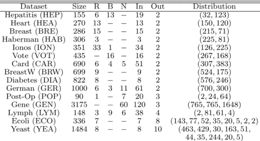
4.1 Datasets considered
The proposed algorithm was tested on fifteen datasets taken from the UCI repository [1]. The datasets selected range from binary problems to multi-class problems, they present a variety of size, number of features and number of classes. Table 2 summarizes the characteris-tics of the datasets used. In particular the size of the datasets vary from 90 to 3175 patterns, the number of features ranges from 3 to 120. They have been parti-tioned using a hold-out cross-validation procedure with 3/4·n instances for the training dataset and n/4 in-stances for the generalization set. To account for the aleatory nature of the ELM stochastic approaches 1, those algorithms were run 30 times for each problem. The ELM deterministic approaches (PCA-ELM, LDA-ELM and LDA-PCA-LDA-ELM algorithms) were run just one time per dataset. In addition, instances with miss-ing values have been discarded before the execution of the methods over the datasets and the whole set of val-ues have been normalized in the interval [0,1] to uni-form the sensitivity of attributes with different range domains.
4.2 Evaluation metrics
Two metrics were used to assess the performance of each method:
– Accuracy rate (Acc): It is the number of success-ful hits (correct classifications) relative to the total number of classifications. It is the most widely used metric.
– Number of Hidden Nodes (N HN): In this work we use the N HN to measure the complexity of the neural networks models. Taking into account that all the methods considered work with fully con-1 By ELM stochastic approaches we are naming to those
ELM-based methodologies where the hidden layer parameters are randomly initialized. In this study the only deterministic methodologies considered are those that initialize the hidden layer parameters according to the LDA or PCA projections (or a combination of both)
Dataset Size R B N In Out Distribution Hepatitis (HEP) 155 6 13 − 19 2 (32,123) Heart (HEA) 270 13 − − 13 2 (150,120) Breast (BRE) 286 15 − − 15 2 (215,71) Haberman (HAB) 306 3 − − 3 2 (225,81) Ionos (ION) 351 33 1 − 34 2 (126,225) Vote (VOT) 435 − 16 − 16 2 (267,168) Card (CAR) 690 6 4 5 51 2 (307,383) BreastW (BRW) 699 9 − − 9 2 (524,175) Diabetes (DIA) 822 8 − − 8 2 (576,246) German (GER) 1000 6 3 11 61 2 (700,300) Post-Op (POP) 90 1 − 7 20 3 (2,24,64) Gene (GEN) 3175 − − 60 120 3 (765,765,1648) Lymph (LYM) 148 3 9 6 38 4 (2,81,61,4) Ecoli (ECO) 336 7 − − 7 8 (143,77,52,35,20,5,2,2) Yeast (YEA) 1484 8 − − 8 10 (463,429,30,163,51, 44,35,244,20,5) All nominal variables are transformed to binary variables.
Table 2: Characteristics of the datasets used for the ex-periments: number of instances (Size), number of Real (R), Binary (B) and Nominal (N) input variables, total number of inputs (In.), number of classes (Out.), and per-class distribution of the instances (Distribution)
nected neural networks, theN HNis a robust metric to estimate the complexity of the model.
Additionally, the time required to estimate the pa-rameters of each method has been also considered. The time (T) is the simplest way to estimate the compu-tational efficiency of the methods. The average time elapsed (in seconds) is considered, this includes cross-validation, training and test time.
4.3 ELM algorithms selected
The proposed method (LDA-PCA-ELM) is compared to the following ELM approaches:
– The Cross-Validated original Extreme Learning Ma-chine (ELMCV) [17]. In this method, the number of hidden nodes in the base ELM algorithm has been selected by a nested five fold cross-validation proce-dure over the training set, i.e., once the lowest cross-validation error alternative was obtained, it was ap-plied to the complete training set and test results were extracted. The criteria for selecting the best
1 2 3 4 5 6 7 8 9 10 11 12 13 14 15 16 17 18 19 20 21 22 23 24 25 26 27 28 29 30 31 32 33 34 35 36 37 38 39 40 41 42 43 44 45 46 47 48 49 50 51 52 53 54 55 56 57 58 59 60
configuration was theAccperformance. The values considered in the cross-validation procedure were
{10,20, . . . ,100}. The sigmoidal non linear trans-formation was the basis function considered for the hidden layer.
– The Optimally Pruned Extreme Learning Machine (OP-ELM) [21]. The OP-ELM extends the original ELM algorithm wrapping it around with a method-ology that prunes the hidden neurons, leading to a more robust overall algorithm. Again, the sigmoidal non-linear transformation was the one considered in this study. The number of nodes (S) in the hidden layer in the OP-ELM algorithm is set at the begin-ning to 100, since this algorithm prunes the useless neurons from the hidden layer.
– The Cross-Validated Evolutionary Extreme Learn-ing Machine (E−ELMCV) [30, 3, 24] improves the original ELM by using a Differential Evolution (DE) algorithm [26] and determines the optimal number of hidden nodes by a cross-validation procedure. The E−ELMCV uses the evolutionary technique to optimize the input weights and the Moore-Penrose generalized inverse to analytically determine the out-put weights.
In the same way as in the ELM algorithm, the most critical parameter in the E−ELMCV algorithm is the number of the hidden nodes,S. The number of hidden nodes was selected with a cross-validation procedure based on a set of nodes multiple of 10 ({10,20, . . . ,100}). To widely explore the search space a populaion of 100 individuals is used in the evolu-tionary procedure, for a maximum number of gener-ations equal to 50. The E−ELMCV algorithm has been implemented using the sigmoidal unit as the basis function in the hidden layer.
– The Incremental Extreme Learning Machine (I-ELM) [15]. This algorithm proposes a procedure that in-creases the network architecture adding random nodes till the residual error is bigger than a threshold. This threshold must be set in advance and its value is very sensible to the number of patterns and classes. The algorithm was initially proposed for regression but can be extended for classification.
– The Pruned Extreme Learning Machine (P-ELM) [23] uses statistical methods to measure the rele-vance of hidden nodes. Hidden nodes are ranked us-ing statistical techniques such as chi-square and in-formation gain. Irrelevant nodes are then pruned by considering their relevance to the class labels. The optimal number of hidden nodes is estimated con-sidering the performance of the classifier on a (strat-ified) validation set constructed with the 25% of the training set patterns as suggested by the authors.
– The Error Minimized Extreme Learning Machine (EM-ELM) [7]. The main difference of this algo-rithm with respect to the I-ELM method resides in the computation of the output layer weights which are estimated with the goal of improving the com-putational burden of the previously mentioned al-gorithm. The algorithm is strongly sensitive to an error threshold parameter which depends on number of patterns, classes and hidden nodes. A hyper pa-rameter was introduced in the model to implement a fair experimental comparison with respect to the remaining methods. The new hyper-parameter was defined as the relative error with respect to the num-ber of patterns and classes. The hyper-parameter space was explored by considering a cross-validation procedure based on a set of hidden nodes multiple of 10 ({10,20, . . . ,100}).
– The Principal Component Analysis Extreme Learn-ing Machine (PCA-ELM) [4]. This algorithm does not have any hyper-parameter to be estimated by cross-validation. As explained before, the number of hidden nodes, S, is estimated according to the accumulated variance expressed into the eigenvec-tors.
– The Linear Discriminant Analysis Extreme Learn-ing Machine (LDA-ELM). This algorithm has been also included to prove that the combination of LDA and PCA is able to outperform its single counter-parts.
4.4 Statistical Tests
Hypothesis testing techniques is a useful tool to statisti-cally interpret the results obtained in the experimental study and discriminate between methods according to their performance [6]. Non parametric tests have been chosen over parametric ones, for this specific case, be-cause the initial conditions that guarantee the reliabil-ity of the second ones may not be satisfied, entailing the statistical analysis to lose plausibility.
In particular, the Friedman pre-hoc test, is used. Its application can outline significant differences between the methods tested. Moreover The Holm posthoc pro-cedures will detect which algorithms are significant to be used for comparisons.
5 Experiments
5.1 Analysis of generalization performance
For the sake of simplicity, only the graphical and the summary of the statistical results achieved are included,
1 2 3 4 5 6 7 8 9 10 11 12 13 14 15 16 17 18 19 20 21 22 23 24 25 26 27 28 29 30 31 32 33 34 35 36 37 38 39 40 41 42 43 44 45 46 47 48 49 50 51 52 53 54 55 56 57 58 59
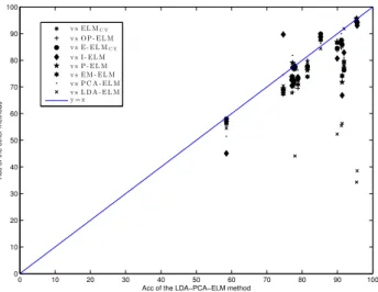
whereas the complete results can be found at the url www.esa.int/act/LDA-PCA-ELM.zip. 0 10 20 30 40 50 60 70 80 90 100 0 10 20 30 40 50 60 70 80 90 100
Acc of the LDA−PCA−ELM method
Acc of the other methods
v s E L MC V v s O P - E L M v s E - E L MC V v s I - E L M v s P - E L M v s E M - E L M v s P C A - E L M v s L D A - E L M y = x
Fig. 3: Graphical results of the generalization perfor-mance
In the scatterplot of Fig. 3, each point compares LDA-PCA-ELM to another methodology on a single dataset. LDA-PCA-ELM was considered as the base method because it reported the best mean results. The x-axis position of the point is the mean performance of LDA-PCA-ELM of one dataset, and the y-axis position is the performance of the compared algorithm (using
Acc). Therefore, points below they=xline correspond to datasets for which LDA-PCA-ELM performs better than the other algorithm when the metric should be maximized (Acc) and points above they =xline rep-resent to datasets for which LDA-PCA-ELM achieves a better performance than the compared method when the metric should be minimized (N HN metric).As can be seen in Fig. 3, the LDA-PCA-ELM is a competitive methodology if it is compared to the most promising approach (the PCA-ELM method). From the analysis of the results (Table 3), it can be concluded that the LDA-PCA-ELM model produces the best mean rank-ing in Acc (RAcc = 2.10), reporting also the highest
mean accuracy (Acc= 82.91%).
The non-parametric Friedman test [10], using as test variable theAcc value computed in the generalization set of the best models, has been performed to deter-mine the statistical significance of the rank differences reported for each method in the different datasets. The test shows that the effect of the method used for classi-fication is statistically significant at a significance level of 10%.
Based on this rejection, the Holm post-hoc test was used to compare all classifiers with a control method
Method Acc RAcc z-statistic p-value α ′ Holm LDA-ELM 63.35 7.00 4.90 0.000 0.012 EM-ELM 77.85 6.06 3.96 7.0E-5 0.014 OP-ELM 77.43 5.73 3.63 2.8E-4 0.016 ELMCV 78.51 5.13 3.10 0.001 0.020 I-ELM 78.50 5.06 3.03 0.024 0.025 E−ELMCV 78.99 5.20 2.96 0.030 0.033 P-ELM 78.49 4.86 2.76 0.005 0.050 PCA-ELM 80.63 3.70 1.73 0.080 0.100 LDA-PCA-ELM 82.91 2.10 -
-Best results in bold face; second best in italics
Table 3: Statistical results using Acc as the variable test: Mean Acc in the generalization set (Acc), mean ranking (RAcc), z-statistic for the Holm post-hoc test,
p-value and corrected alpha (α′Holm) for the same test
[12]. For the experiments carried out, the control method selected is the one reporting the best mean ranking in Acc, the LDA-PCA-ELM method. The results of the Holm test forα= 0.10 can be seen in Table 3. By us-ing a level of significance α = 0.10, LDA-PCA-ELM is significantly better than the rest of the algorithms consideredexcept PCA-ELM.
5.2 Analysis of model complexity
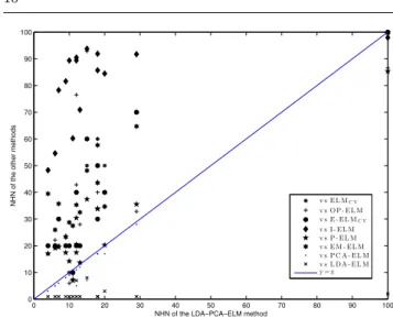
In this section, a graphical plot of the number of hid-den nodes (N HN) is shown. Fig. 4 is thescatter plot representation of theN HN included in each model for the methodologies considered. As can be seen in Fig. 4, the LDA-PCA-ELM is a competitive method when compared to the state-of-the-art ELM methods.As can be seen the most algorithms are located over the diago-nal line indicating that are more complex models. From a purely descriptive point of view, we can see how the LDA-PCA-ELM methods obtains the third best mean ranking and overall N HN (Table 4). The additional performance gains for including the LDA transforma-tions in the hidden layer justifies the inclusion of these transformation in the final model (despite on increase in the model complexity).
It is necessary though to determine if there are dif-ferences in the mean ranking ofN HN. Hence another non-parametric Friedman test has been performed, show-ing that the effect of the method used for classification is statistically significant at a significance level of 10%, as the confidence interval isC0= (0, F0.05= 2.02)and
the F-distribution statistical values are F∗ = 45.12 ∈/ C0 forN HN. Accordingly, the null-hypothesis stating
that all algorithms perform equally in mean ranking is rejected.
On the basis of this rejection, the Holm post-hoc test is used to compare all the methods to a given con-trol method. The differences in rankings between the
1 2 3 4 5 6 7 8 9 10 11 12 13 14 15 16 17 18 19 20 21 22 23 24 25 26 27 28 29 30 31 32 33 34 35 36 37 38 39 40 41 42 43 44 45 46 47 48 49 50 51 52 53 54 55 56 57 58 59 60
0 10 20 30 40 50 60 70 80 90 100 0 10 20 30 40 50 60 70 80 90 100
NHN of the LDA−PCA−ELM method
NHN of the other methods v s E L MC V
v s O P - E L M v s E - E L MC V v s I - E L M v s P - E L M v s E M - E L M v s P C A - E L M v s L D A - E L M y = x
Fig. 4: Graphical results of the complexity of the models considered (according to the number of hidden nodes, NHN)
Method N HN RNHN z-statistic p-value α ′ Holm I−ELM 80.57 1.33 7.53 0.000 0.012 EM−ELM 41.16 3.13 5.73 0.000 0.014 ELMCV 37.33 3.63 5.23 0.000 0.016 E−ELMCV 36.67 3.76 5.1 0.000 0.020 OP-ELM 38.99 4.30 4.56 2.0E-5 0.025 P-ELM 26.82 5.93 2.93 0.003 0.033 LDA-PCA-ELM 18.93 6.30 2.56 0.102 0.050 PCA-ELM 16.80 7.73 1.13 0.257 0.100 LDA-ELM 2.06 8.86 - - -Best results in bold face; second best in italics
Table 4: Statistical results usingN HN as the variable test: MeanN HN selected in the training step (N HN), mean ranking (RNHN),z-statistic for the Holm post-hoc test, p-value and corrected alpha (α′Holm) for the same test
different algorithms and the results of the Holm test for α = 0.100 is reported in Table 4, using the corre-spondingp-values. By using this test, it can be seen that the LDA-ELM method significantly outperforms the re-maining methods (excepts the PCA-ELM method).
5.3 Time Complexity Analysis
The time complexity of the proposed algorithm is an-alyzed in this subsection. The LDA-PCA-ELM algo-rithm is composed by three main time consuming tasks:
– Computation of the LDA vectors. – Computation of the PCA eigenvectors.
– Determination of the Moore-Penrose pseudo-inverse matrix.
The LDA hasO(nkt+t3) time complexity and re-quiresO(nk+nt+kt) memory, wherenis the number
Computation Time
ELMCV 0.010 P-ELM 0.066
OP-ELM 0.540 EM-ELM 0.239 E−ELMCV 62.606 PCA-ELM 0.016
I-ELM 0.155 LDA-ELM 0.038 Control method LDA-PCA-ELM†: 0.061
Table 5: Mean training time over all the datasets (T) of the different methods considered
of training patterns, k is the number of features and t =min(n, k) [2]. When both n and k are large, it is difficult to apply LDA. On the other hand, the PCA has O(nk2) time complexity. Obviously, the proposed ap-proach (LDA-PCA-ELM) is more time consuming that the baseline algorithm considered (PCA-ELM), taking into account thatn >> kin most of the real-world ap-plications and that it requires the computation also of the LDA vectors. Finally, the inversion of a sizeN×N matrix has a complexity ofO(N2log(N)).
Table 5 reports the average running time (consid-ering also the cross-validation and the test time) of the algorithms considered. All the experiments were run using a common Matlab framework proposed in [8, 24]. The proposed algorithm was developed and in-cluded in the above-mentioned framework. In general, the most efficient algorithm is the base ELM. Despite this, the proposed method achieved a competitive com-putational time, specially if it is compared to EM-ELM2, OP-ELM and E−ELMCV algorithms.
5.4 Sensitivity Analysis
The proposed algorithm relies mainly on only one hy-peparameter: the Percentage of Variance Explained (PVE) by the LDA and PCA projections, used to determine the Number of Hidden Nodes (N HN). In the experi-mental study, the number of projections considered are those that explain the 90% of PVE. A study has been performed to analyze the sensitivity of the model, in terms of Accuracy (Acc), with respect to this hyper-parameter (percentage of variance explained) to justify the setup decision. The datasets selected for the study are those with the maximum number of possible projec-tions (those with the maximum value ofJ−1 +K) and they are: theCard (52 possible projections),Ionos (35 possible projections), Gene (122 possible projections) andGerman(62 possible projections) datasets. Several runs of the LDA-PCA-ELM algorithm have been per-formed for values of the the hyperparameter ranging in
2
The computational burden of EM-ELM was seen severely affected by the estimation of the threshold parameter
1 2 3 4 5 6 7 8 9 10 11 12 13 14 15 16 17 18 19 20 21 22 23 24 25 26 27 28 29 30 31 32 33 34 35 36 37 38 39 40 41 42 43 44 45 46 47 48 49 50 51 52 53 54 55 56 57 58 59
the set: PVE∈ {10,20,40,60,90,100} (13) 10 20 30 40 50 60 70 80 90 100 70 72 74 76 78 80 82 84 86 88 90
Percentage of Variance Explained
A cc Card German Ionos Gene
Fig. 5: Hypeparameter study onAccfor the LDA-PCA-ELM algorithm and the PVE parameter.
Results are reported in Fig. 5. As expected the gen-eralization performance of LDA-PCA-ELM tends to mono-tonically increase with the PVE. In general, as observed from Fig. 5, the best performance values are obtained with a PVE of 90% (which is also true for the other datasets). There is only few exceptions to this rule and all of them would lead to slightly increase the gen-eralization performance by increasing significantly the N HN. For example, for the Genedataset, the model gets a 84.23% of generalization performance for PVE equal to 90% and a 86.12% of generalization perfor-mance for PVE equal to 100%. However in the first case N HN = 100 while in the second case N HN = 122. Therefore, in order to reduce the complexity of the al-gorithm, the PVE parameter can be directly set to 90%.
6 Conclusions
In this work, the Linear Discriminant Analysis-Principal Component Analysis-Extreme Learning Machine (LDA-PCA-ELM) algorithm is proposed. As shown in the experiments, the proposal is a fast and robust ELM-based algorithm. The LDA-PCA-ELM algorithm esti-mates the parameters of the hidden layer according to the eigenvector and the projections generated by the PCA and LDA algorithms respectively. As in the base ELM method, the weights connecting the hidden and
the output layer are estimated analytically according to the Moore-Penrose pseudo-inverse matrix. The pro-posed algorithm is validated using fifteen well-known classification datasets. The results obtained are statis-tically compared using the Holm and Friedman tests. This statistical analysis indicates that the proposed ap-proach is a competitive method in time and in number of hidden nodes, improving the previous methods es-pecially in overall accuracy. The main limitation of the methodology proposed with respect to traditional ELM approaches is that ELM algorithms can be applied to several problems including classification and regression problems or even to unsupervised learning problems while LDA-PCA-ELM algorithm can be applied only to classification problems because LDA needs informa-tion about the classificainforma-tion labels.
References
1. Asuncion, A., Newman, D.: UCI machine learning repos-itory (2007). URL http://www.ics.uci.edu/~mlearn/ MLRepository.html
2. Cai, D., He, X., Han, J.: Training linear discriminant analysis in linear time. Data Engineering, International Conference on0, 209–217 (2008)
3. Cao, J., Lin, Z., Huang, G..: Composite function wavelet neural networks with differential evolution and extreme learning machine. Neural Processing Letters33(3), 251–
265 (2011)
4. Casta˜no, A., Fern´andez-Navarro, F., Herv´as-Mart´ınez, C.: Pca-elm: A robust and pruned extreme learning ma-chine approach based on principal component analysis. Neural Processing Letters37(3), 377–392 (2013)
5. Chen, L., Zhou, L., Pung, H.K.: Universal approxima-tion and qos violaapproxima-tion applicaapproxima-tion of extreme learning machine. Neural Processing Letters28(2), 81–95 (2008)
6. Demˇsar, J.: Statistical comparisons of classifiers over mul-tiple data sets. Journal of Machine Learning Research7,
1–30 (2006)
7. Feng, G., Huang, G.B., Lin, Q., Gay, R.: Error minimized extreme learning machine with growth of hidden nodes and incremental learning. IEEE Transactions on Neural Networks20(8), 1352–1357 (2009)
8. Fern´andez-Navarro, F., Herv´as-Mart´ınez, C., S´ anchez-Monedero, J., Gutierrez, P.A.: MELM-GRBF: A mod-ified version of the extreme learning machine for gener-alized radial basis function neural networks. Neurocom-puting74(16), 2502–2510 (2011)
9. Fisher, R.: The statistical utilization of multiple measure-ments. Annals of Eugenics8, 376–386 (1938)
10. Friedman, M.: A comparison of alternative tests of sig-nificance for the problem ofmrankings. Annals of Math-ematical Statistics11(1), 86–92 (1940)
11. Hassibi, B., Stork, D.G., et al.: Second order derivatives for network pruning: Optimal brain surgeon. Advances in neural information processing systems pp. 164–164 (1993)
12. Hochberg, Y., Tamhane, A.: Multiple Comparison Pro-cedures. John Wiley & Sons (1987)
13. Huang, G.B., Chen, L.: Convex incremental extreme learning machine. Neurocomputing 70(16-18), 3056 –
3062 (2007) 1 2 3 4 5 6 7 8 9 10 11 12 13 14 15 16 17 18 19 20 21 22 23 24 25 26 27 28 29 30 31 32 33 34 35 36 37 38 39 40 41 42 43 44 45 46 47 48 49 50 51 52 53 54 55 56 57 58 59 60
14. Huang, G.B., Chen, L.: Enhanced random search based incremental extreme learning machine. Neurocomputing
71(16-18), 3460–3468 (2008)
15. Huang, G.B., Chen, L., Siew, C.K.: Universal approxima-tion using incremental constructive feedforward networks with random hidden nodes. IEEE Transactions on Neural Networks17(4) (2006)
16. Huang, G.B., Zhou, H., Ding, X., Zhang, R.: Extreme learning machine for regression and multiclass classifica-tion. IEEE Transactions on Systems, Man, and Cyber-netics, Part B42(2), 513–529 (2012)
17. Huang, G.B., Zhu, Q., Siew, C.: Extreme learning ma-chine: Theory and applications. Neurocomputing70
(1-3), 489–501 (2006)
18. Huang, G.B., Zhu, Q.Y., Siew, C.K.: Extreme learning machine: A new learning scheme of feedforward neural networks. In: IEEE International Conference on Neural Networks - Conference Proceedings, vol. 2, pp. 985–990 (2004)
19. Lan, Y., Soh, Y.C., Huang, G.B.: Constructive hidden nodes selection of extreme learning machine for regres-sion. Neurocomputing73(16–18), 3191 – 3199 (2010)
20. Mart´ınez, A.M., Kak, A.C.: Pca versus lda. IEEE Trans-action on Pattern Analysis and Machine Intelligence
23(2), 228–233 (2001)
21. Miche, Y., Sorjamaa, A., Bas, P., Simula, O., Jutten, C., Lendasse, A.: OP-ELM: Optimally Pruned Extreme Learning Machine. IEEE Transactions on Neural Net-works21(1), 158–162 (2010)
22. Miche, Y., Sorjamaa, A., Lendasse, A.: Op-elm: Theory, experiments and a toolbox. In: Artificial Neural Networks - ICANN 2008,Lecture Notes in Computer Science, vol. 5163, pp. 145–154. Springer Berlin / Heidelberg (2008) 23. Rong, H.J., Ong, Y.S., Tan, A.H., Zhu, Z.: A fast
pruned-extreme learning machine for classification problem. Neu-rocomputing72(1-3), 359 – 366 (2008)
24. S´anchez-Monedero, J., Guti´errez, P.A., Fern´ andez-Navarro, F., Herv´as-Mart´ınez, C.: Weighting efficient ac-curacy and minimum sensitivity for evolving multi-class classifiers. Neural Processing Letters 34(2), 101–116
(2011)
25. Shrivastava, N., Panigrahi, B., Lim, M.H.: Electricity price classification using extreme learning machines. Neu-ral Computing and Applications pp. 1–10 (2014) 26. Storn, R., Price, K.: Differential evolution. a fast and
efficient heuristic for global optimization over continu-ous spaces. Journal of Global Optimization11, 341–359
(1997)
27. Thodberg, H.H.: Improving generalization of neural net-works through pruning. International Journal of Neural Systems1(04), 317–326 (1991)
28. Ucar, A., Demir, Y., G¨uzeli¸s, C.: A new facial expres-sion recognition based on curvelet transform and on-line sequential extreme learning machine initialized with spherical clustering. Neural Computing and Applications (2014)
29. Wong, P., Wong, H., Vong, C., Xie, Z., Huang, S.: Model predictive engine air-ratio control using online sequential extreme learning machine. Neural Computing and Ap-plications (2014)
30. Zhu, Q.Y., Qin, A., Suganthan, P., Huang, G.B.: Evolu-tionary extreme learning machine. Pattern Recognition
38(10), 1759 – 1763 (2005) 1 2 3 4 5 6 7 8 9 10 11 12 13 14 15 16 17 18 19 20 21 22 23 24 25 26 27 28 29 30 31 32 33 34 35 36 37 38 39 40 41 42 43 44 45 46 47 48 49 50 51 52 53 54 55 56 57 58 59