PRINCIPAL COMPONENT ANALYSIS FOR
SECOND-ORDER STATIONARY VECTOR TIME SERIES
By Jinyuan Chang1,∗ , Bin Guo1,† and Qiwei Yao2,‡
Southwestern University of Finance and Economics1, and London School of Economics and Political Science2
We extend the principal component analysis (PCA) to second-order stationary vector time series in the sense that we seek for a contemporaneous linear transformation for a p-variate time series such that the transformed series is segmented into several lower-dimensional subseries, and those subseries are uncorrelated with each other both contemporaneously and serially. Therefore those lower-dimensional series can be analyzed separately as far as the linear dynamic structure is concerned. Technically it boils down to an eige-nanalysis for a positive definite matrix. Whenpis large, an additional step is required to perform a permutation in terms of either maxi-mum cross-correlations or FDR based on multiple tests. The asymp-totic theory is established for both fixed p and diverging p when the sample sizentends to infinity. Numerical experiments with both simulated and real data sets indicate that the proposed method is an effective initial step in analyzing multiple time series data, which leads to substantial dimension reduction in modelling and forecasting high-dimensional linear dynamical structures. Unlike PCA for inde-pendent data, there is no guarantee that the required linear transfor-mation exists. When it does not, the proposed method provides an approximate segmentation which leads to the advantages in, for ex-ample, forecasting for future values. The method can also be adapted to segment multiple volatility processes.
1. Introduction. Modelling multiple time series, also called vector time series, is always a challenge, even when the vector dimensionpis moderately large. While most the inference methods and the associated theory for uni-variate autoregressive and moving average (ARMA) processes have found
∗Supported in part by the Fundamental Research Funds for the Central Universities (Grant No. JBK160159, JBK150501), NSFC (Grant No. 11501462), the Center of Statis-tical Research at SWUFE, and the Joint Lab of Data Science and Business Intelligence at SWUFE.
†Supported in part by the Fundamental Research Funds for the Central Universities (Grant No. JBK120509, JBK140507) and the Center of Statistical Research at SWUFE.
‡Supported in part by an EPSRC research grant. Primary 62M10; secondary 62H25
Keywords and phrases: α-mixing, autocorrelation, cross-correlation, dimension reduc-tion, eigenanalysis, high-dimensional time series, weak stationarity.
their multivariate counterparts (L¨utkepohl, 2006), vector autoregressive and moving average (VARMA) models are seldom used directly in practice when p≥3. This is partially due to the lack of identifiability for VARMA models in general. More fundamentally, those models are overparametrized; leading to flat likelihood functions which cause innate difficulties in statistical infer-ence. Therefore finding an effective way to reduce the number of parameters is particularly felicitous in modelling and forecasting multiple time series. The urge for doing so is more pertinent in this modern information age, as it has become commonplace to access and to analyze high dimensional time series data with dimension p in the order of hundreds or more. Big time series data arise from, among others, panel study for economic and natural phenomena, social network, healthcare and public health, financial market, supermarket transactions, information retrieval and recommender systems. Available methods to reduce the number of parameters in modelling vec-tor time series can be divided into two categories: regularization and di-mension reduction. The former imposes some conditions on the structure of a VARMA model. The latter represents a high-dimensional process in terms of several lower-dimensional processes. Various regularization meth-ods have been developed in literature. For example, Jakeman, Steele and Young (1980) adopted a two stage regression strategy based on instrumen-tal variables to avoid using moving average explicitly. Different canonical structures are imposed on VARMA models [Chapter 3 of Reinsel (1993), Chapter 4 of Tsay (2014), and references within]. Structural restrictions are imposed in order to specify and to estimate some reduced forms of vector autoregressive (VAR) models [Chapter 9 of L¨utkepohl (2006), and refer-ences within]. Davis, Zang and Zheng (2012) proposed a VAR model with sparse coefficient matrices based on partial spectral coherence. Under dif-ferent sparsity assumptions, VAR models have been estimated by LASSO regularization (Shojaie and Michailidis, 2010; Song and Bickel, 2011), or by the Dantzig selector (Han and Liu, 2013). Guo, Wang and Yao (2016) con-sidered high-dimensional autoregression with banded coefficient matrices. The dimension reduction methods include the canonical correlation anal-ysis of Box and Tiao (1977), the independent component analanal-ysis (ICA) of Back and Weigend (1997), the principal component analysis (PCA) of Stock and Watson (2002), the scalar component analysis of Tiao and Tsay (1989) and Huang and Tsay (2014), the dynamic orthogonal components analysis of Matteson and Tsay (2011). Another popular approach is to rep-resent multiple time series in terms of a few latent factors defined in various ways. There is a large body of literature in this area published in the outlets in statistics, econometrics and signal processing. An incomplete list of the
publications includes Anderson (1963), Pe˜na and Box (1987), Tong, Xu and Kailath (1994), Belouchrani et al. (1997), Bai and Ng (2002), Theis, Meyer-Baese and Lang (2004), Stock and Watson (2005), Forni et al. (2005), Pan and Yao (2008), Lam, Yao and Bathia (2011), Lam and Yao (2012) and Chang, Guo and Yao (2015).
A new dimension reduction method is proposed in this paper. We seek for a contemporaneous linear transformation such that the transformed series is segmented into several lower-dimensional subseries, and those subseries are uncorrelated with each other both contemporaneously and serially. Therefore they can be modelled or forecasted separately, as far as linear dependence is concerned. This reduces the number of parameters involved in depicting lin-ear dynamic structure substantially. While the basic idea is not new, which has been explored with various methods including some aforementioned ref-erences, the method proposed in this paper (i.e. the new PCA for time series) is new, simple and effective. Technically the proposed method boils down to an eigenanalysis for a positive definite matrix which is a quadratic function of the cross correlation matrix function for the observed process. Hence it is easy to implement and the required computation can be carried out with, for example, an ordinary personal computer or laptop for the data with dimensionp in the order of thousands.
The method can be viewed as an extension of the standard PCA for multiple time series, therefore, is abbreviated as TS-PCA. However the seg-mented subseries are not guaranteed to exist as those subseries must not correlate with each other across all times. This is a marked difference from the standard PCA. The real data examples in Section 4 indicate that it is often reasonable to assume that the segmentation exists. Furthermore, when the assumption is invalid, the proposed method provides some approximate segmentations which ignore some weak though significant correlations, and those weak correlations are of little practical use for modelling and forecast-ing. Thus the proposed method can be used as an initial step in analyz-ing multiple time series, which often transforms a multi-dimensional prob-lem into several lower-dimensional probprob-lems. Chang, Yao and Zhou (2017) demonstrates that such an initial transformation increases the power in test-ing for high-dimensional white noise. Furthermore the results obtained for the transformed subseries can be easily transformed back to the original multiple time series. Illustration with real data examples indicates clearly the advantages in post-sample forecasting from using the proposed TS-PCA. TheR-package PCA4TS, available from CRAN project, implements the
pro-posed methodology.
is the same in principle as the ICA using autocovariances presented in Sec-tion 18.1 of Hyv¨arinen, Karhunen and Oja (2001). However, the nonlinear optimization algorithms presented there are to search for a linear transfor-mation such that all the off-diagonal elements of the autocovariance matrices for the transformed vector time series are minimized. See also Tong, Xu and Kailath (1994), and Belouchrani et al. (1997). To apply those algorithms to our setting, we need to know exactly the block diagonal structure of auto-covariances of the transformed vector process (i.e. the number of blocks and the sizes of all the blocks), which is unknown in practice. Furthermore, our method is simple and fast, and therefore is applicable to high-dimensional cases. Cardoso (1998) extends the basic idea of ICA to the so called multi-variate ICA, which requires the transformed random vector to be segmented into several independent groups with possibly more than one component in each group. But Cardoso (1998) does not provide a pertinent algorithm for multivariate ICA. Furthermore it does not consider the dependence across different time lags. TS-PCA is also different from the dynamic PCA pro-posed in Chapter 9 of Brillinger (1981) which decomposes each component time series as the sum of moving averages of several uncorrelated white noise processes. In our TS-PCA, no lagged variables enter the decomposition.
The rest of the paper is organized as follows. The methodology is spelled out in Section 2. Section 3 presents the associated asymptotic properties of the proposed method. Numerical illustration with real data are reported in Section 4. Section 5 extends the method to segmenting a multiple volatil-ity process into several lower-dimensional volatilvolatil-ity processes. Some final remarks are given in Section 6. All technical proofs and numerical illus-tration with simulated data are relegated to the supplementary material [Chang, Guo and Yao (2017)]. We always use the following notation. For any m × k matrix H = (hi,j), let kHk2 = λ1max/2 (HHT) and kHkF =
(Pmi=1Pkj=1hi,j2 )1/2, where λmax(HHT) denotes the largest eigenvalue of
HHT.
2. Methodology.
2.1. Setting and method. Let yt be observable p×1 weakly stationary
time series. We assume that yt admits a latent segmentation structure:
(2.1) yt=Axt,
wherextis an unobservablep×1 weakly stationary time series consisting of
q(>1) both contemporaneously and serially uncorrelated subseries, andA is an unknown constant matrix. Hence all the autocovariances of xt are of
the same block-diagonal structure with q blocks. Denote the segmentation ofxt by
(2.2) xt= (x(1)t ,T, . . . ,x
(q),T
t )T
with Cov(x(ti),x(sj)) =0 for allt, sandi6=j. Thereforex(1)t , . . . ,x(tq) can be
modelled or forecasted separately as far as their linear dynamic structure is concerned.
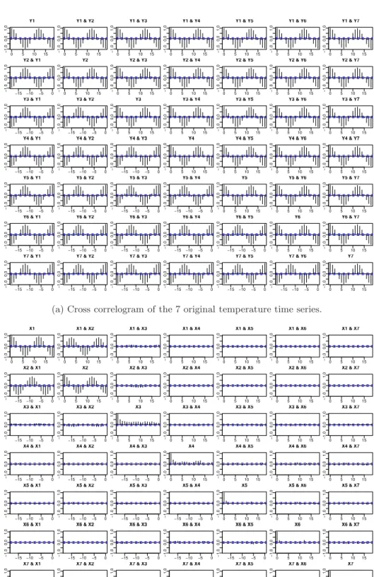
Example 1. Before we spell out how to find the segmentation
trans-formation A in general, we consider the monthly temperatures of 7 cities (Nanjing, Dongtai, Huoshan, Hefei, Shanghai, Anqing and Hangzhou) in Eastern China from January 1954 to December 1998. Fig 1(a) plots the cross correlations of these 7 temperature time series. Both the autocorrelation of each component series and the cross correlation between any two compo-nent series are dominated by the annual temperature fluctuation; showing the strong periodicity with the period 12. Now we apply the linear transfor-mationxt=Byt with B= 0.244 −0.066 0.019 −0.050 −0.313 −0.154 0.200 −0.703 0.324 −0.617 0.189 0.633 0.499 −0.323 0.375 1.544 −1.615 0.170 −2.266 0.126 1.596 3.025 −1.381 −0.787 −1.691 −0.212 1.188 −0.165 −0.197 −1.820 −1.416 3.269 0.301 −1.438 1.299 −0.584 −0.354 0.847 −1.262 −0.218 −0.151 1.831 1.869 −0.742 0.034 0.501 0.492 −2.533 0.339 .
See Section 4 below for howBis calculated. Fig 1(b) shows that the first two transformed component series are significantly correlated both concurrently and serially, and there are also small but significant correlations in the (3, 2)-th panel; indicating 2)-the linear dependence between 2)-the 2nd and 2)-the 3rd transformed component series. Apart from these, there is little significant cross correlation among all the other pairs of component series. This visual observation suggests to segment the 7 transformed series into 5 uncorrelated groups:{1, 2, 3}, {4},{5}, {6} and{7}.
This example indicates that the segmentation transformation transfers the problem of analyzing a 7-dimensional time series into the five lower-dimensional problems: four univariate time series and one 3-lower-dimensional time series. Those five time series can and should be analyzed separately as there are no cross correlations among them at all time lags. The linear dynamic
structure of the original series is deduced by those of the five transformed series, as Cov(yt+k,yt) =ACov(xt+k,xt)AT.
Now we spell out how to find the segmentation transformation under (2.1) and (2.2). Without the loss of generality we may assume
(2.3) Var(yt) =Ip and Var(xt) =Ip,
where Ip denotes the p× p identity matrix. This first equation in (2.3)
amounts to replaceyt by Vb−1/2yt as a preliminary step in practice, where
b
V is a consistent estimator for Var(yt). As both A and xt are
unobserv-able, the second equation in (2.3) implies that we view (A{Var(xt)}1/2, {Var(xt)}−1/2xt) as (A,xt) in (2.1). More importantly, the latter perspective
will not alter the block-diagonal structure of the autocovariance matrices of xt. Now it follows from (2.1) and (2.3) that Ip = Var(yt) =AVar(xt)AT=
AAT.Thus,Ain (2.1) is an orthogonal matrix under (2.3).
Let pj be the length of x(tj). Write A = (A1, . . . ,Aq), where Aj has pj
columns. Sincext=ATyt, it follows from (2.2) that
(2.4) x(tj)=AT
jyt, j = 1, . . . , q.
LetHj be any pj×pj orthogonal matrix, and H= diag(H1, . . . ,Hq). Then
(A,xt) in (2.1) can be replaced by (AH,HTxt) while (2.2) still holds. Hence
A and xt are not uniquely identified in (2.1), even with the additional
as-sumption (2.3). In fact under (2.3), only M(A1), . . . ,M(Aq) are uniquely
defined by (2.1), where M(Aj) denotes the linear space spanned by the
columns of Aj. Consequently, ΓTjyt can be taken as x(tj) for any p ×pj
matrixΓj as long as ΓTjΓj =Ipj and M(Γj) =M(Aj).
To discover the latent segmentation, we need to estimateA= (A1, . . . ,Aq),
or more precisely, to estimate linear spacesM(A1), . . . ,M(Aq). To this end,
we introduce some notation first. For any integerk, letΣy(k) = Cov(yt+k,yt)
andΣx(k) = Cov(xt+k,xt).For a prescribed positive integer k0, define
Wy = k0 X k=0 Σy(k)Σy(k)T =Ip+ k0 X k=1 Σy(k)Σy(k)T, (2.5) Wx= k0 X k=0 Σx(k)Σx(k)T=Ip+ k0 X k=1 Σx(k)Σx(k)T.
Then bothΣx(k) and Wx are block-diagonal, and
Note that bothWy andWx are positive definite matrices. Let
(2.7) WxΓx =ΓxD,
i.e.Γxis ap×porthogonal matrix with the columns being the orthonormal
eigenvectors of Wx, and D is a diagonal matrix with the corresponding
eigenvalues as the elements on the main diagonal. Then (2.6) implies that WyAΓx = AΓxD. Hence the columns of Γy ≡ AΓx are the orthonormal
eigenvectors ofWy. Consequently,
(2.8) ΓT
yyt=ΓTxATyt=ΓTxxt,
the last equality follows from (2.1). Put
(2.9) Wx = diag(Wx,1, . . . ,Wx,q).
ThenWx,j is apj×pj positive definite matrix, and the eigenvalues ofWx,j
are also the eigenvalues ofWx. Suppose that Wx,i and Wx,j do not share
the same eigenvalues for any i 6= j. Then if we line up the eigenvalues of Wx (i.e. the eigenvalues ofWx,1, . . . ,Wx,q combining together) in the main
diagonal ofDaccording to the order of the blocks inWx,Γxmust be a
block-diagonal orthogonal matrix of the same shape asWx; see Proposition 1(i).
However the order of the eigenvalues is latent, and anyΓx defined by (2.7)
is nevertheless a column-permutation (i.e. a matrix consisting of the same column vectors but arranged in a different order) of such a block-diagonal orthogonal matrix; see Proposition 1(ii). Hence each component ofΓT
xxtis a
linear transformation of the elements in one of theq subseries only, i.e. thep components of ΓT
yyt=ΓTxxt can be partitioned into theq groups such that
there exist neither contemporaneous nor serial correlations across different groups. ThusΓT
yyt can be regarded as a permutation of xt, andΓy can be
viewed as a column-permutation ofA; see the discussion below (2.4). This leads to the following two-step estimation forAand xt:
Step 1. LetSbbe an estimator forWy. Calculate ap×porthogonal matrix b
Γy with the columns being the orthonormal eigenvectors ofbS.
Step 2. The columns ofAb = (Ab1, . . . ,Abq) are a permutation of the columns
ofΓby such thatbxt=AbTyt is segmented intoq uncorrelated subseries b
x(tj)=AbT
jyt,j= 1, . . . , q.
Step 1 is the key, as it provides an estimator forAexcept that the columns of the estimator are not grouped together according to the latent segmentation. The estimatorSb should be consistent, and will be constructed under various scenarios in Section 3 below. The permutation in Step 2 above can be carried out in principle by visual observation: plot cross correlogram of bzt ≡ Γb
T
(using, for example,R-functionacf); see Fig 1(b). We then put those
com-ponents ofbzttogether when there exist significant cross-correlations (at any
lags) between those component series. ThenAb is obtained by re-arranging the order of the columns ofΓby accordingly.
Remark1. (i) Appropriate precaution should be exercised in the visual
observation stated above. First the visual observation become impractical whenpis large. Furthermore most correlogram plots produced by statistical packages (includingR) use the confidence bounds at ±1.96/√n for sample cross-correlations of two time series. Unfortunately those bounds are only valid if at least one of the two series is white noise. In general, the confidence bounds depend on the autocorrelations of the two series. See Theorem 7.3.1 of Brockwell and Davis (1996). In Section 2.2, we will describe how the permutation can be performed without the benefit of visual observation for the cross correlogram of bzt. Ledoit and Wolf (2004) and Paparoditis and
Politis (2012) provide more modern approaches to view correlations. (ii)Wy defined in (2.5) combines the information over different time lags
together. In practice we need to specify the integer k0. Note that all terms
on the right-hand side of (2.5) is non-negative definite. Hence there is no information cancellation over different lags. This makes the method insen-sitive to the choice of k0. In practice a small k0 is often sufficient, as long
as the first k0 lags carry sufficient information on the latent block
diago-nal structure even when the auto/cross-correlations beyond lag k0 are still
significant. The examples in Section 4 lend further support to this assertion.
Proposition 1. (i) The orthogonal matrix Γx in (2.7) can be taken as
a block-diagonal orthogonal matrix with the same block structure as Wx.
(ii)An orthogonal matrix Γx satisfies(2.7)if and only if its columns are a
permutation of the columns of a block-diagonal orthogonal matrix described in (i), provided that any two different blocks Wx,i and Wx,j do not share
the same eigenvalues.
Proposition 1(ii) requires that theq blocks ofWx do not share the same
eigenvalue(s). However it does not rule out the possibility that each block Wx,j may have multiple eigenvalues. When different blocks share the same
eigenvalue(s), Proposition 1 still holds with Wx replaced by Wx⋆ which is
also a block diagonal matrix with fewer thanqblocks obtained by combining together thoseWx,j’s sharing at least one common eigenvalue into one larger
block. This means that the proposed method will not be able to separate, for example, x(1)t and x(2)t if Wx,1 and Wx,2 share at least one common
2.2. Permutation.
2.2.1. Permutation rule. The columns of Ab is a permutation of the columns of Γby. The permutation is determined by grouping the
compo-nents ofbzt=Γb T
yyt intoq groups, whereqand the cardinal numbers of those
groups are unknown. Writezbt= (bz1,t, . . . ,zbp,t)T. Letρi,j(h) denote the cross
correlation between the two component serieszbi,t and zbj,t at lag h. We say
b
zi,t and bzj,t connectedif the multiple null hypothesis
(2.10) H0:ρi,j(h) = 0 for any h= 0,±1,±2, . . . ,±m
is rejected, wherem≥1 is a prescribed integer. Thus there exists significant evidence indicating non-zero correlations between two connected component series. Hence those components should be put in the same group. We may takem= 20, ormsufficiently large but smaller thann/4, in the spirit of the rule of thumb proposed by Box and Jenkins (1970, p.30), as we exclude long memory processes in this paper. Note that the autocorrelations of stationary (causal) VARMA processes decay exponentially fast. The permutation in Step 2 in Section 2.1 can be performed as follows.
i. Start with thepgroups with each group containing one component of
bztonly.
ii. Combine two groups together if one connected pair are split over the two groups.
iii. Repeat Step ii above until all connected pairs are within one group.
We introduce below two methods for identifying the connected pair compo-nents ofbzt=Γb
T
yyt.
2.2.2. Maximum cross correlation method. One natural way to test hy-pothesisH0 in (2.10) is to use the maximum cross correlation over the lags
between−mand m:
(2.11) Lbn(i, j) = max
|h|≤m|ρbi,j(h)|,
where ρbi,j(h) is the sample cross correlation between bzi,t and bzj,t at lag
h. We would reject H0 for the pair (bzi,t,bzj,t) if Lbn(i, j) is greater than an
appropriate threshold value.
Instead of conducting multiple tests for each of thep0≡p(p−1)/2 pairs
components ofbzt, we propose a ratio-based statistic to single out those pairs
for which H0 will be rejected. To this end, we re-arrange the p0 obtained
b
Ln(i, j)’s in the descending order: Lb1≥ · · · ≥Lbp0. Define
(2.12) rb= arg max
1≤j<c0p0
b
wherec0 ∈(0,1) is a prescribed constant. In all the numerical examples in
Section 4 and the supplementary material [Chang, Guo and Yao (2017)] we usec0 = 0.75. We reject H0 for the pairs corresponding to Lb1, . . . ,Lbbr.
The intuition behind this approach is as follows. Suppose among in total p0pairs of the components ofxtthere arerconnected pairs only. Arrange the
true maximum cross correlations in the descending order: L1 ≥ · · · ≥ Lp0.
Then Lr > 0 and Lr+1 = 0, and the ratio Lj/Lj+1 takes value ∞ for
j=r. This motivates the estimator br defined in (2.12) in which we exclude some minimum Lbj in the search for br as c0 ∈ (0,1). This is to avoid the
fluctuations due to the ratios of extremely small values. This causes little loss in information as, for example, 0.75p0 connected pairs would likely group
most, if not all, component series together; see, e.g., Example 2 in Section 4. The similar idea has been used in defining the factor dimensions in Lam and Yao (2012) and Chang, Guo and Yao (2015).
To state the asymptotic property of the above approach, we use a graph representation. Let the graph containpvertexesVb ={1, . . . , p}, representing p component series ofbzt. Define an edge connecting vertexes i and j if H0
in (2.10) for (zbi,t,zbj,t) is rejected by the above ratio method. Let Ebn be the
set consisting all those edges. LetV ={1, . . . , p}represent thep component series ofzt=ΓTyyt defined in (2.8), and write zt= (z1,t, . . . , zp,t)T. Define
E =n(i, j) : max
|h|≤m|Corr(zi,t+h, zj,t)|>0,1≤i < j≤p
o
.
Each (i, j)∈Ecan be reviewed as an edge. The graph (V ,b Ebn) is a consistent
estimate for the graph (V, E); see Proposition 2 below. To avoid the technical difficulties in dealing with ‘0/0’, we modify (2.12) as follows:
(2.13) br= arg max
1≤j<p0
(Lbj +δn)/(Lbj+1+δn),
whereδn>0 is a small constant. Assume
min
(i,j)∈E|maxh|≤m|Corr(zi,t+h, zj,t)| ≥ǫn
for someǫn>0 andnǫ2n→ ∞. Write
(2.14) ̟n= min
1≤i<j≤pλ∈σ(Wx,imin),µ∈σ(Wx,j)|λ−µ|,
whereWx,i is defined in (2.9), σ(Wx,i) denotes the set consisting of all the
eigenvalues ofWx,i. Hereǫndenotes the weakest signal to be identified inE,
diagonal blocks in Wx. Arrange the true maximum cross correlations of zt
in the descending order L1≥ · · · ≥Lp0 and define
χn= max
1≤j<r−1Lj/Lj+1,
where r = |E|. Recall that Sb is the estimator for Wy used in Step 1 in
Section 2.1. Let (2.15) Σby(h) = 1 n nX−h t=1 (yt+h−y)(y¯ t−y)¯ T and ¯y= 1 n n X t=1 yt.
Now we state the consistency in Proposition 2, which requires̟n>0 [see
Proposition 1(ii)]. The proof of Proposition 2 is similar to that of Theorem 2.4 of Chang, Guo and Yao (2015), and is therefore omitted.
Proposition2. Letχnδn=o(ǫn)and̟n−1kSb−Wyk2 =op(δn). Let the
singular values ofΣby(h)be uniformly bounded away from∞for all|h| ≤m.
Then forrbdefined in (2.13), it holds that P(Ebn=E)→1.
Remark 2. (i) The inserting of δn in the definition of rbin (2.13) is to
avoid the undetermined “0/0” cases. In practice, we usebr defined by (2.12) instead, but with the search restricted to 1 ≤ j ≤ c0p0, as δn subscribed
in Proposition 2 is unknown. The simulation results reported in the supple-mentary material [Chang, Guo and Yao (2017)] indicate that (2.12) works reasonably well. See also Lam and Yao (2012) and Chang, Guo and Yao (2015).
(ii) The uniform boundedness for the singular values ofΣby(h) was used to
simplify the presentation. If max|h|≤mkΣby(h)k2 =Op(νn) for some diverging
νn, we require the condition̟−1n νnkSb−Wyk2=op(δn).
(iii) The finite sample performance can be improved by prewhitening each component series zbi,t first. Then the asymptotic variance of ρbi,j(h) is 1/n
as long as Corr(zi,t+h, zj,t) = 0, see Corollary 7.3.1 of Brockwell and Davis
(1996). This makes the maximum cross correlations for different pairs more comparable. Note that two weakly stationary time series are correlated if and only if their prewhitened series are correlated.
2.2.3. FDR based on multiple tests. Alternatively we can identify the connected pair components ofbzt by a false discovery rate (FDR) procedure
built on the multiple tests for cross correlations of each pair series.
In the same spirit of Remark 2(iii), we first prewhiten each component series of bzt separately, and then look into the cross correlations of the
prewhitened series which are white noise. Thus we only need to test hy-pothesis (2.10) for two white noise series.
To fix the idea, let ξt and ηt denote two white noise series. Let ρ(h) =
Corr(ξt+h, ηt) and ρb(h) be its sample analogue. By Theorem 1 of Brockwell
and Davis (1996), ρb(h1) and ρb(h2), for any h1 6= h2, are asymptotically
independent as n → ∞, provided that ρ(h) = 0 for all h, and the under-lying processes are Gaussian. Hence the P-value for testing a simple null hypothesis ρ(h) = 0 based on statistic ρb(h) is approximately equal to ph =
2Φ(−√n|ρb(h)|),where Φ(·) denotes the distribution function ofN(0,1). Let
p(1) ≤ · · · ≤ p(2m+1) be the order statistics of {ph : h = 0,±1, . . . ,±m}.
As these P-values are approximately independent for large n, a multiple test at the significant level α ∈(0,1) rejects H0, defined in (2.10), ifp(j) ≤
jα/(2m+ 1) for at least one 1≤j≤2m+ 1. See Simes (1986) for details. Sarkar and Chang (1997) showed that it is still a valid test at the level α if ρb(h), for different h, are positive-dependent. Hence the P-value for this
multiple testfor the null hypothesisH0 isP = min1≤j≤2m+1p(j)(2m+ 1)/j.
The prewhitening is necessary in conducting the multiple test above, as otherwise ρb(h1) and ρb(h2) (h1 6=h2) are not asymptotically independent.
We can calculate theP-value for testingH0 in (2.10) for each pair of the
components ofbzt, resulting in the totalp0≡p(p−1)/2P-values. Arranging
thoseP-values in ascending order: P(1) ≤ · · · ≤P(p0). Let
(2.16) d= max{k: 1≤k≤p0, P(k) ≤kβ/p0}
for a given smallβ∈(0,1). Then the FDR procedure with the error rate con-trolled underβ rejects the hypothesisH0 for thedpairs of the components
ofbztcorresponding to theP-valuesP(1), . . . , P(d), i.e. thosedpairs of
compo-nents are connected. Since theP-valuesPj’s are no longer independent, the
β in (2.16) no longer admits the standard FDR interpretation. Nevertheless the P-values P(1), . . . , P(d) give another way (in addition to the maximum
cross correlation) to rank the pairs of the components ofbztaccording to the
strength of the cross correlations. In fact the ranking of the pairs in terms of the correlation strength matters most as far as the dimension-reduction is concerned. See, e.g., Table 2 for Example 2 in Section 4. Different segmenta-tions resulting from using different tunning parameters are caused effectively by how many those small (maybe still significant) correlations being used in determining a segmentation. The impact on, for example, post-sample forecasting is almost negligible. See Table 1 in Section 4.
3. Theoretical properties. To gain more appreciation of the new methodology, we will show that there exists a permutation transformation
which permutes the column vectors of Γby, and the resulting new
orthog-onal matrix, denoted as Ab = (Ab1, . . . ,Abq), is an adequate estimator for
the transformation matrix A in (2.1) in the sense that M(Abj) is
consis-tent to M(Aj) for each j = 1, . . . , q. Note that the columns of Γby are the
p orthonormal eigenvectors of the estimator Sb for Wy; see Step 1 of the
proposed method in Section 2.1. In this section, we treat this permutation transformation as an ‘oracle’. In practice it is identified either by a visual observation or by the methods presented in Section 2.2. Our goal here is to show thatΓby is a valid estimator for Aupto a column permutation. We
establish the consistency under three different asymptotic modes: (i) the dimension p is fixed, (ii) p = o(nc), and (iii) logp = o(nc), as the sample sizen→ ∞, wherec >0 is a small constant. The convergence rates derived reflect the asymptotic orders of the estimation errors when p is in different orders in relation ton.
To measure the errors in estimating M(Aj), we adopt a metric on the
Grassmann manifold of r-dimensional subspaces of Rp: for two p×r half orthogonal matricesH1 and H2 satisfying the condition H1TH1 =HT2H2 =
Ir, the distance between M(H1) andM(H2) is defined as
D(M(H1),M(H2)) =
q
1−r−1tr(H
1HT1H2HT2).
Then D(M(H1),M(H2))∈ [0,1]. It is equal to 0 if and only if M(H1) = M(H2), and to 1 if and only ifM(H1) andM(H2) are orthogonal. See, for
example, Stewart and Sun (1990) and Pan and Yao (2008).
We always assume that the weakly stationary processyt isα-mixing, i.e.
its mixing coefficientsαk,p→0 as k→ ∞, where
(3.1) αk,p= sup i sup A∈Fi −∞, B∈Fi∞+k |P(A∩B)−P(A)P(B)|,
andFij is theσ-field generated by{yt: i≤t≤j}. In sequel, we denote by
σi,j(k) the (i, j)-th element of Σy(k) for each i, j= 1, . . . , pand k= 1, . . . , k0.
Theα-mixing is a mild condition on ‘asymptotic independence’. Many time series including causal ARMA processes with continuously distributed inno-vations are α-mixing with exponentially decaying mixing coefficients. See, e.g. Section 2.6.1 of Fan and Yao (2003) and the references within. Never-theless it rules out, for example, long memory processes.
3.1. Asymptotics when n → ∞ and p fixed. When the dimension p is fixed, we estimateWy defined in (2.5) by the plug-in estimator
(3.2) Sb=Ip+ k0 X k=1 b Σy(k)Σby(k)T,
whereΣby(k) is defined in (2.15). We show that the standard√nconvergence
rate prevails as nowpis fixed. We introduce some regularity conditions first.
Condition1. It holds that suptmax1≤i≤pE(|yi,t−µi|2γ)≤K1for some
constantsγ >2 and K1>0.
Condition 2. The mixing coefficients αk,p defined in (3.1) satisfy the
conditionP∞k=1α1−2k,p/γ <∞, whereγ >2 is given in Condition 1.
Theorem1. Let Conditions1and2hold,pbe fixed, and̟nin(2.14)be
positive. Thenmax1≤j≤qD(M(Abj),M(Aj)) =Op(n−1/2),where the columns
of Ab = (Ab1, . . . ,Abq) are a permutation of the p orthonormal eigenvectors
of Sb defined in (3.2).
Remark 3. This result can be extended to non-stationary case. For p
-dimensional non-stationary time seriesyt, we assume that yt=Axt where
xt satisfies (2.2). Let Σy(k) = (n−k)−1Pnt=1−kCov(yt+k,yt) and Σx(k) =
(n−k)−1Ptn=1−kCov(xt+k,xt), which can be viewed as the extension of the
conventional autocovariance for stationary process to non-stationary case. Then (2.6) still holds. Following the same arguments as in Chang, Guo and Yao (2015), it can be shown that there exists Ab = (Ab1, . . . ,Abq) such that
Theorem 1 holds, where the columns ofAb is a permutation theporthonormal eigenvectors ofSb defined in (3.2) with Σby(k) specified in (2.15).
3.2. Asymptotics when n → ∞ and p = o(nc). In the contemporary statistics dealing with large data, conventional wisdom assumes that p di-verges together with n. Since kSb −WykF = Op(pn−1/2) for bS defined in
(3.2), it is necessary thatp=o(n1/2) in order to retain the consistency (but with a slower convergence rate than√n). This means thatp can only be as large as p = o(n1/2) if we do not entertain any additional assumptions on
the underlying structure. In order to deal with largep, we impose a sparsity condition on the transformation matrixA first.
Condition 3. For A = (ai,j) in (2.1), max1≤j≤pPpi=1|ai,j|ι ≤ s1 and
max1≤i≤pPpj=1|ai,j|ι ≤ s2, for some constant ι ∈ [0,1), where s1 and s2
When p is fixed, Condition 3 holds for s1 =s2 =p and any ι∈[0,1), as
A is an orthogonal matrix. For largep,s1 and s2 control the degree of the
sparsity of the columns and the rows of A respectively. A small s1 entails
that each component series ofxt only contributes to a small fraction of the
components ofyt. A small s2 entails that each component of yt is a linear
combination of a small number of the components ofxt. The sparsity ofA
is also controlled by constant ι: the smaller ι is, the more sparse A is. We will show that the stronger sparsity leads to the faster convergence for our estimator; see Remark 4(ii) below.
Ifpdiverges faster thann1/2, the sample autocovariance matrixΣby(k) =
(bσi,j(k)), given in (2.15), is no longer a consistent estimator for Σy(k).
Inher-iting the spirit of threshold estimator for large covariance matrix by Bickel and Levina (2008), we employ the following threshold estimator instead: (3.3) Tu(Σby(k)) = bσi,j(k)I{|σb(i,jk)| ≥u},
whereI(·) is the indicator function,u >0 sets the threshold level. By Lemma 4 of Chang, Guo and Yao (2017), max1≤i,j≤p|bσi,j(k)−σ
(k)
i,j |=Op(max{p2/ln−(l−1)/l,
(n−1logp)1/2}).Hence we set the threshold at u=ϑn, where
(3.4) ϑn=Mmax{p2/ln−(l−1)/l,(n−1logp)1/2},
andM >0 is a constant. Consequently, we define now (3.5) Sb≡Wc(thre)y =Ip+
k0
X
k=1
Tu(Σby(k))Tu(Σby(k))T.
Lemma 7 in Chang, Guo and Yao (2017) shows thatWc(thre)y is a consistent
estimator for Wy, which requires a stronger version of Conditions 1 and 2
as nowpdiverges together with n.
Condition 4. As x → ∞, it holds that suptmax1≤i≤pP(|yi,t −µi| >
x) =O{x−2(l+τ)} for some constantsl >2 and τ >0.
Condition 5. The mixing coefficients αk,p given in (3.1) satisfy the
condition supp≥1αk,p = O{k−(l−1)(l+τ)/τ} as k → ∞, where l and τ are
given in Condition 4.
Conditions 4 and 5 ensure the Fuk-Nagaev type inequalities forα-mixing processes, see Rio (2000) and Liu, Xiao and Wu (2013). Put
(3.6) ρj = min
(3.7) δ =s1s2 max
1≤j≤qpj and κ= max1≤k≤k0k
Σx(k)k2.
Theorem 2. Let Conditions 3, 4 and 5 hold, p = o{n(l−1)/2}, and
min1≤j≤qρj >0 for ρj defined in (3.6). Then
max
1≤j≤qρjD(M(Abj),M(Aj)) =Op{κϑ
1−ι
n δ+ϑ2(1−n ι)δ2},
where the columns ofAb = (Ab1, . . . ,Abq)are a permutation of thep
orthonor-mal eigenvectors of matrixSbdefined in(3.5) with the thresholdu=ϑngiven
in (3.4) in which constant l satisfies Conditions 4 and 5.
Remark 4. (i) Theorem 2 presents the uniform convergence rate for
ρjD(M(Abj),M(Aj)). As ρj measures the minimum difference between the
eigenvalues ofWx,j and those of the other blocks, it is intuitively clear that
the smaller this difference is, more difficult the estimation forM(Aj) is.
(ii) As Σy(k) = AΣx(k)AT, the largest block size Smax = max1≤j≤qpj
and the sparsity ofA determine the sparsity ofΣy(k). Lemma 6 of Chang,
Guo and Yao (2017) shows that the sparsity ofΣy(k) can be evaluated by δ
defined in (3.7). A small value of Smax represents a high degree of sparsity
forΣx(k) and, thus, also for Σy(k), while the sparsity ofA is reflected by
ι, s1 and s2; see Condition 3 and the comments immediately below it. The
convergence rates specified in Theorem 2 contain factorsδ or δ2. Hence the
more sparseΣy(k) is (i.e. the smaller δ is), the faster the convergence is.
(iii) With the sparsity imposed in Condition 3, the dimension of time series can be as large as p=o{n(l−1)/2}, where l > 2 is determined by the
tail probabilities described in Condition 4.
(iv) Similar to Theorem 1, the result in Theorem 2 can also be extended to non-stationary case. See Remark 3.
(v) Instead of Condition 3, we may impose the sparsity condition on each Σy(k) such as max1≤j≤pPpi=1|σ
(k)
i,j|ι ≤ s3 and max1≤i≤pPpj=1|σ
(k)
i,j|ι ≤ s3
for some ι ∈ [0,1). Then the convergence rate in Theorem 2 changes to Op{κϑ1−n ιs3+ϑ2(1−n ι)s23}. Under the ideal caseκ=O(1), min1≤j≤qρj ≍q−1
and s3 ≍ pζ for some ζ ∈ [0,1), we have max1≤j≤qD(M(Abj),M(Aj)) =
Op(pζqϑ1−n ι) provided that pζϑn1−ι =O(1). Therefore, ifpζqϑ1−n ι =o(1), we
can estimate each subspaceM(Aj) consistently.
3.3. Asymptotics when n → ∞ and logp = o(nc). To handle the ultra high-dimensional cases where pgrows at an exponential rate of n, we need following stronger conditions (than Conditions 4 and 5) on the decays of the tail probabilities ofyt and the mixing coefficients αk,p defined in (3.1).
Condition 6. For anyx >0 andkvk2 = 1, suptP{|vT(yt−µ)|> x} ≤
K2exp(−K3xr1),whereK2, K3 >0, andr1∈(0,2] are constants.
Condition 7. For allk≥1, supp≥1αk,p≤exp(−K4kr2), whereK4>0
andr2 ∈(0,1] are some constants.
Condition 6 requires the tail probabilities of linear combinations of yt
decay exponentially fast. When r1 = 2, yt is sub-Gaussian. It is also
in-tuitively clear that the large r1 and/or r2 would only make Conditions 6
and/or 7 stronger. The restrictions r1 ≤ 2 and r2 ≤1 are introduced only
for the presentation convenience, as Theorem 3 below applies to the ultra high-dimensional cases with
(3.8) logp=o{n̺/(2−̺)}, where ̺= 1/(2r1−1+r−12 ).
We still useSb=Wc(thre)y defined in (3.5) in Step 1 of our procedure. But
now the threshold value is set at u = M(n−1logp)1/2 in (3.3), as Lemma 8 in Chang, Guo and Yao (2017) indicates that max1≤i,j≤p|bσ(i,jk) −σ
(k)
i,j| =
Op{(n−1logp)1/2} when p is specified by (3.8). Recall that δ and κ are
defined in (3.7).
Theorem 3. Let Conditions 3, 6 and 7 hold, min1≤j≤qρj > 0 for ρj
defined in (3.6), and p satisfy (3.8). Then
max
1≤j≤qρjD(M(Abj),M(Aj)) =Op{κ(n
−1logp)(1−ι)/2δ+ (n−1logp)1−ιδ2
},
where the columns of Ab = (Ab1, . . . ,Abq) are a permutation of the p
or-thonormal eigenvectors of Sb defined in (3.5) with the threshold level u ≍ (n−1logp)1/2.
4. Numerical Properties. Two questions arise with the proposed methodology in this paper: (i) Is the segmentation assumption (2.1) and (2.2) of practical relevance? (ii) What would the proposed method lead to if the assumption does not hold? To answer these questions, we report below the illustration with four real data sets from different fields. Chang, Guo and Yao (2017) contains the illustration with simulated data.
We always standardize the data first, i.e. to replaceyt by{Σby(0)}−1/2yt,
whereΣby(0) is the sample covariance matrix (2.15) for Examples 1–3, and
is the truncated one for Example 4 (see (3.3)). . Then the segmentation transformation isxbt=Byb t, whereBb =Γb
T
y{Σby(0)}−1/2, andΓby is thep×p
series{Σby(0)}−1/2yt. We always prewhiten each transformed component
se-ries ofbxtbefore applying the permutation methods described in Section 2.2.
The prewhitening is carried out by fitting each series an AR model with the order between 0 and 5 determined by AIC. The resulting residual series is taken as a prewhitened series. We set the upper bound for the AR-order at 5 to avoid over-whitening with finite samples. We always set c0 = 0.75 in
(2.12) andk0 = 5 in computing bSunless stated explicitly. See Remark 1(ii).
To show the advantages of the proposed TS-PCA transformation, we also conduct post-sample forecasting and compare the forecasts based on the original data directly and those via TS-PCA transformation. To ensure that the comparison is fair and objective, we adopt VAR models with the order determined by AIC for both the original and the transformed data, involving no fine-tuning on the form of model and the order determination, which are inevitably less objective. Note that there is no universally accepted optimal model for a real data set. We use theR-functionVARin theR-packagevars
to fit VAR models. We also report the results from the restricted VAR model (RVAR) obtained by setting insignificant coefficients to 0 in a fitted VAR model, using theR-function restrictin theR-packagevars.
Some useful tips from the real data analysis below are worth mentioning. First, the segmentation assumption is reasonable for Examples 1, 3 and 4. Secondly, when the segmentation assumption is invalid (Example 2), the TS-PCA transformation leads to approximate segmentations which also improve the forecasting performance. Thirdly, whenpis large or moderately large it is necessary to apply appropriate dimension-reduction techniques (such as TS-PCA) in order to take advantage from the dependence across different series (Examples 3 and 4). Finally, the forecasting via the TS-PCA transformation always outperform that directly based on the original data in all the real data examples. The reason for this is explained at the end of Section 6.
Example 1. (Continue) We continue the analysis with the monthly
tem-perature data in the 7 cities in China. The result reported in Section 2.1 was obtained with k0 = 5 in (2.5). The profile of the segmentation is
un-changed for 1≤k0 ≤36. Forp= 7, we do not need to apply the methods in
Section 2.2 for permuting the transformed series. Nevertheless exactly the same grouping is obtained by the permutation based on the maximum cross correlation method with 1≤m≤30 in (2.10), or by the permutation based on FDR with 1≤m≤30 and 0.001%≤β ≤1% in (2.16).
Forecasting the original time series yt can be carried out in two steps:
First we forecast the components ofbxtusing 5 models according to the
model for each of the last four components. Then the forecasted values foryt
are obtained via the transformationybt=Bb−1bxt. For each of the last 24
ob-servations in this data set (i.e. the monthly temperatures in 1997 and 1998), we use the data up to the previous month to fit three forecasting models: the model based on the segmentation (which is a collection of 5 VAR/AR models for the 5 segmented subseries of xbt), the VAR and RVAR models
for the original data. We difference the original data at lag 12 before fitting them directly with VAR and RVAR models, to remove the seasonal com-ponents. For fitting the segmented seriesxbt, we only difference its first two
component series also at lag 12 since only they have seasonal components. The one-step-ahead forecasts can be obtained directly from the fitted mod-els. The two-step-ahead forecasts are obtained based on the plug-in method, i.e. using the one-step-ahead forecasted values as true values.
For each component series ofyt, we calculate the mean squared predictive
errors (MSPE) d−1Pdh=1(ybi,n0+h −yi,n0+h)
2 for both one-step-ahead and
two-step-ahead forecasting, whereybi,n0+hdenotes the associated forecast for
yi,n0+h (for this example,d= 24 andn0=n−24). The mean and standard
deviations of those MSPEs over the 7 cities are listed in Table 1. Both the mean and standard deviation of the MSPEs based on TS-PCA are much smaller than those based on the direct VAR or RVAR models for original data. To evaluate the sensitivity of the segmentation, we also consider an over-segmentation case forxbtwith 6 groups ({1, 2},{3},{4},{5},{6},{7}),
and an incomplete-segmentation case with 4 groups ({1, 2, 3}, {5, 6}, {4},
{7}). Table 1 shows that, though the predictions for over- and incomplete-segmentation are worse than the incomplete-segmentation with the 5 groups, they still outperform both VAR and RVAR models.
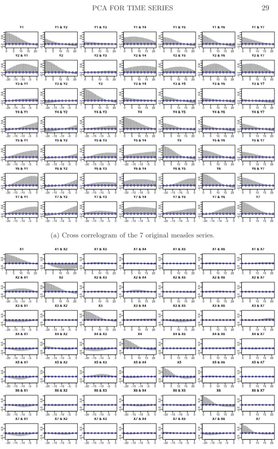
Example2. We consider the weekly notified measles cases in 7 cities in
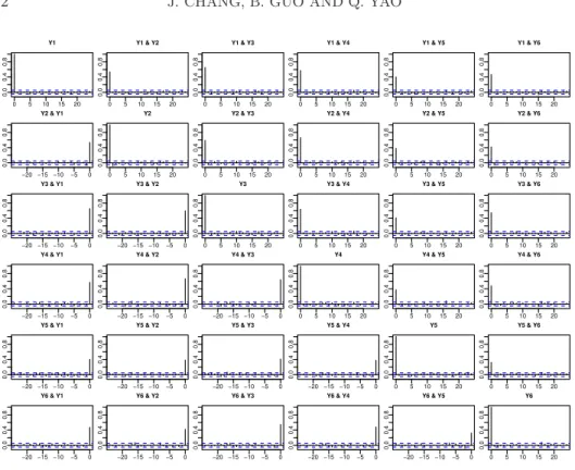
England (i.e. London, Bristol, Liverpool, Manchester, Newcastle, Birming-ham and Sheffield) in 1948 – 1965, before the advent of vaccination. All the 7 series show biennial cycles, which is a common feature in measles dynam-ics in the pre-vaccination period. This biennial cycling is the major driving force for the cross correlations among different component series displayed in Fig 2(a). The cross correlogram of the transformed data is displayed in Fig 2(b). Since none of the transformed component series are white noise, the confidence bounds in Fig 2(b) could be misleading; see Remark 1(i).
We apply prewhitening to each transformed component time series by fitting an AR model with the order determined by AIC. Although all those 7 filtered time series behave like white noise, there are still quite a few small but significant cross correlations here and there. Fig 3(a) plots, in descending
Table 1
One-step and two-step ahead post-sample forecasting: means and standard deviations (in subscripted bracket) of MSPEs for Examples 1, 3 and 4 and means and standard
deviations (in subscripted bracket) of the relative MSPEs for Example 2.
Method One-step forecast Two-step forecast VAR 2.470(0.416) 2.559(0.385)
Example 1 RVAR 2.530(0.398) 2.615(0.382)
(p=7) Segmentation with 5 groups 2.221(0.339) 2.203(0.323)
Segmentation with 6 groups 2.417(0.348) 2.419(0.326)
Segmentation with 4 groups 2.421(0.343) 2.422(0.325)
VAR 0.950(0.148) 0.726(0.328)
Example 2 RVAR 0.962(0.138) 0.796(0.277)
(p=7) Segmentation with 4 groups 0.884(0.180) 0.708(0.377)
Segmentation with 7 groups 0.919(0.130) 0.884(0.219)
Segmentation with 3 groups 0.873(0.176) 0.694(0.377)
Univariate AR 0.208(0.551) 0.194(0.539)
VAR 0.295(0.806) 0.301(0.855)
Example 3 RVAR 0.293(0.820) 0.296(0.863)
(p=25) Segmentation with 24 groups 0.153(0.134) 0.163(0.124)
Segmentation with 25 groups 0.110(0.084) 0.132(0.091)
Segmentation with 23 groups 0.151(0.133) 0.159(0.121)
Univariate AR 0.525(0.204) 0.835(0.284)
Example 4 Segmentation with 83 groups 0.485(0.185) 0.662(0.224)
(p=84) Segmentation with 84 groups 0.484(0.184) 0.662(0.224)
Segmentation with 50 groups 0.492(0.187) 0.678(0.228)
Segmentation with 70 groups 0.474(0.180) 0.664(0.225)
order, the maximum cross correlationsLbn(i, j) defined in (2.11) for those 7
transformed and prewhitened series. As 1.96/√n = 0.064 with n = 937 now, one may argue that the segmentation assumption does not hold for this example. Consequently the ratio estimatorrbdefined in (2.12) does not make any sense for this example; see also Fig 3(b).
Nevertheless Fig 3(a) ranks the pairs of transformed component series according to the strength of the cross correlation. If we would only accept r connected pairs, this leads to an approximate segmentation according to the rule set in Section 2.2.1. By doing this, we effectively ignore some small, though still statistically significant, cross correlations. Table 2 lists the dif-ferent segmentations corresponding to the difdif-ferent values ofr. It shows that the group{4, 5}is always present until all the 7 series merge together. Fur-ther it only takes 6 connected pairs, corresponding to the 6 largest points in Fig 3(a), to merge all the series together.
The forecasting comparison is conducted in the same manner as in Ex-amples 1. We adopt the segmentation with 4 groups: {1, 2, 3}, {4, 5}, {6} and {7}, i.e. we regard that only the three pairs, corresponding to the 3
Table 2
Segmentations determined by different numbers of connected pairs for the transformed series in Example 2.
No. of connected pairs No. of groups Segmentation
1 6 {4, 5},{1},{2},{3},{6},{7} 2 5 {1, 2},{4, 5},{3},{6},{7} 3 4 {1, 2, 3},{4, 5},{6},{7} 4 3 {1, 2, 3, 7},{4, 5},{6} 5 2 {1, 2, 3, 6, 7},{4, 5} 6 1 {1, . . . ,7}
maximum cross correlations in Fig 3(a), are connected. We forecast the no-tified measles cases in the last 14 weeks of the period for all the 7 cities. Due to the fact that the data from different cities are on different scales, we present the results based on relative MSPEs in Table 1: a relative MSPE is the ratio of a MSPE concerned over that obtained from fitting each original component series with an AR model. Once again the forecasting based on this (approximate) segmentation is much more accurate than those based on the direct VAR and RVAR models, although we have ignored quite a few small but significant cross correlations among the transformed series. Table 1 also reports an over-segmentation case with each transformed series as an individual group, and an alternative segmentation case with 3 groups ({1, 2, 3, 7},{4, 5},{6}). The over-segmentation ignores all the correlations among different components, it has an adverse effect on forecasting, though it still outperforms the VAR and RVAR models. The alternative segmenta-tion with the 3 groups takes into account more correlasegmenta-tions, leading to the best forecasting performance in comparison with the other methods.
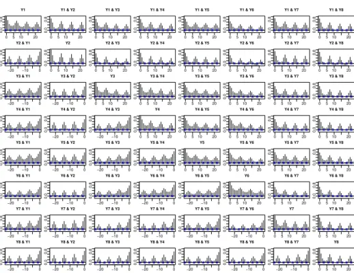
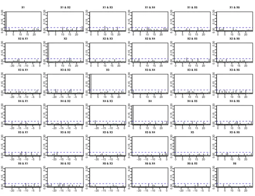
Example 3. Now we consider the daily log-sales of a clothing brand in
25 provinces in China in 1 January 2008 – 9 December 2012 (i.e.n= 1805 and p = 25). All those series exhibit peaks before the Spring Festival (i.e. the Chinese New Year, typically around February). The cross correlogram of the 8 randomly selected component series in Fig 4 indicates the strong cross correlations over different time lags among the sales over different provinces. The strong periodic components with the period 7 indicate a regular sales pattern over 7 different weekdays. By applying the proposed segmentation transformation and the permutation based on the maximum cross correlations with m = 25 in (2.11), the transformed 25 time series are divided into 24 group with only non-single-element group containing the 15th and the 16th transformed series. The same grouping is obtained form between 14 and 30. Note for this example, we should not use smallm as the
autocorrelations of the original data decay slowly; see Fig 4.
To compare the post-sample forecasting performance, we calculate one-step-ahead and two-one-step-ahead forecasts for each of the daily log-sales in the last two weeks of the period. Table 1 list the means and the standard deviations of the MSPEs across the 25 provinces. With p = 25, the fitted VAR(2) model, selected by AIC, contain 2×25×25 = 1250 parameters, leading to poor post-sample forecasting. The RVAR(2) model improves the forecasting a bit, but it is still significantly worse than the forecasting based on the approach of fitting a univariate AR model to each of the original series directly. Since the proposed segmentation leads to 24 subseries, it also fits univariate AR models to 23 (out of 25) transformed series, fits a 2-dimensional VAR model to the 15th and the 16th transformed series together. The proposed approach leads to much more accurate forecasts as both the mean and standard deviation are much smaller than those of the other three methods. The above comparison shows clearly that the cross correlations in the sales over different provinces are valuable information which can improve the forecasting for the future sales significantly. However the endeavor to reduce the dimension by, for example, TS-PCA, is necessary in order to make use of this valuable information. We also consider an over-segmentation by regarding each component of the transformed series as an individual group, and an incomplete-segmentation with{5, 15, 16}as a group and the other 22 components as 23 individual groups. Both of them show good performances.
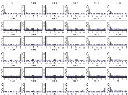
Example 4. The air pollution due to the fine particulate (PM2.5) has
aroused serious concerns in China. PM2.5 consists of airborne particles with
aerodynamic diameters smaller than 2.5µm. In this example, we consider the logarithmic daily average PM2.5 concentration readings at 84 monitoring
stations in Beijing, Tianjin and Hebei in 1 January 2015 – 31 December 2016. Fig 5 is a map of those 84 stations. For this data set, n = 731 and p= 84. The readings at different locations are crossly correlated; see Fig 6 for the cross-correlogram of six randomly selected stations.
Since the dimensionp is large, we use (3.5) to estimate the positive defi-nite matrixSbwith the threshold leveludetermined by the method of Bickel and Levina (2008). The maximum cross correlation method in Section 2.2.2 divides the 84 transformed time series into 83 groups, with only one non-single element group containing the 46th and the 83rd transformed series. In the post-sample forecasting for the daily readings in December 2016 (i.e. 31 days in total), we also include the over-segmentation with 84 groups (i.e. treating each transformed series as an individual group), and two incomplete
segmentations with, respectively, 50 groups and 70 groups. The maximum group size is 8 for the segmentation with 50 groups, and is 4 for the seg-mentation with 70 groups. Those segseg-mentations are obtained in the same manner as in Example 2 (see also Table 2). With p = 84, direct VAR is too crude to be attempted. Comparing to the univariate AR models for the original series, all the four segmentations provide more accurate one-step and two-step ahead predictions. It is worth pointing out that the difference due to using different segmentations is small.
5. Segmenting multivariate volatility processes. The methodol-ogy proposed in Section 2 can be readily extended to segment multivari-ate volatility processes. To this end, let yt be a p×1 volatility process.
Let Ft = σ(yt,yt−1, . . .) and Var(yt|Ft−1) = Σy(t). Without loss of
gen-erality, we assume E(yt|Ft−1) = 0 and Var(yt) = Ip. Suppose that there
exists an orthogonal matrix A for which yt = Axt and Var(xt|Ft−1) =
diag{Σ1(t), . . . ,Σq(t)}withΣ1(t), . . . ,Σq(t) being, respectively,p1×p1, . . . ,
pq×pqnon-negative definite matrices. Hence the latentp-dimensional
volatil-ity processxtcan be segmented intoqlower-dimensional processes, and there
exist noconditional cross correlations across those q processes. LetWy =PB∈Bt−1[E{yty
T
tI(B)}]2 and Wx =PB∈Bt−1[E{xtx
T
tI(B)}]2,
where Bt−1 is a π-class and the σ-field generated by Bt−1 equals to Ft−1.
Since it holds for anyB ∈ Bt−1thatE{xtxTtI(B)}=E{I(B)E(xtxTt|Ft−1)}=
E[I(B)diag{Σ1(t), . . . ,Σq(t)}] is a block diagonal matrix, so is Wx. Now
(2.6) still holds for the newly defined Wy and Wx. Thus A can be esti-mated exactly in the same manner as in Section 2.1. An estimator for Wy
can be defined asWcy =PB∈B
Pk0
k=1{(n−k)−1
Pn
t=k+1ytyTtI(yt−k ∈B)}2,
whereBis a set with elements{u∈Rp :kuk2 ≤ kytk2}fort= 1, . . . , n. See
Fan, Wang and Yao (2008). We illustrate this idea by a real data example.
Example5. We consider the daily returns of the stocks of Walt Disney
Company, Wells Fargo & Company, Honeywell International Inc., MetLife Inc., H & R Block Inc. and Cognizant Technology Solutions Corporation in 14 July 2008 – 11 July 2014. For this data set,n= 1509 andp= 6. Denote by yt = (y1,t, . . . , y6,t)T the returns on the t-th day. By fitting each return
series a GARCH(1,1) model, we calculate the residuals εi,t = yi,t/σbi,t for
i = 1, . . . ,6, where bσi,t denotes the predicted volatility for the i-th return
at timetbased on the fitted GARCH(1,1) model. The cross correlogram of the residual series are plotted in Fig 7(a), which shows the strong and sig-nificant concurrent correlations across all residual series. It indicates clearly that Var(yt|Ft−1) is not a block diagonal matrix. We also apply the
series is shown in Fig 7(b). There are also strong and significant concurrent correlations across the residual series, see Panels (1, 2), (2, 3), (3, 4), (2, 5) and (6, 4). This indicates all the principal components should not be mod-elled separately. Now we apply the segmentation transform stated above. We repeat the whitening process above for the transformed seriesxbt, i.e. fit an
GARCH(1,1) model for each of the component series ofxbtand calculate the
residuals. Fig 8 presents the cross correlogram of these new residual series. There exist almost no significant cross correlations among the residual series. This is the significant evidence to support the assertion that Var(xt|Ft−1) is
a diagonal matrix. For this example, the segmentation method leads to the conditional uncorrelated components of Fan, Wang and Yao (2008).
6. Final remarks. This paper proposes a contemporaneous linear trans-formation to segment a multiple time series into several both contempora-neously and serially uncorrelated subseries. The method is simple, and can be used as a preliminary step to reduce a high-dimensional time series mod-elling problem into several lower-dimensional problems. The reduction of dimensionality is often substantial and effective.
The method is abbreviated as TS-PCA, as it can be viewed as a version of PCA for multiple time series. Like the standard PCA, TS-PCA techni-cally also boils down to an eigenanalysis for a positive definite matrix. The difference is that the intended segmentation is not guaranteed to exist. How-ever one of the strengths of the proposed TS-PCA is that even when the segmentation assumption is invalid, it provides some approximate segmen-tations which ignore some minor (though still significant) cross correlations and, thus, lead to parsimonious modelling strategies. Those parsimonious strategies often bring in improvements in, for example, forecasting future values. See, e.g., Example 2. Furthermore when the dimension of time se-ries is large, TS-PCA is necessary in order to utilize the information across different component series effectively. See, e.g., Examples 3 and 4.
We have conducted some post-sample forecasting comparison with several real data sets including some not reported in the paper. The forecasting based on the proposed TS-PCA always outperforms that for the original data. We give one explanation as follows. It follows from (2.6) that Ω ≡ tr(Wy)−p = Pkk0=1
Pp
i,j=1ρ2y,ij(k) = tr(Wx)−p = Pkk0=1
Pp
i,j=1ρ2x,ij(k),
whereρy,ij(k) and ρx,ij(k) denote, respectively, the cross correlation at lag
k between the i-th and the j-th components of yt and xt. Since the future
prediction is based on the serial correlations, Ω can be taken as a measure for the predictive strength, which is the same for yt and xt. To make use
appropriately to catch all the autocorrelations and cross-correlations (over different time lags) among thepcomponents of yt. In contrast, such a task
forxtis much easier as it can be divided intoqlower-dimensional problems.
In the ideal situation when q = p, i.e. ρx,ij(k) = 0 for any i 6= j, we just
need to model all the component series ofxtseparatelyin order to make the
full use of the overall predictive strength.
Acknowledgements. The authors sincerely thank the Co-Editor, As-sociate Editor and three referees for their constructive suggestions and com-ments that led to substantial improvement of the paper.
References.
Anderson, T. W. (1963). The use of factor analysis in the statistical analysis of multiple time series.Psychometrika,28, 1–25.
Back, A. D. and Weigend, A. S. (1997). A first application of independent component analysis to extracting structure from stock returns.Int. J. Neural Syst.,8, 473–484. Bai, J. and Ng, S. (2002). Determining the number of factors in approximate factor models.
Econometrica, 70, 191–221.
Belouchrani, A., Abed-Meraim, K., Cardoso, J.-F. and Moulines, E. (1997). A blind source separation technique using second-order statistics.IEEE T. Signal Proces.,45, 434–444. Bickel, P. J. and Levina, E. (2008). Covariance regularization by thresholding.Ann. Stat.,
36, 2577–2604.
Box, G. E. P. and Jenkins, G. M. (1970).Time Series Analysis, Forecasting and Control.
Holden-Day, San Francisco.
Box, G. E. P. and Tiao, G. C. (1977). A canonical analysis of multiple time series.
Biometrika,64, 355–365.
Brockwell, P. J. and Davis, R. A. (1996). Introduction to Time Series and Forecasting. Springer, New York.
Brillinger, D. R. (1981). Time Series: Data Analysis and Theory. Holt, Rinehart and Winston, New York.
Cardoso, J. (1998). Multidimensional independent component analysis.Proceedings of the
1998 IEEE Int. Conf. Acoustics, Speech and Signal Processing,4, 1941–1944.
Chang, J., Guo, B. and Yao, Q. (2015). High dimensional stochastic regression with latent factors, endogeneity and nonlinearity.J. Econometrics,189, 297–312.
Chang, J., Guo, B. and Yao, Q. (2017). Supplement to “Principal component analysis for second-order stationary vector time series.”
Testing for high-dimensional white noise using maximum cross correlations. Biometrika, in press.
Davis, R. A., Zang, P. and Zheng, T. (2012). Sparse vector autoregressive modelling. Available atarXiv:1207.0520.
Fan, J., Wang, M. and Yao, Q. (2008). Modelling multivariate volatilities via conditionally uncorrelated components.J. Roy. Stat. Soc. B.,70, 679–702.
Fan, J. and Yao, Q. (2003).Nonlinear Time Series: Nonparametric and Parametric Meth-ods. Springer, New York.
Forni, M., Hallin, M., Lippi, M. and Reichlin, L. (2005). The generalized dynamic factor model: One-sided estimation and forecasting.J. Am. Stat. Assoc.,100, 830–840. Guo, S., Wang, Y. and Yao, Q. (2016). High-dimensional and banded vector
Han, F. and Liu, H. (2013). A direct estimation of high dimensional stationary vector autoregressions. Available atarXiv:1307.0293.
Huang, D. and Tsay, R. S. (2014). A refined scalar component approach to multivariate time series modeling.Manuscript.
Hyv¨arinen, A., Karhunen, J. and Oja, E. (2001).Independent Component Analysis. Wiley, New York.
Jakeman, A. J., Steele, L. P. and Young, P. C. (1980). Instrumental variable algorithms for multiple input systems described by multiple transfer functions. IEEE T. Syst. Man. Cyb.,10, 593–602.
Lam, C., Yao, Q. and Bathia, N. (2011). Estimation of latent factors for high-dimensional time series.Biometrika,98, 901–918.
Lam, C. and Yao, Q. (2012). Factor modeling for high-dimensional time series: inference for the number of factors.Ann. Stat.,40, 694–726.
Ledoit, O. and Wolf, M. (2004). A well-conditioned estimator for large-dimensional co-variance matrices.J. Multivariate Anal.,88, 356–411.
Liu, W., Xiao, H. and Wu, W. B. (2013). Probability and moment inequalities under dependence.Statist. Sinica,23, 1257–1272
L¨utkepohl, H. (2006).New Introduction to Multiple Time Series Analysis. Springer, Berlin. Matteson, D. S. and Tsay, R. S. (2011). Dynamic orthogonal components for multivariate
time series.J. Am. Stat. Assoc.,106, 1450–1463.
Pan, J. and Yao, Q. (2008). Modelling multiple time series via common factors.Biometrika, 95, 365–379.
Paparoditis and Politis (2012). Nonlinear spectral density estimation: thresholding the correlogram.J. Time Ser. Anal.,33, 386–397.
Pe˜na, D. and Box, G. E. P. (1987). Identifying a simplifying structure in time series.J.
Am. Stat. Assoc.,82, 836–843.
Reinsel, G. C. (1993). Elements of Multivariate Time Series Analysis (2nd edition). Springer.
Rio, E. (2000). Th´eorie asymptotique des processus al´eatoires faiblement d´ependants. Springer, Berlin.
Sarkar, S. K. and Chang, C.-K. (1997). The Simes method for multiple hypothesis testing with positively dependent test statistics.J. Am. Stat. Assoc.,92, 1601–1608.
Shojaie, A. and Michailidis, G. (2010). Discovering graphical Granger causality using the truncated lasso penalty.Bioinformatics,26, 517–523.
Simes, R. J. (1986). An improved Bonferroni procedure for multiple tests of significance.
Biometrika,73, 751–754.
Song, S. and Bickel, P. J. (2011). Large vector auto regressions. Available at
arXiv:1106.3519.
Stewart, G. W. and Sun, J. (1990).Matrix Perturbation Theory. Academic Press. Stock, J. H. and Watson, M. W. (2002), Forecasting using principal components from a
large number of predictors.J. Am. Stat. Assoc.,97, 1167–1179.
Stock, J. H. and Watson, M. W. (2005). Implications of dynamic factor models for VAR analysis. Available atwww.nber.org/papers/w11467.
Theis, F. J., Meyer-Baese, A. and Lang, E. W. (2004). Second-order blind source separation based on multi-dimensional autocovariances. InIndependent Component Analysis and
Blind Signal Separation(Edi. C.G. Puntonet and A. Prieto). Springer, 726-733.
Tiao, G. C. and Tsay, R. S. (1989). Model specification in multivariate time series (with discussion).J. Roy. Stat. Soc. B.,51, 157–213.
Tong, L. Xu, G. and Kailath, T. (1994). Blind identification and equalization based on second-order statistics: a time domain approach.IEEE T. Inform. Theory,40, 340–349.
Tsay, R. (2014).Multivariate Time Series Analysis. Wiley.
Center of Statistical Research and
School of Statistics
Southwestern University of Finance and Economics
Chengdu, Sichuan 611130 China
E-mail:[email protected];[email protected]
Department of Statistics London School of Economics
and Political Science London, WC2A 2AE UK