Rochester Institute of Technology
RIT Scholar Works
Theses
3-2018
Control of PV Connected Power Grid using LQR
and Fuzzy Logic Control
Samar Emara
Follow this and additional works at:https://scholarworks.rit.edu/theses
This Thesis is brought to you for free and open access by RIT Scholar Works. It has been accepted for inclusion in Theses by an authorized administrator of RIT Scholar Works. For more information, please [email protected].
Recommended Citation
Control of PV Connected Power Grid using LQR
and Fuzzy Logic Control
by
Samar Emara
A Thesis Submitted in Partial Fulfillment of the
Requirements for the Degree of Master of Science in Electrical Engineering
Department of Electrical Engineering and Computing Sciences
Rochester Institute of Technology, Dubai UAE
ii
Control of PV Connected Power Grid using LQR and
Fuzzy Logic Control
by
Samar Emara
A Thesis Submitted in Partial Fulfilment of the Requirements for the Degree of Master of Science in Electrical Engineering Department of Electrical Engineering and Computing Sciences
Approved By:
_____________________________________________Date:______________ Dr. Abdulla Ismail
Thesis Advisor – Department of Electrical Engineering
_____________________________________________Date:______________ Dr. Yousef Al Assaf
Committee Member – Department of Electrical Engineering
_____________________________________________Date:______________ Dr. Ghalib Kahwaji
iii
Acknowledgements
I would like to express my sincere gratitude to Dr. Abdulla Ismail, the advisor of this thesis,
for his continuous support and guidance. Without him the completion of this research
would not have been possible. His door was always open to help me in my thesis and I am
honored to have him as my thesis advisor.
I would also like to thank Dr. Ali Sayyad for his helpful guidance and valuable comments
on my thesis work and for all the time he dedicated to help me. Many thanks also to my
colleagues at RIT Dubai and my professors for their support and encouragement.
My sincere thanks and appreciation to Dr. Yousef Al Assaf, president of RIT Dubai and
Dr. Ghalib Kahwaji, head of the Mechanical Engineering at RIT Dubai, for giving me from
their time to read and evaluate this thesis.
Last but not least, I would like to deeply thank my parents for their continuous support and
encouragement throughout this journey. Their support always leads me to success and
iv
v
Abstract
As the contribution of renewable energy to the current power grid is becoming an
essential part of the global energy system, it is of critical importance to study the effects of
this increased penetration of the renewable sources on the power system. Focusing on solar
energy, its intermittent nature makes it difficult to predict the output when connecting to
the power grid. Therefore, well-structured control methods should be used to assure a
continuous and steady system performance with regard to the system frequency variation.
In this thesis, a PV system is modelled and connected to a grid served by a
conventional thermal power system with 45% penetration level. Then, the system
frequency errors due to load changes are studied in this PV connected power grid.
Appropriate and effective controllers are designed to regulate these errors to keep the
system response within the required specifications.
In addition, single-area as well as two-area interconnected power systems are
considered in this research. The power exchange among the two areas will add another
significant parameter that is essential in the efficient operation of the system and that
affects the behavior of the system in terms of the frequency error response.
Two advanced control methods, namely Linear Quadratic Regulator (LQR) and
Fuzzy Logic Control (FLC) are applied to control the single-area and the two-area systems.
The appropriate controllers are designed, assessed and the responses are analyzed and
compared. These designed controllers demonstrated a superior performance in the
controlled system by achieving the required specifications of undershoot, settling time and
steady state error for the system frequency. For the single-area PV connected power
system, the LQR controller gave the best response in comparison to the two other types of
controllers, while in the two-area system the fuzzy logic controller was the most suitable
vi
Table of Contents
Acknowledgements ... iii
Abstract ... v
List of Figures ... viii
List of Tables ... xii
List of Main Symbols... xiv
List of Main Abbreviations ... xv
List of Publications ... xvi
Chapter 1: Introduction ... 1
1.1 Research Motivation ... 1
1.2 Research Objectives ... 3
1.3 Thesis Organization... 3
Chapter 2: Literature Review... 5
2.1 Photovoltaic Systems ... 5
2.2 Thermal Power System ... 8
2.3 Linear Quadratic Regulators ... 11
2.4 Fuzzy Logic Controllers ... 13
Chapter 3: Uncontrolled System Modeling ... 18
3.1 Model of the Photovoltaic System ... 18
3.2 Thermal Power System – Single Area ... 31
3.3 Model of the PV System Connected to the Single-Area Power Grid ... 36
3.4 Model of the Two-Area Power Grid Connected to the PV System ... 42
Chapter 4: Controller Design and Analysis ... 51
4.1 Design of the Linear Quadratic Regulation for PV Grid-Connected Single-Area Power Grid ... 51
4.1.1 Case 1: Acceptable increase in load (∆𝑷𝒍𝒐𝒂𝒅 < 𝟏𝟎%) ... 52
4.1.2 Case 2: 50% increase in load (worst-case scenario) ... 53
4.2 Design of PI Controller for PV Grid-Connected Single-Area Power Grid ... 55
4.2.1 Case 1: Acceptable increase in load (∆𝑷𝒍𝒐𝒂𝒅 < 𝟏𝟎%) ... 55
vii
4.3 Design of Fuzzy Logic Controller for PV Grid-Connected Single-Area Power Grid 57
4.3.1 Case 1: Acceptable increase in load (∆𝑷𝒍𝒐𝒂𝒅 < 𝟏𝟎%) ... 63
4.3.2 Case 2: 50% increase in load (worst-case scenario) ... 64
4.4 Design of the Linear Quadratic Regulation for PV Grid-Connected Two-Area Power Grid ... 66
4.4.1 Case 1: Acceptable increase in load (∆𝑷𝒍𝒐𝒂𝒅𝟏 = ∆𝑷𝒍𝒐𝒂𝒅𝟐) ... 67
4.4.2 Case 2: ∆𝑷𝒍𝒐𝒂𝒅𝟏 > ∆𝑷𝒍𝒐𝒂𝒅𝟐 ... 68
4.4.3 Case 3: ∆𝑷𝒍𝒐𝒂𝒅𝟐 > ∆𝑷𝒍𝒐𝒂𝒅𝟏 ... 69
4.4.4 Case 4: ∆𝑷𝒍𝒐𝒂𝒅𝟏 = ∆𝑷𝒍𝒐𝒂𝒅𝟐 = 𝟓𝟎% (worst-case scenario) ... 71
4.5 Design of PI Controller for PV Grid-Connected Two-Area Power Grid ... 72
4.5.1 Case 1: Acceptable increase in load (∆𝑷𝒍𝒐𝒂𝒅𝟏 = ∆𝑷𝒍𝒐𝒂𝒅𝟐) ... 74
4.5.2 Case 2: ∆𝑷𝒍𝒐𝒂𝒅𝟏 > ∆𝑷𝒍𝒐𝒂𝒅𝟐 ... 76
4.5.3 Case 3: ∆𝑷𝒍𝒐𝒂𝒅𝟐 > ∆𝑷𝒍𝒐𝒂𝒅𝟏 ... 78
4.5.4 Case 4: ∆𝑷𝒍𝒐𝒂𝒅𝟏 = ∆𝑷𝒍𝒐𝒂𝒅𝟐 = 𝟓𝟎% (worst-case scenario) ... 80
4.6 Design of Fuzzy Logic Controller for PV Grid-Connected Two-Area Power Grid 82 4.6.1 Case 1: Acceptable increase in load (∆𝑷𝒍𝒐𝒂𝒅𝟏 = ∆𝑷𝒍𝒐𝒂𝒅𝟐) ... 84
4.6.2 Case 2: ∆𝑷𝒍𝒐𝒂𝒅𝟏 > ∆𝑷𝒍𝒐𝒂𝒅𝟐 ... 86
4.6.3 Case 3: ∆𝑷𝒍𝒐𝒂𝒅𝟐 > ∆𝑷𝒍𝒐𝒂𝒅𝟏 ... 88
4.6.4 Case 4: ∆𝑷𝒍𝒐𝒂𝒅𝟏 = ∆𝑷𝒍𝒐𝒂𝒅𝟐 = 𝟓𝟎% (worst-case scenario) ... 90
Chapter 5: Analysis & Conclusion ... 93
5.1 PV Grid Connected Single-Area Analysis ... 93
5.2 PV Grid Connected Two-Area Analysis ... 96
5.3 Conclusions and Further Works ... 99
References ... 101
viii
List of Figures
Figure 1.1 a PV system connected to the load in the grid directly [6]. ... 2
Figure 2.1 Stages of connection of PV array output to the three-phase power grid [15]. .. 6
Figure 2.2 IV characteristics of PV array showing the point at which MPP occurs [14]. .. 7
Figure 2.3 Changes of load demand and PV input throughout a day in a residential application. ... 8
Figure 2.4 General diagram of the main components of a single-area thermal power system. ... 9
Figure 2.5 Load frequency control mechanism [23]. ... 10
Figure 2.6 Difference between min and max operators for fuzzy inference stage. ... 14
Figure 2.7 Example of a triangular shape of a membership function in a fuzzy set. ... 14
Figure 2.8 General fuzzy logic controller design stages. ... 15
Figure 2.9 Example of two rules obtained from inference mechanism. ... 16
Figure 3.1 General mathematical model of the connection between the PV array and the grid. ... 19
Figure 3.2 Current Inversion from DC (after boost converter) to AC with 50Hz (system frequency). ... 21
Figure 3.3 Instantaneous power from the photovoltaic system (100 Hz). ... 22
Figure 3.4 Average power output of the PV (second input to conventional power system). ... 24
Figure 3.5 PV system designed model. ... 24
Figure 3.6 DC-AC inverter block to obtain controllable canonical form. ... 25
Figure 3.7 Instantaneous power blocks to obtain controllable canonical form. ... 26
Figure 3.8 Average power block to obtain controllable canonical form. ... 27
Figure 3.9 The full PV system model from which the controllable canonical form was obtained. ... 30
Figure 3.10 Block diagram of the single-area thermal power system without any controller. ... 31
Figure 3.11 Response of the single-area thermal power system due to a 50% increase in load without any controller. ... 32
Figure 3.12 Block diagram of the single-area thermal power system with integral controller only. ... 33
Figure 3.13 Single-area thermal power system frequency error response to a 50% increase in load (with integral controller only). ... 35
Figure 3.14 Power generated mechanically from the thermal system to match 50% increase of load in the system with integral controller only. ... 36
Figure 3.15 The photovoltaic system connected to the grid. ... 38
Figure 3.16 Comparison between responses of the system connected and unconnected to the PV system (100% load increase). ... 39
ix
Figure 3.18 Response of the system with and without PV (for a reasonable change in load). ... 40 Figure 3.19 thermal power system provides the remaining power that the PV system could not provide. ... 42 Figure 3.20 Block diagram of the second area. ... 42 Figure 3.21 The response of the second area only with integral controller. ... 44 Figure 3.22 Response of the two-area system without any controller due to 50% increase in load... 46 Figure 3.23 Block diagram of the two-area system with PV connected to the grid (I controller only)... 48 Figure 3.24 Change of frequency from area 1 and area 2 (for the system only with
integral controller) for reasonable load. ... 49 Figure 3.25 Change of frequency from area 1 and area 2 (for the system only with
x
Figure 4.17 Response of both areas with LQR controller for equal change in load of 50%. ... 71 Figure 4.18 Two-area system with PI controller. ... 73 Figure 4.19 Response of area 1 in the two-area system for a reasonable increase in load. ... 74 Figure 4.20 Response of area 2 in the two-area system for a reasonable increase in load. ... 75 Figure 4.21 Tie-line power change response due to a reasonable increase in load. ... 75 Figure 4.22 Response of area 1 in the two-area system due to more increase in load in area 1 than in area 2. ... 76 Figure 4.23 Response of area 2 in the two-area system due to more increase in load in area 1 than in area 2. ... 77 Figure 4.24 Tie-line power change between area 1 and 2 area 2 for more increase in load in area 1 than in area 2. ... 77 Figure 4.25 Response of area 1 in the two-area system due to more increase in load in area 2 than in area 1. ... 78 Figure 4.26 Response of area 2 in the two-area system due to more increase in load in area 2 than in area 1. ... 79 Figure 4.27 Tie-line power change between area 1 and area 2 due to more increase in load in area 1 than in area 2. ... 79 Figure 4.28 Response of area 1 in the two-area system for a 50% increase in load. ... 80 Figure 4.29 Response of area 2 in the two-area system for a 50% increase in load. ... 81 Figure 4.30 Tie-line power change between area 1 and area 2 for a 50% increase in load. ... 81 Figure 4.31 Two-area system with PI and FLC. ... 83 Figure 4.32 Response of area 1 with PI and fuzzy logic controllers for equal and
reasonable change in load. ... 84 Figure 4.33 Response of area 2 with PI and fuzzy logic controllers for equal and
xi
xii
List of Tables
Table 3.1 Parameters of the thermal power system. ... 31 Table 3.2 Response summary due to a 50% increase in load. ... 32 Table 3.3 Response summary of the single-area thermal power system for a 50% increase in load... 35 Table 3.4 Comparison for the different responses of the thermal power system connected and unconnected to the PV system. ... 40 Table 3.5 Parameters for the modeling of the second area in the thermal power system. 43 Table 3.6 Summary of the response of the second area only with integral controller. ... 44 Table 3.7 Response specifications summary of the two-area system without any
controller due to 50% increase in load. ... 47 Table 3.8 Summary of the response of both changes in frequency of the two-area system for 50% load. ... 50 Table 4.1 Response characteristics of the single-area system connected to PV with LQR controller (for reasonable load change). ... 53 Table 4.2 Response characteristics of PV-connected single-area system with LQR
xiii
xiv
List of Main Symbols
∆𝑓 Deviation of system frequency from 50Hz
∆𝑃𝑙𝑜𝑎𝑑 Change of load power
∆𝑃 Reference power
∆𝑃𝑝𝑣 Change of the photovoltaic system output power (input to thermal power system)
∆𝑃𝑡𝑖𝑒 Excess of scheduled power exchange between area 1 and area 2 in the power system
𝐴 System state matrix
𝑄 State Weighted Matrix in LQR controller
𝑅 Control Weighted Matrix in LQR controller
𝑃 Costate matrix in the Riccati equation
𝐾 Optimal state feedback gains in LQR
𝜇 Membership function
𝑘𝑖 Integral controller gain
𝑘𝑝 Proportional controller gain
∆𝑃𝑚 Turbine mechanical power
𝑒 Error
𝑒̇ Derivative of error
𝑢 Controller output
𝑉1 Output voltage from the PV array (V)
𝑉2 Voltage after the DC-DC boost converter (compatible with the grid voltage) (V)
𝑚 The gain between the DC voltage and the AC voltage in the system
𝑀1 Boost converter gain
𝐼1 Output current from the PV array (amp)
𝐼2 Current after the DC-DC boost converter in the PV system (amp)
𝑖𝐴𝐶 The inverted current in the PV system (amp)
𝑝 Instantaneous power of the PV system (W)
𝑃𝑎𝑣𝑔 Average power of the PV system (W)
𝑉𝑚 Phase grid voltage (V)
xv
List of Main Abbreviations
PV Photovoltaic
FLC Fuzzy Logic Controller
PI Proportional and Integral Controller
LQR Linear Quadratic Regulator
LFC Load Frequency Control
MPPT Maximum Power Point Tracking
MPP Maximum Power Point
SSE Steady State Error
p.u. Per unit system
NB Negative Big
NM Negative Medium
NS Negative Small
ZZ Zero change
PS Positive Small
PM Positive Medium
xvi
List of Publications
1- S. Emara and A. Ismail, “Design of fuzzy logic controller for a PV grid connected two-area load frequency control system,” International Research Journal of Engineering and Technology (IRJET), Vol. 05, issue: 02, February 2018.
2- S. Emara, A. Ismail and A. Sayyad, “Mathematical model of a photovoltaic grid connected two-area power system,” International Research Journal of Engineering and Technology (IRJET), Vol. 05, issue: 02, February 2018.
3- S. Emara, A. Ismail and A. Sayyad, “Optimal controller of a PV grid connected two-area power system,” International Research Journal of Engineering and Technology (IRJET), Vol. 05, issue: 02, February 2018.
1
Chapter 1:
Introduction
This chapter explains the motivation behind choosing the current research topic as
well as some general information concerning its importance. In addition, it explains the
detailed objectives of this research that will be focused on throughout the thesis. Finally,
the organization of the thesis report is explained for each of the subsequent chapters and
associated sections.
1.1
Research Motivation
It is estimated that more than 14% of the supply of the energy nowadays is from
renewable energy sources. However, there are always challenges to their implementation
because they have to meet certain requirements of voltage and frequency regulations in
order to be connected smoothly with the current power systems [1].
Many papers have studied PV connected grids and showed the direct connection of
PV to the load [2]. Those studies do not show the connection with the actual model of the
conventional power system as shown in Figure 1.1.
Control system design research has been conducted on performance enhancement
of isolated photovoltaic systems. Similarly, other works have been reported with regard to
the photovoltaic (PV) connected grid [3,4]. However, very few research has been
conducted on the effect of this interconnection on the system frequency and voltage
profiles. Moreover, some research has been conducted on the solar thermal power plant [5]
connected to the conventional power system and its effect on the system frequency
2
Figure 1.1 a PV system connected to the load in the grid directly [6].
It has been shown in some work that the penetration of renewable energy has an
effect on the system frequency and voltage [1]. Keeping the system frequency at an
acceptable constant level is a direct indicator of the power system real power and load
balance[7]. Therefore, the frequency change will be the main parameter of study in this
research. In order to achieve a high penetration level of PV, with its intermittent nature [8],
the operation and control of power systems need to account for the associated high
variability and uncertainty[9].
As PV is connected to the grid at the lower voltage side (for example, 11kV), thus,
the voltage imbalance is not of a lesser concern than the system frequency. Since there are
few papers that tackle the issue of frequency control in the PV connected grids with
explaining the full model of both the PV and the thermal power system, this was the main
3
1.2
Research Objectives
The objectives of this research can be summarized as follows:
1- Model a PV system that could properly be connected to a thermal power grid
and to model a single-area and two-area thermal power systems connected to it.
2- Design LQR, PI and FL controllers for a single-area and two-area power system
connected to the PV system with 45% penetration level.
3- Study the effect of load changes on the system frequency of a single-area and
two-area power system connected to PV.
4- Regulate the system frequency error ∆𝑓 by maintaining the following standard
performance specifications:
a. Settling time < 3s
b. Undershoot <0.02Hz
c. Steady state error of ∆𝑓 = 0
d. Steady state error of ∆𝑃𝑡𝑖𝑒 = 0 (for the two-area system)
When the power demand at the load side increases, it causes a drop of system
frequency. Since the reference frequency is 50Hz in the power grids in UAE, the tolerance
of this undershoot in frequency is 50Hz±0.02Hz. As to the steady state error of ∆𝑓 it
should equal zero implying that there is no change in frequency from the reference value
of 50Hz; i.e. 𝑓=50Hz. The exchange of power (∆𝑃𝑡𝑖𝑒) between areas will be explained
throughout the report.
1.3
Thesis Organization
Chapter 1 of this thesis explains the objectives of this research and the motivation
behind it. Chapter 2 shows the literature review of the recent relevant topics to this research.
Chapter 3 explains the mathematical model of the photovoltaic system, the single-area
thermal power system, the two-area thermal power system, and the connection between the
given PV system and the thermal power system.
Chapter 4 shows the designs of the three controllers (LQR, PI and FL controllers)
for the single-area and two-area PV grid connected systems. It shows several cases for each
4
and the power exchange between areas with these controllers integrated. In the last chapter,
the analysis of the responses of the controlled systems has been studied along with the
comparison between all controllers for different cases. The conclusion chapter summarizes
5
Chapter 2:
Literature Review
In this chapter, selected recent works on the subject are cited. The selected
information presented in this chapter explains the basic knowledge for each system that
will be studied and for each type of controller applied to these systems. This is essential in
the controller design stage, after studying the details of the systems and the controllers
design process.
2.1
Photovoltaic Systems
The smallest unit of a PV array is the solar cell, from which numerous arranged
solar cells are used to create a PV array. Based on knowledge of semiconductors physics,
a solar cell can be represented as a PN diode that produces DC current affected by the
changes of temperature, solar irradiance and the load [8]. The PN junction diode from
which a PV cell is created, has two different semiconductor elements; one that is doped
with excess positively charged holes (p-type) and another that is doped with excess
negatively charged electrons (n-type). The PN junction is the area that separates both sides
from each other and it is the area through which the current flows from the high intensity
of electrons (n-type) to the high intensity of holes (p-type). The sunlight excites more
electrons to move from the n-type to the p-type region creating the DC current which is the
output of the PV cell. Thus, this semiconductor structure takes the input and transforms it
into electric current by creating the PN junction described. This makes the output current
moves only in one direction (from the high intensity of electrons to the high intensity of
holes) [10].
Due to the DC output nature of the PV cell, it adds no kinetic energy to the system
[11]. Equations 2.1 and 2.2 describe the current produced from a single cell obtained from
the ideal PV cell based on semiconductor physics [12].
𝐼 = 𝐼𝑝𝑣,𝑐𝑒𝑙𝑙−
𝐼𝑜,𝑐𝑒𝑙𝑙[exp (∝ 𝐾𝑇) − 1]𝑞𝑉
𝐼𝑑
6 𝐼𝑑 = 𝐼𝑜,𝑐𝑒𝑙𝑙{exp [𝑞𝑉
𝐴 × 𝑘 × 𝑇] − 1}
𝐼 is the output current of the cell, 𝐼𝑝𝑣,𝑐𝑒𝑙𝑙 is the current generated by the incident
light of the sun on the cell, 𝐼𝑑 is the diode current since the PV cell operates as a diode and
𝐼𝑜,𝑐𝑒𝑙𝑙 is the diode reverse saturation value. 𝑉 is the output voltage, 𝐴 is the area of the
junction, 𝑇 is the temperature at the current time and 𝑞 and 𝑘 are constants determined
from the specifications of the PN junction diode.
In order to connect the PV array to a power grid, power electronics and devices are
required in the connection [13]. After obtaining the power output from the array, the first
stage of this connection with the thermal power grid is the boost converter. It increases the
voltage to a suitable level to be used as an input to the second stage which is the inverter.
The inverter produces an AC current which should be compatible with the AC nature of
the power grid. This requires compatibility with the grid voltage and current [14].
Capacitors are used to absorb the harmonics that are not desired of the low frequency
current [15]. Figure 2.1 shows the different stages of this connection. The output of the
inverter in Figure 2.1 is the input to the thermal power grid from the PV system.
Figure 2.1 Stages of connection of PV array output to the three-phase power grid [15].
As to the effect of this connection of PV to the thermal power system, it has been
shown in [16] and [17] that the more the penetration of the photovoltaic array output to the
conventional power grid, the less the deviation of the frequency output. In [8], it is
7
affect the frequency negatively at the transmission level, not at the utility grid side.
Therefore, the effect of PV connection to the grid has a positive effect on the frequency
which will be explained further in this work.
Nevertheless, the frequency still needs to be controlled to meet the required
specifications. The source in the PV arrays (which is the sun) cannot be controlled unlike
the conventional power systems where the amount of fluid can be controlled based on the
demand [18]. However, control can be performed in the photovoltaic system connection to
the grid in the DC-AC inverters [19]. It increases the efficiency of the system and ensures
the operation at Maximum Power Point (MPP). This is the point at which the maximum
output power is obtained. It occurs only at a certain voltage value; therefore, the output
voltage tracks the MPP in PV cells [19]. The Maximum Power Point Tracker (MPPT) is
the controller that tracks the maximum power point and ensures that the system operates at
this point most of the time [10].
This MPP occurs, as shown in Figure 2.2, when the slope of the load resistance
connected at the output of the PV array side happens to be the diagonal of the largest
rectangle that could be drawn on the IV characteristics curve of the PV array.
8
Another control possibility in the PV system is the following case. When the input
to the grid due to PV is more than the load demand at a certain point, power is inverted and
is injected back to the AC side. The photovoltaic system can be controlled if there is a
battery connected to it to improve the frequency control of the grid system [11].
Figure 2.3 shows actual data of the changes of the PV input along with the changes
in load throughout a day [20]. It can be seen that the peak of load demand happens in the
solar noon when the PV input is also at its maximum. PV input is minimum after 6pm, then
load starts decreasing after a while from that time as well. The part of the day studied in
this thesis is in the time when PV is at its maximum.
Figure 2.3 Changes of load demand and PV input throughout a day in a residential application.
2.2
Thermal Power System
The general block diagram of a single-area thermal power system is shown in
Figure 2.4 in which ∆𝑃 represents the speed changer (input to the system), ∆𝑃𝑙𝑜𝑎𝑑 represents a disturbance in the form of load power changes, and ∆𝑓 represents the deviation
of the system frequency from the nominal frequency value (50Hz). The first component in
this block diagram (the governor) is used to monitor and measure the system speed changes
and to control the valve. The turbine is the component that transforms the input energy (in
9
generator which will transform this mechanical energy into electrical energy. The reheater
makes the system more efficient as it reheats the steam to keep the same high temperature
of the steam that entered the governor [21]. The generator transforms the mechanical
energy into the electrical energy required.
Figure 2.4 General diagram of the main components of a single-area thermal power system.
The control of this thermal power system is conducted through a standard
generation called Automatic Generation Control (AGC) consists of two control loops:
Automatic Voltage Regulator (AVR) and Load Frequency Control (LFC) [22]. The focus
of this thesis is on the LFC to regulate the system frequency due to load demand changes.
When the load increases, the generator becomes slower [23]. This is because more power
is required to keep up with the same frequency level. Also, the generator in thermal power
system cannot go beyond a certain rated speed which limits the standard system frequency
to 50Hz. Therefore, when the load increases, the generator speed slows down and the
resulting frequency decreases [24]. This drop in frequency is not desired, and an
appropriate controller should be used to help the system retrieve its nominal frequency of
50Hz. This matching of the load should be performed as quickly as possible and with
minimal undershoot. No matter how much the load changes, the system should maintain a
frequency of 50Hz with minimal fluctuations. This is done by manipulating the fuel inlet
10
Figure 2.5 Load frequency control mechanism [23].
This valve operation is controlled primarily through Speed Regulation or Droop
(R). A droop is defined as the ratio between the changes in the frequency (∆𝑓) and the
change in the output power of the generator (∆𝑃𝐺) [22]. For instance, a value of 5% for the
speed regulation or droop implies that when the frequency deviates by 5%, it will cause a
100% change in the output power of the generator, i.e. a 100% change in the position of
the valve. The higher the droop, the better the regulation [23].
This droop is the primary control action for the system [11]. However, the response
due to the droop only is not sufficient as will be shown later. More reliable controllers are
needed to regulate the system frequency within the required limits of the settling time and
the undershoot.
As to the two-area system; where two separate power systems are interconnected,
the same concept applies with the addition of having tie-line power exchange (∆𝑃𝑡𝑖𝑒). The
tie-line is the transmission line that carries power between the two areas [21]. The excess
of power exchange of the tie-line between the two areas should also have a zero steady
state error when a load disturbance occurs [23]. When this change in the tie-line power is
zero, it implies that there is no excess power interchange between areas than the amount
scheduled between the two areas.
The frequency bias (𝑏𝑖) is also another parameter that is associated with the
two-area system rather than single-two-area. When a disturbance occurs (change in load power), the
11
Area Control Error (ACE) represents the accumulative error of both the frequency error
and the power exchange between both areas, while considering the effect of this frequency
bias [17]. The value of ACE should be kept zero or at a value very close to zero all the time
[25].
2.3
Linear Quadratic Regulators
The Linear Quadratic Regulator (LQR) is a standard optimal control technique. To
design an optimal controller, a performance measure should be chosen, which is the
objective that is required to be minimized or maximized by the optimal controller [26].
A certain state trajectory is defined after applying the controller signal obtained
from the optimal controller over a certain period of time along with an initial state for the
system at 𝑡0. The optimal control problem is defined as finding an optimal control 𝑢∗ for
the system in (2.3).
𝑥̇(𝑡) = 𝑓(𝑥(𝑡), 𝑢(𝑡), 𝑡)
which makes it follow an optimal trajectory 𝑥∗ that minimizes or maximizes the targeted
performance measure 𝐽 given in Equation 2.4 where ℎ and 𝑔 are scalar functions.
𝐽 = ℎ(𝑥𝑡𝑓, 𝑡𝑓) + ∫ 𝑔(𝑥(𝑡), 𝑢(𝑡), 𝑡)
𝑡𝑓
𝑡0
= 1
2[𝑧(𝑡𝑓) − 𝑦(𝑡𝑓)]
′
𝐹(𝑡𝑓)[𝑧(𝑡𝑓) − 𝑦(𝑡𝑓)]
+1
2∫ {[𝑧(𝑡) − 𝑦(𝑡)]
′𝑄(𝑡)[𝑧(𝑡) − 𝑦(𝑡)] + 𝑢′(𝑡)𝑅(𝑡)𝑢(𝑡)}𝑑𝑡 𝑡𝑓
𝑡𝑜
z(t) represents the desired output vector and y(t) represents the output vector. Q and
R are the matrices that should be chosen in order to give the minimum value of the
performance index (𝐽). Q is the error weighted matrix, and it should be positive
semidefinite. The more focus is required on minimizing a certain parameter, the larger the
weight that should be attributed to its corresponding state variable in the Q matrix. R is the
control weighted matrix and it should be positive definite [26]. At the final time (𝑡𝑓), the
terminal cost term (𝐹(𝑡𝑓)) should be 0, therefore, the first term of Equation 2.4 is cancelled. (2.3)
12
When the optimal values of Q and R matrices are substituted in the Riccati equation
(Equation 2.5), it provides the optimal costate matrix (P) [27].
𝑃(𝑡)̇ + 𝑃(𝑡)𝐴(𝑡) + 𝐴′(𝑡)𝑃(𝑡) + 𝑄(𝑡) − 𝑃(𝑡)𝐵(𝑡)𝑅−1(𝑡)𝐵′(𝑡)𝑃(𝑡) = 0
This costate matrix (P) is substituted into the optimal controller 𝑢∗(𝑡) (Equation
2.6) in the form of state feedback gains (K), as follows.
𝑢∗(𝑡) = 𝑅−1(𝑡)𝐵′(𝑡)𝑃(𝑡)𝑥∗(𝑡) = −𝐾(𝑡)𝑥∗(𝑡)
The optimal controller is implemented by feeding back these gains to their corresponding
state variables to obtain the optimal response of the system.
An optimal controller does not always exist for every system. In order to check if
an optimal controller exists for the system under study, the controllability and observability
matrices have to be obtained. If both matrices have ranks that are equal to the rank of the
system state matrix A from the state space model of the system, then an optimal controller
can be designed for this system, and the system is controllable and observable [26]. This is
important to ensure that the inputs are accessible, thus, can be controlled, and the outputs
are accessible, thus, can be observed and feedback to the system for the controller to
operate properly. Thus, for all systems in this thesis, the controllability and observability
matrices have been checked.
If the system is controllable and observable, and an optimal controller exists for the
system, the main challenge remaining in LQR is a suitable choice of the Q and R matrices
that are chosen based on the user experience [27]. An algebraic approach has been proposed
to calculate Q and R systematically [28]. The idea behind this approach is to compare
between the actual and the desired characteristic equations of the system. The desired
characteristic equation can be obtained for second and third order systems easily because
it is pre-defined according to the specifications of undershoot and settling time required.
Then, the comparison with the actual characteristic equation (in terms of P matrix
elements) is possible, and the P matrix would be obtained. This would solve the Riccati
equation. Based on that, and with assuming a certain value for the R matrix, the Q matrix
can be obtained by calculation rather than assumption.
(2.5)
13
However, this method has been tried for the systems presented in this thesis but
could not yield reasonable results. This is because the method presented in [28] is for
second and third order systems. However, the desired characteristic equation for higher
order systems has no pre-defined standard formulas related to the specifications (settling
time and undershoot). They rather depend on the choice of the desired closed loop poles,
which by their turn depend on user experience. Moreover, not all the elements in the P
matrix can be obtained by the comparison of both equations leaving behind many variables
that need to be tuned based on trial and error for higher order systems, which leads to a
very high cost function most of the time. Therefore, the best way to design LQR based
controller for a higher order system is by creating an optimization code and tuning the
system manually according to optimization results, which has been implemented in this
thesis.
2.4
Fuzzy Logic Controllers
Zadeh was the first to introduce the concept of fuzzy logic in 1965, then the
controllers based on fuzzy logic were introduced by Mamdani in 1974 [29]. The concept
of fuzzy logic is based on a concept similar to that of the binary logic (0,1). However, in
the binary logic, any value can either be in a set (therefore, having a value of 1) or not in a
set (having a value of 0). Things in the binary logic are either black or white. But in fuzzy
logic, each value can be considered as a member of a set by a certain percentage (either a
low or a high percentage). Thus, the values in fuzzy logic have partial memberships in the
set [30]. For example, if a certain set denotes old people, then it would be difficult to give
values of 0 and 1 for people who fit or do not fit strictly in this category. Fuzzy logic gives
the flexibility of assigning percentages to how much each person belongs to the category “old”; for example, it could be considered that a person belongs to the set of “old” by 30%
if the age is 65 years old in a range of 50-100 years for the membership function of “old”.
In order to determine the percentage, the scale should be determined first. This is
done by determining the age of the person under study and defining the extreme limits of the age for “youngest = 0 years old” and “oldest = 120 years old” as an example. “Old” and “young” in this case are known as the membership functions (𝜇). The element 𝑥 and
14
belongs to the set together are called the fuzzy set [31]. Equation 2.7 shows a general fuzzy
set (A) that consists of the membership function 𝜇𝐴 and the element 𝑥 which belongs to
the range of all possible values (𝑋).
𝐴 = {(𝑥, 𝜇𝐴(𝑥))|𝑥 𝜖 𝑋)
Several variables can be defined that belong to the same subset (A) or to different
subsets (A and B) with different degrees, and the members of these subsets are the values
of each variable. The min operator in fuzzy logic rather than binary logic gives the
intersection between both fuzzy sets as shown in Figure 2.6 [32]. The degree of overlap
between the fuzzy sets depends on the concept being studied in the fuzzy logic example
[33].
Figure 2.6 Difference between min and max operators for fuzzy inference stage.
As to defining the membership functions, it depends on the choice of the individual
and in most cases the shape of these membership functions does not affect the results
significantly. Figure 2.7 shows an example of these shapes: triangular.
Figure 2.7 Example of a triangular shape of a membership function in a fuzzy set.
15
A value of 1 corresponding to the variable 𝑥 = 0 means that we are 100% sure that
the variable belongs to this membership function. For 𝑥 =𝐸
2 for example, we are 50%
certain that this variable belongs to this membership function [34].
The range [-E, E] represent the universe of discourse, i.e. all the possible range of
values in this set [29]. If there are several membership functions, this means that there are
several subsets. [-E, E] would be the original set from which the smaller subsets and their
membership functions are defined. Usually, these values are normalized (between -1 and
1) by mapping [-1, 1] to the original values in the range [-E, E] [29].
Figure 2.8 shows the general steps of designing a fuzzy logic controller (FLC) for
a system. After defining the input(s) of the FLC, membership functions and the ranges
corresponding to each should be determined through the stage called Fuzzification. The
number of these membership functions and what each one represents are determined.
Figure 2.8 General fuzzy logic controller design stages.
Next stage is to design the rule base which consist of the square of the number of
membership functions chosen. For example, if 5 membership functions are chosen, this
would produce 25 rules that should be designed based on the experience of the engineer.
The rules are designed as a rule set and they are the intermediate step that give a value of
the output based on the input(s). It creates the required controller actions in fuzzy terms
based on the inputs and the required response [30]. The relation between the variables could
be “AND” or “OR” or any other logical relationship in the rules depending on the
application.
Two or more variables can be related to each other to produce another variable
16
If a ∈ A is true with a truth value (degree of membership) 𝜇𝐴(𝑎) and b ∈ B is true with a
truth value 𝜇𝐵(𝑏) then
𝜇𝑟𝑢𝑙𝑒(a ⇒ b) = min{ 𝜇𝐴(𝑎), 𝜇𝐵(𝑏)}
It means that we are certain of the statement (a is A and b is B) by a probability that
equals 𝜇𝑟𝑢𝑙𝑒(a ⇒ b) = min{ 𝜇𝐴(𝑎), 𝜇𝐵(𝑏)} [30]. Notice that (a is A and b is B then c is C)
is a fuzzy logic rule. Therefore, this value of min{ 𝜇𝐴(𝑎), 𝜇𝐵(𝑏)} implies how much we
are certain that this rule is the most suitable rule to be applied by the controller at a certain
point of time [34]. If the value of this 𝜇𝑟𝑢𝑙𝑒(a ⇒ b) for rule 1 is greater than that of another
rule at time t, it means that rule 1 is more relevant to the situation at time t. This fuzzy
measure process is called the inference system according to which the control rule that will
be used at a certain point in time in the FLC is chosen [34].
Thus, the inference system provides all the rules that are relevant at a certain time
t, but it will never give more than 4 relevant rules for one time (if there are 2 inputs to the
FLC). The output of the fuzzy logic controller is obtained based on these rule as a fuzzy
value, then the last stage (defuzzification) occurs to transform it from a fuzzy value to a
numerical value. The most commonly used defuzzification method is the
Centre-of-Gravity (Centroid) by weighing all the membership functions for all variables (by weighing
the control actions) [30].
Figure 2.9 Example of two rules obtained from inference mechanism.
For example, consider that the rule determined from inference method is as shown
in Figure 2.9 with rule 1 being 25% certain to be “zero” and rule 2 being 75% certain to be “negsmall”. The area under the shaded parts of the triangle which represent these
17
probabilities can be calculated from Equation 2.9 where 𝑤 is the width and ℎ is the height
of the shaded region [34].
𝐴 = 𝑤(ℎ −ℎ
2
2)
The center of these two triangles are 𝑏1 = 0 and 𝑏2 = −10 and the width and height for each are 𝑤 = 20, ℎ1 = 0.25, ℎ2 = 0.75 , thus the areas could be calculated as in
Equations 2.10 and 2.11.
𝐴1 = 𝑤 (ℎ1 −
ℎ12
2 ) = 20 (0.25 − 0.252
2 ) = 4.375
𝐴2 = 𝑤 (ℎ2−
ℎ22
2 ) = 20 (0.75 − 0.752
2 ) = 9.375
Equation 2.12 shows the method of calculating the output of FLC by
Centre-of-Gravity (COG) for the previous example [34]. This method of defuzzification has been
chosen as it is the most common type used in FLC and as it takes the average of values by
weighting the membership functions involved and there are no abrupt changes. The output
of the controller (𝑢) is inserted to the system as a negative feedback.
𝑢 =∑ 𝑏𝑖 × 𝑚𝑒𝑚𝑏𝑒𝑟𝑠ℎ𝑖𝑝 𝑣𝑎𝑙𝑢𝑒 ∑ 𝑚𝑒𝑚𝑏𝑒𝑟𝑠ℎ𝑖𝑝 𝑣𝑎𝑙𝑢𝑒𝑠 =
(0 × 4.375) + (−10 × 9.375)
(4.375 + 9.375) = −6.81
The biggest advantage of using fuzzy logic controllers is that it is not necessary to
have knowledge of the mathematical model of the system [22]. As will be demonstrated in
this thesis, fuzzy logic becomes very useful when the model of the system becomes
mathematically uncertain. Also, it is useful to enhance the system performance more than
what PI controllers alone can achieve [29]. Moreover, PI controller alone cannot cope with
the nonlinearities and the uncertainties in the system, while FLC deals with this matter
efficiently [18].
(2.9)
(2.10)
(2.11)
18
Chapter 3:
Uncontrolled System Modeling
This chapter presents the mathematical models of the photovoltaic system, the
single-area power system, the connection between PV and single-single-area, and the two-single-area power
system connected to PV. The responses of these uncontrolled systems are presented for
various changes in system loads. All the system variables responses are obtained without
added controllers to the system. The integral controller is the only controller that has been
added to some of the system models in this chapter and it will be indicated where it has
been included. This is to ensure a zero steady state error as we proceed to the advanced
controller designs in the following chapter.
3.1
Model of the Photovoltaic System
The input to the PV system connected to the grid is the output of the PV array which
is a DC current as previously explained. The system in this work consists of 150 30kW
connected arrays with a constant voltage source of 6 kV at the PV array side [35]. The PV
is at a low voltage and low power side, usually in inverter-based PV systems connected to
grids, with the power in order of 1kW to a few MW [1]. The maximum power point (MPP)
of this connection of solar arrays is at 𝐼1 = 750𝐴 which gives an MPP of 4.5MW. This is
suitable for the current application because the maximum load of the thermal power system
is 10MVA.
As explained earlier, the output of the solar cell is always DC and nonlinear over a
long span of time (hours). However, in terms of seconds (which is the period dealt with
here for the control parts) it can be considered as a constant DC. Even when a change
occurs over a long period of time due to a change of temperature or solar irradiance, it
varies from a certain DC value to another DC value (different amplitude but it remains a
constant DC).
Moreover, because the PV array acts as a simple PN junction diode and the output
19
the system model. That is why the output from that solar array is taken directly into the PV
system, as it will not affect the calculations of the overall system state space model.
Before proceeding to the details of each system building block, all the parameters
that will be used in the PV systems were summarized in the list of symbols at the beginning
of this thesis. Figure 3.1 shows the process of the photovoltaic system designed for the grid
in this thesis.
Figure 3.1 General mathematical model of the connection between the PV array and the grid.
The first block in connecting the PV system to the grid after getting the output from
the PV array is the DC-DC boost converter. In the ideal case, this converter is just a gain.
To obtain this gain, it is important to know the total gain required between the DC voltage
and the amplitude of the final AC voltage (m) as shown in Equation 3.1.
𝑚 =𝑉𝐷𝐶 𝑉𝐴𝐶
The value of 𝑚 is ideally less than 0.866, and it has been chosen in this model to
be 0.7. The PV system operates at a constant DC voltage 𝑉𝐷𝐶 = 6𝑘𝑉, while the output
current and power of the PV arrays change according to the irradiance of the sun and the
temperature. Since this DC value is constant, by choosing 𝑚 for this specific system, the
amplitude of the AC voltage will also remain constant, leaving the AC current and power
to vary along with the changes.
20
This 𝑚 can now be used in the calculations to find the value of the voltage required
after the boost converter (𝑉2) as shown in Equation 3.2. The PV system is applied at the
low voltage side of the grid and the RMS value of the grid line voltage of the conventional
system that is considered here is 11kV. This means that the grid phase voltage is 𝑉𝑚 =
𝑉𝐴𝐶,𝑟𝑚𝑠=11/√3kV. This is the value that will be used since in this photovoltaic system
only a single phase is considered.
𝑉2= 𝑉𝑚 𝑚 =
11/√3
0.7 = 9.07𝑘𝑉
Accordingly, the boost converter gain can be calculated as
𝑀1 =𝑉2 𝑉1 =
9.07𝑘𝑉
6𝑘𝑉 = 1.51167
Since 𝑀1 = 𝑉2 𝑉1 =
𝐼1
𝐼2 [14], therefore, assuming an ideal DC-DC boost converter (with
the switching frequency much higher than the system dynamics), the gain for the boost
converter is 1
𝑀1 = 1
1.5 representing the first transfer gain as follows:
𝐺1 = 1 1.5
The next stage is the DC-AC inverter which converts this DC current to an AC
current that will be suitable for the connection with the conventional AC based power
system. The transfer function can be obtained by dividing the Laplace transform of each
term.
The AC current (𝑖𝐴𝐶) is simply given by the form 𝐼𝑚cos (𝑤𝑡), and this has a Laplace
transform of 𝑠
𝑠2+𝑤2, where 𝑤 = 2𝜋𝑓 = 2𝜋(50) = 314.159 𝑟𝑎𝑑/𝑠. Similarly, 𝐼2 (the
current after the boost converter) is a DC value so it has the Laplace transform of 1
𝑠.
Therefore, the transfer function of the second block (current inverter) is given as follows:
𝐺2(𝑠) =𝑖𝐴𝐶(𝑠) 𝐼2(𝑠) =
𝑠 𝑠2+ 𝑤2÷
1 𝑠 =
𝑠2
𝑠2 + 𝑤2 =
𝑠2
𝑠2+ 98700
(3.2)
(3.3)
(3.4)
21
Figure 3.2 shows the current that is inverted to AC through the DC-AC inversion
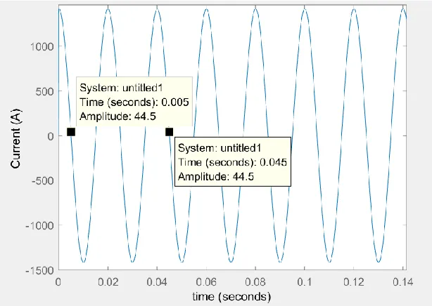
block in this model. Two periods in the graph are between 45ms and 5ms which is 40ms,
therefore, the frequency of the current is 2/40ms=50Hz, which is the system’s frequency
[image:38.612.161.468.163.381.2]as expected.
Figure 3.2 Current Inversion from DC (after boost converter) to AC with 50Hz (system frequency).
The third stage is to convert this current to instantaneous power because the output
of the conventional power system is power, thus, the input from the PV system to the grid
should also be in terms of power. The transfer function of this block can be obtained similar
to the method of obtaining 𝐺2. First, the instantaneous power p(t) is given by
𝑝(𝑡) =𝑉𝑚 𝐼𝑚
𝑖𝐴𝐶2 =
𝑉𝑚 𝐼𝑚
(𝐼𝑚cos (𝑤𝑡))2 =
𝑉𝑚𝐼𝑚 2 +
𝑉𝑚𝐼𝑚 (cos(2𝑤𝑡)) 2
The gain 𝑉𝑚
𝐼𝑚 is an impedance which is real without an imaginary part because the load is
purely resistive. Taking the Laplace transform of (3.6) gives,
𝑃(𝑠) =𝑉𝑚𝐼𝑚 2𝑠 +
𝑉𝑚𝐼𝑚 2
𝑠 𝑠2 + (2𝑤)2
where 𝑖𝐴𝐶 is the same expression obtained previously. Therefore, the transfer function for
the conversion from AC current to instantaneous power is:
(3.6)
22 𝐺3(𝑠) =
𝑃(𝑠) 𝑖𝐴𝐶(𝑠)
= (𝑉𝑚𝐼𝑚 2𝑠 +
𝑉𝑚𝐼𝑚 2
𝑠
𝑠2+ (2𝑤)2) ÷ (𝐼𝑚cos (𝑤𝑡))
= 𝑉𝑚((𝑠
2+ 𝑤2)(𝑠2+ (2𝑤)2)
𝑠2(𝑠2+ (4𝑤)2)
= 6351𝑠
4+ (1.88 × 10⁹)𝑠2+ (1.237 × 10¹⁴)
𝑠4+ (3.948 × 10⁵)𝑠2
It is noticed that the instantaneous power has double the frequency of the inverted
current because the equation of instantaneous power is given by the multiplication of two
cosine waves (the current and the voltage) each of which has a frequency of 50Hz, and by
the trigonometric identities which produces a cosine wave of double the frequency. Thus,
a frequency of 100Hz can be observed from Figure 3.3 for the instantaneous power. One
period occurs between 2.6ms and 12.6ms, i.e. 10ms giving a frequency of 1/10ms=100Hz.
The voltage and the current are in phase, therefore there is no reactive power going from
the PV array to the grid [14].
Figure 3.3 Instantaneous power from the photovoltaic system (100 Hz).
Since the load in the photovoltaic systems is purely resistive, the instantaneous
23
which is the case in Figure 3.3. This explains why the instantaneous power has double the
amplitude (9MW instead of 4.5MW), because the real negative peak of the original sine
wave is at -4.5MW, but with the offset that occurred, the negative amplitude shifted to the
positive side making the -4.5 start from 0 and the 4.5 peak to shift to 9MW.
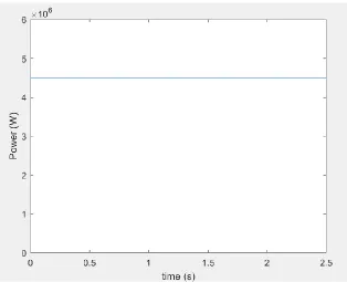
However, the required output power of the PV system that will be an input to the
conventional power system is the average power not the instantaneous in order to make
them compatible with each other [14]. Thus, the last stage here is to convert the
instantaneous power to average power. The equation for the average power in the time
domain is given by
𝑃𝑎𝑣𝑔 =
1
𝑇∫ 𝑣𝐴𝐶× 𝑖𝐴𝐶 𝑑𝑡
𝑇
0
= 1
𝑇∫ 𝑉𝑚cos(𝑤𝑡) . 𝐼𝑚cos(𝑤𝑡) 𝑑𝑡
𝑇
0
= 1 𝑇∫
𝑉𝑚𝐼𝑚 2 +
𝑉𝑚𝐼𝑚 (cos(2𝑤𝑡)) 2 𝑑𝑡 =
𝑇
0
𝑉𝑚𝐼𝑚 2
This is expected since the load is purely resistive, and the average power would be a
constant. The Laplace transform of the average power (𝑃𝑎𝑣𝑔) is given by
𝑉𝑚𝐼𝑚
2𝑠
To obtain the transfer function of the conversion from instantaneous power to average
power after simplification is given next as,
𝐺4(𝑠) = 𝑃𝑎𝑣𝑔(𝑠) 𝑝(𝑠) =
𝑉𝑚𝐼𝑚 2𝑠 ÷ (
𝑉𝑚𝐼𝑚 2𝑠 +
𝑉𝑚𝐼𝑚 2
𝑠
𝑠2+ (2𝑤)2) =
𝑠2+ (4𝑤)2
2(𝑠2+ (2𝑤)2)
= 𝑠
2+ (3.948 × 10⁵)
2𝑠2+ (3.948 × 10⁵)
Figure 3.4 shows the final output of the PV system which is the MPP average power
(4.5 MW) as expected because this is half of the amplitude of the offset instantaneous
power graph. If the power was not purely resistive, then the real power will be less than (3.9)
(3.10)
24
4.5MW because part of the graph of the instantaneous power will be below the x axis
depicting reactive power.
Figure 3.4 Average power output of the PV (second input to conventional power system).
Putting all the above blocks together leads to the full PV system which is shown in Figure
[image:41.612.148.462.119.374.2]3.5.
Figure 3.5 PV system designed model.
To get the state space model of this PV system, the form chosen here is the
controllable canonical one. This would lead to the state space model of the system in the
25
𝑥̇(𝑡) = 𝐴𝑥(𝑡) + 𝐵𝑢(𝑡)
𝑦(𝑡) = 𝐶𝑥(𝑡) + 𝐷𝑢(𝑡)
Starting with the DC-AC inverter block:
𝐺2(𝑠) =𝑖𝐴𝐶(𝑠) 𝐼2(𝑠) =
𝑠2 𝑠2+ 98700
The controllable canonical form is obtained from the following state equations,
𝑥7̇ = 𝑥8
𝑥8̇ = −98700𝑥7+ ∆𝑃𝑖
𝑦 = −98700𝑥7+ ∆𝑃𝑖
∆𝑃𝑖 in the following equations represent the input to each sub-system, giving the following
state space model,
[𝑥7̇ 𝑥8̇ ] = [
0 1 −98700 0] [
𝑥7
𝑥8] + [01] ∆𝑃𝑖
𝑦 = [−98700 0] [𝑥𝑥7
8] + [1]∆𝑃𝑖
Realizing this state space model as a block diagram is shown in Figure 3.6 below.
Figure 3.6 DC-AC inverter block to obtain controllable canonical form.
As to 𝐺3(𝑠), the same steps are applied to obtain the state space equations as follows:
𝑥3̇ = 𝑥4
26 𝑥4̇ = 𝑥5
𝑥5̇ = 𝑥6
𝑥6̇ = −3.948 × 10⁵𝑥5+ ∆𝑃𝑖
𝑦 = 1.237 × 10¹⁴𝑥3− 6.27375 × 10⁸𝑥5+ 6351∆𝑃𝑖
This leads to the state space model
[ 𝑥3̇ 𝑥4 𝑥5̇
𝑥6̇
̇
] = [
0 1 0 0
0 0 1 0
0 0 0 1
0 0 −3.948 × 10⁵ 0
] [ 𝑥3 𝑥4 𝑥5 𝑥6 ] + [ 0 0 0 1
] ∆𝑃𝑖
𝑦 = [1.237 × 10¹⁴ 0 −6.27375 × 10⁸ 0] [
𝑥3 𝑥4 𝑥5 𝑥6
] + [6351]∆𝑃𝑖
Figure 3.7 shows the detailed block diagram in canonical form for 𝑮𝟑.
Figure 3.7 Instantaneous power blocks to obtain controllable canonical form.
Similarly, 𝐺4(𝑠) state space model is given as follows:
𝑥1̇ = 𝑥2
𝑥2̇ = −197400𝑥1+ ∆𝑃𝑖
27 𝑦 = 197400𝑥1+1
2∆𝑃𝑖
In matrix form, we have
[𝑥1̇ 𝑥2̇ ] = [
0 1
−197400 0] [ 𝑥1
𝑥2] + [01] ∆𝑃𝑖
𝑦 = [197400 0] [𝑥𝑥1
2] + [1/2]∆𝑃𝑖
Figure 3.8 shows the corresponding block diagram in canonical form.
Figure 3.8 Average power block to obtain controllable canonical form.
Combining all these state space models for the sub-blocks into one state space
model gives the overall state space matrix (3.31). 𝐺2 is circled in red, 𝐺3 is circled in blue,
and 𝐺4 is circled in yellow.
A=
[
0 1 0 0 0 0 0 0
−197400 0 6.185 × 10¹³ 0 3.1368 × 10⁸ 0 3.13422 × 10⁸ 0
0 0 0 1 0 0 0 0
0 0 0 0 1 0 0 0
0 0 0 0 0 1 0 0
0 0 0 0 −3.948 × 10⁵ 0 −98700 0
0 0 0 0 0 0 0 1
0 0 0 0 0 0 −98700 0]
(3.28)
(3.29)
(3.30)
28 B= [ 0 6048 0 0 0 1 1.5× 2 0.7 0 1 1.5× 2 0.7]
C=[0 1 0 0 0 0 0 0]
D=[6048.57]
Notice that these sub-blocks are interconnected, therefore, these extra connections
need to be accounted for. The values written in green in the state matrix show the values
that accounted for the connection between the blocks.
To get these values of the interconnection, some state equations needed to be
modified. The modified state Equations 3.36 and 3.37 demonstrate how these values were
obtained. The term ∆𝑃𝑖 here in the full state matrix represents the input of the photovoltaic
system rather than the input of each sub-block separately.
𝑥2̇ = −197400𝑥1+
1
2[6351 (−98700𝑥7 + ( 1 1.5×
2
0.7) ∆𝑃𝑖] − ( 1
2× 6.2737 × 10
8𝑥 5)
+ (1
2× 1.237 × 10
14𝑥 3)
Simplifying Equation 3.35 gives:
𝑥2̇ = −197400𝑥1+6.185 × 10¹³𝑥
3−3.1368 × 10⁸𝑥5+3.13422 × 10⁸𝑥7
+ 6048.57∆𝑃𝑖
𝑥6̇ = −3.948 × 10⁵𝑥5− 98700𝑥7+ ( 1
1.5× 2 0.7) ∆𝑃𝑖
In addition, to get the D matrix, the following calculation has been done by tracking
how the output is directly related to the input. Or, it can also be obtained directly from the
final 𝑥2̇ equation.
29 1
2× 6351 × 2 0.7×
1
1.5= 6048.57
The full system in the form that allows us to deduce the state space matrix and cast
it in the controllable canonical form is given in Figure 3.9. An additional model that was
also useful in some calculations is the full transfer function of the PV system shown in
Equation 3.39, where ∆𝑃𝑖 = 𝑃𝑉𝑎𝑟𝑟𝑎𝑦; or the output of the PV array which is the input to
the PV system.
𝑃𝑎𝑣𝑔 𝑃𝑉𝑎𝑟𝑟𝑎𝑦 =
8402 𝑠8+ (5.805𝑒09) 𝑠6+ (1.146𝑒15) 𝑠4 + (6.462𝑒19) 𝑠2
1.4 𝑠8+ (9.672𝑒05) 𝑠6+ (1.909𝑒11) 𝑠4+ (1.077𝑒16) 𝑠2
(3.38)
31
3.2
Thermal Power System – Single Area
The state space model of the single-area power system (thermal) with only the
integral controller is presented in this section. Table 3.1 shows the parameters that were
used in the modeling of the thermal power system under study and their definition.
Table 3.1 Parameters of the thermal power system.
Parameter Definition Value
𝑻𝒈 Governor time constant 0.08
𝑹 Droop 2.4
𝑻𝒕 Turbine time constant 0.3
𝑻𝒓 Reheater time constant 10
𝑲𝒓 Reheater gain 0.5
𝑻𝒑 Generator time constant 20
𝑲𝒑 Gain constant 120
Figure 3.10 shows this part of the system without any controller. The first input to
this system is the speed changer ∆𝑃 that determines the amount of fuel coming in to the
system by operating the valve. The state space model (in Equations 3.40 and 3.41) with
∆𝑃𝑙𝑜𝑎𝑑 being the second input which represents the changes in the power system load
(disturbance).
32 [
𝑥1̇
𝑥2̇ 𝑥3̇
𝑥4̇
] =
[ −1
20 6 0 0
0 −0.1 −1.566 5 3
0 0 −1
0.3
−1 0.3 −5.21 0 0 −12.5]
[ 𝑥1 𝑥2 𝑥3 𝑥4 ] + [ −6 0 0 0
] ∆𝑃𝑙𝑜𝑎𝑑
𝑦 = [1 0 0 0] [ 𝑥1
𝑥2
𝑥3
𝑥4
]
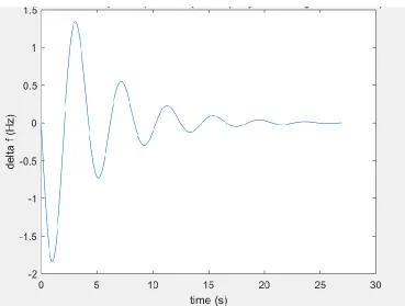
The frequency error response of this system due to a sudden 50% increase in the
load is given in Figure 3.11 with the corresponding response specifications in Table 3.2.
SSE represents the steady state error.
Table 3.2 Response summary due to a 50% increase in load.
Settling Time (s) 18.2
Undershoot (Hz) -2.33299
SSE (Hz) -1.175
Figure 3.11 Response of the single-area thermal power system due to a 50% increase in load without any controller.
(3.40)
33
Since one of the main criteria to be met in the system is a zero steady state frequency
error, the addition of an integral controller is needed for this purpose. In this section, the
integral controller is integrated in the state space model since it will introduce an additional
state variable in the original state space model. Thus, to apply the other controllers later, it
is important to work with this updated state space model so that the final steady state error
criteria is ensured to be met. Therefore, from this point onwards in this work, the model
will always have an integral controller integrated. This way SSE will always be 0, and only
the settling time and undershoot are to be considered. Adding an integral controller to the
system increases the number of state variables by 1, thus, the system now has a total of 5
state variables. Figure 3.12 shows the thermal power system with the integral controller.
Figure 3.12 Block diagram of the single-area thermal power system with integral controller only.
After adding the integral controller and tuning its gain value to the one that
produced the best response (𝑘𝑖 = 0.6), the new state equations become,
𝑥1̇ = 1
20𝑥1 + 6𝑥2− 6∆𝑃𝑙𝑜𝑎𝑑
𝑥3̇ = 1 0.3𝑥3−
1 0.3𝑥4
Substituting this expression of 𝑥3̇ into the equation of 𝑥2̇ gives
𝑥2̇ = −0.1𝑥2− 1.566𝑥3+
5 3𝑥4
(3.42)
(3.42)
34
The remaining two state equations to complete the 5 are:
𝑥4̇ −= 1
2.4 × 0.08𝑥1− 1 0.08𝑥4−
1 0.08𝑥5
𝑥5̇ = 𝑘𝑖× 𝑥1
Accordingly, the state space model of the thermal power system with an integral
controller is given in (3.46) and (3.47). The first input to the thermal power system is
replaced by the effect of adding the integral controller, thus, only ∆𝑃𝑙𝑜𝑎𝑑 remains as the
input here.
[ 𝑥1̇
𝑥2̇ 𝑥3̇ 𝑥4̇
𝑥5̇ ] =
[ −1
20 6 0 0 0
0 −0.1 −1.566 5
3 0
0 0 −1
0.3
1
0.3 0 −5.21 0 0 −12.5 −12.5
𝑘𝑖 0 0 0 0 ]
[ 𝑥1
𝑥2
𝑥3
𝑥4
𝑥5]
+ [ −6 0 0 0 0 ] ∆𝑃𝑙𝑜𝑎𝑑
𝑦 = [1 0 0 0 0]
[ 𝑥1 𝑥2 𝑥3 𝑥4 𝑥5]
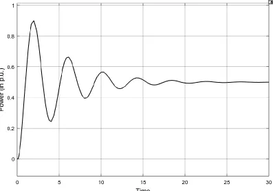
Figure 3.13 shows the frequency error response of this updated state space model.
Table 3.3 summarizes the key response specification values from the response.
(3.44)
(3.45)
(3.46)
35
[image:52.612.117.486.71.350.2]Figure 3.13 Single-area thermal power system frequency error response to a 50% increase in load (with integral controller only).
Table 3.3 Response summary of the single-area thermal power system for a 50% increase in load.
Settling Time (s) 19.716575
Undershoot (Hz) -1.8399269
SSE (Hz) 0
The controllability and observability of the system are checked to ensure that the
system can be controlled. Both the controllability matrix and observability matrix have a
rank of 5 which is equal to the number of state variables. Therefore, the system is
controllable and observable, and controllers can be designed and applied to the system.
In addition, to check the stability of the open loop system, the eigenvalues were
verified, and they are: -12.875, -2.475, -0.1995, -0.2168 + 1.525i and -0.2168 -1.
![Figure 1.1 a PV system connected to the load in the grid directly [6].](https://thumb-us.123doks.com/thumbv2/123dok_us/31813.2527/19.612.113.486.98.367/figure-pv-connected-load-grid-directly.webp)