eQuIPS: eQTL Analysis Using Informed Partitioning of SNPs – A Fully Bayesian Approach

This is a repository copy of

eQuIPS: eQTL Analysis Using Informed Partitioning of SNPs –

A Fully Bayesian Approach

.

White Rose Research Online URL for this paper:

http://eprints.whiterose.ac.uk/95043/

Version: Accepted Version

Article:

Boggis, E.M., Milo, M. and Walters, K. (2016) eQuIPS: eQTL Analysis Using Informed

Partitioning of SNPs – A Fully Bayesian Approach. Genetic Epidemiology, 40 (4). pp.

273-283. ISSN 1098-2272

https://doi.org/10.1002/gepi.21961

This is the peer reviewed version of the following article: Boggis, E. M., Milo, M. and

Walters, K. (2016), eQuIPS: eQTL Analysis Using Informed Partitioning of SNPs – A Fully

Bayesian Approach. Genet. Epidemiol., 40: 273–283, which has been published in final

form at http://dx.doi.org/10.1002/gepi.21961. This article may be used for non-commercial

purposes in accordance with Wiley Terms and Conditions for Self-Archiving

(http://olabout.wiley.com/WileyCDA/Section/id-828039.html)

[email protected] https://eprints.whiterose.ac.uk/ Reuse

Unless indicated otherwise, fulltext items are protected by copyright with all rights reserved. The copyright exception in section 29 of the Copyright, Designs and Patents Act 1988 allows the making of a single copy solely for the purpose of non-commercial research or private study within the limits of fair dealing. The publisher or other rights-holder may allow further reproduction and re-use of this version - refer to the White Rose Research Online record for this item. Where records identify the publisher as the copyright holder, users can verify any specific terms of use on the publisher’s website.

Takedown

If you consider content in White Rose Research Online to be in breach of UK law, please notify us by

eQuIPS: eQTL analysis using informed partitioning of SNPs - a

fully Bayesian approach

E. M. Boggis1, M. Milo2, K. Walters1,∗

1 School of Mathematics and Statistics, University of Sheffield, Sheffield, UK 2 Department of Biomedical Science, University of Sheffield, Sheffield, UK

∗ E-mail: [email protected]

Abstract

We develop a Bayesian multi-SNP MCMC approach that allows published functional significance

scores to objectively inform SNP prior effect sizes in eQTL studies. We developed the Normal

Gamma prior to allow the inclusion of functional information. We partition SNPs into pre-defined

functional groups and select prior distributions that fit the group-specific observed functional

sig-nificance scores. We test our method on two simulated datasets and previously analysed human

eQTL data containing validated causal SNPs. In our simulations the modified Normal Gamma

always performs at least as well, and generally outperforms, the other methods considered. When

analysing the human eQTL data we placed all SNPs into their actual functional group. The ranks

of the four validated causal SNPs analysed using the modified Normal Gamma increase

dramati-cally compared to those of the other methods considered. Using our new method, three of the four

validated SNPs are ranked in the top 1% of SNPs and the other is in the top 2%. For the standard

Normal Gamma, the best of the other methods, the four validated SNPs had ranks in the top 1%,

4%, 20% and 59%. Crucially these substantive improvements in the ranks make it highly likely

that most, if not all, of these validated SNPs would have been flagged for follow-up using our new

method whereas at least two of them would certainly not have been using the current approaches.

Introduction

Expression quantitative trait locus (eQTL) studies have successfully identified both cis-acting loci

(those that have an effect in the vicinity of their location) and trans-acting loci (those that act

at a distance). With the fall in the cost of sequencing and gene expression quantification they

challenges is that they tend to have a small number of individuals (small n) but a large number

of SNPs (large p). This means that eQTL studies, as with genome-wide association studies, are

both computationally intensive and, because the vast majority of SNPs are not expected to affect

gene expression, require the use of non-standard statistical techniques that implicitly model this

sparsity.

Many different multivariate statistical methods have been applied to this problem. The

statis-tical approaches we consider to model eQTL data without functional information can be divided

into two categories: fully Bayesian approaches via Markov Chain Monte Carlo (MCMC) and

meth-ods that use a maximum a posteriori (MAP) estimation approach that reports only the posterior

mode. Within the fully Bayesian approach, there are two categories of priors: variable selection

priors which use priors with point masses at 0; and continuous shrinkage priors with a lot of mass

near to 0. The latter shrink many parameter estimates close to, but not equal to zero. Bayesian

continuous shrinkage prior distributions tend to have a sharp mode at 0, with the mass in the tails

influencing the amount of shrinkage applied to large estimates.

We assess three fully Bayesian approaches: piMASS [Guan and Stephens, 2011], Spike and slab

(SS) [Ishwaran and Rao, 2005] and the Normal Gamma (NG) [Griffin and Brown, 2010] (of which

the Bayesian Lasso [Park and Casella, 2008] is a special case). piMASS and SS both use variable

selection through indicator variables to select explanatory variables to include in the model giving

truly sparse models. Using proximity of the SNPs and their marginal associations with respect to

gene expression, piMASS selects a different SNP set in every iteration. SS uses no such criteria for

SNP inclusion. The NG updates estimates for all SNPS at every iteration. piMASS, SS and the NG

share many similarities in the prior hierarchies, with the fundamental difference being the inclusion

or omission of a point mass at zero. As well as fully Bayesian methods, we also consider HyperLasso

(HL), a penalized regression approach equivalent to MAP estimation with a specific prior which

has the LASSO as a special case. The HL has a flexible two-parameter normal exponential gamma

prior whereas the LASSO has a single parameter constrained Laplacian (double exponential) prior.

Consequently we use HL to represent the Bayesian MAP estimation techniques. We also evaluate

the performance of least squares (LS) if n≥p or minimum length least squares (MLLS) if n < p

in order to compare with a univariate frequentist approach.

to good effect in eQTL studies. We create a framework that enables us to include SNP-specific

functional information and can be used to prioritise SNPs for follow up. Other approaches to

including functional information have been developed. Lirnet [Lee et al., 2009] for example allows

the incorporation of functional information, but not on a SNP-specific level. All of the previously

mentioned, multivariate statistical methods that do not currently allow the incorporation of

SNP-specific functional information could be modified to do so.

Based on its superior performance we developed the NG to include functional information. We

choose to use the Functional Significance (FS) Score [Lee and Shatkay, 2009] which is a normalized

score (FS ∈[0,1]) which combines information on the deleterious effects of SNPs from 16 publicly

available web services and databases. We used the FS scores for 112,949 SNPs, of which 1,399 are

known to be disease related, provided by the authors.

In this paper we compare the performance of eQTL detection using the NG, SS, HL and piMASS

and standard least squares (LS) or minimum length least squares (MLLS). Performance is assessed

by comparing the ranks of relevant posterior estimates of simulated causal SNPs through receiver

operator characteristic (ROC) curves. We test our development of the NG on two simulated data

sets and data from the Fairfax eQTL study [Fairfax et al., 2012] which measured gene expression in

primary monocytes and B cells. The Fairfax data contains validated causal SNPs and we compare

the rank of these validated causal SNP in the NG and our NG developed to include functional

information.

Methods

In this section we briefly describe the methods we compare.

Least Squares (LS)

The standard vector form of a linear model isY =α+βX+ǫwhereXis an n×p matrix of SNP

genotypes,Y is a vector of gene expression values,βis a vector of effect sizes andǫ∼Np(0, σ2In).

The standard LS estimates are given byβb= (XT_X)−1_XT_{Y ifp < n. Ifp > n, as for most eQTL}

data, we use the minimum length least squares (MLLS) estimates given by ˆβ = (XT_X)†_XT_Y

Spike and Slab (SS)

The SS (a form of Bayesian Variable Selection Regression) was initially proposed by Mitchell and

Beauchamp [1988] and involves a mixture prior distribution consisting of the Normal distribution

and point mass at 0. Let p be the number of SNPs and n be the number of observations, y be

an n-vector of gene expression values, γ = diag(γ1, . . . , γp) be the binary vector indicating which

SNPs are in the model, βγ be the effect size parameter vector for those SNPs in the model, Xγ

be the genotype design matrix for those SNPs in the model, πk be the prior inclusion probability

of SNP k, V_γ−1 be the rows and columns of V−1 = (XT_{X + diag(X}T_{X))/2n corresponding to}

γk = 1 and σ2 be the error variance. Then the standard hierarchical set-up for SS can be seen in

Equations (1) - (5).

γ ∼

p

Y

i=1

πiγi(1−πi)1−γi (1)

σ2 ∼ Ga(0.001,0.001) (2)

σ−_ǫ2 ∼ Ga(0.005, κ/2) (3)

βγ|γ, σ

2

ǫ ∼ N(0, σǫ2(Vγ−1)−1) (4)

y|βγ,Xγ, σ2 ∼ Nn(Xγβγ, σ2In). (5)

where κ is taken to be 0.005s2

y and s2y is the marginal standard deviation of the response. SS

reports the posterior probability of inclusion (having a non-zero regression coefficient) as its measure

of association as well as estimating the posterior regression effect sizes conditional on being in the

model.

For our simulation results, we use a prior inclusion probability of 0.05 for all SNPs unless

otherwise stated. There are two possible post burn-in posterior estimators for βk for the SS: the

posterior mean of βk and the proportion of MCMC iterations with βk 6= 0. The posterior mean

gave the largest AUC from a ROC analysis so we used this as the summary statistic for the SS.

piMASS

piMASS [Guan and Stephens, 2011] is another form of Bayesian Variable Selection Regression with

case-control) studies. It makes proposals of which SNPs to include at the next iteration based on the

genetic distance between, and marginal associations of, the SNPs not currently in the model. We

compared two posterior estimators from piMASS: the posterior mean ofβj and the the proportion

of MCMC iterations with βj 6= 0. The posterior mean of βj performed best in terms of the AUC

from a ROC analysis so we used this to assess the performance of piMASS. We used the default

values of the hyperparameters.

HyperLasso (HL)

HL [Hoggart et al., 2008] is a Bayesian-inspired approach that determines Maximum-a-Posteriori

(MAP) estimates of the parameters rather than sampling from the posterior distribution. The

normal exponential gamma prior of HL is a continuous distribution with a sharp mode at zero and

can have heavy tails for certain combinations of the shape and scale hyperparameters. The large

mass around zero in conjunction with the heavy tails of the prior forces parameters with maximum

likelihood estimates close to zero to be shrunk to zero with reduced shrinkage on those variables

with larger maximum likelihood estimates.

The posterior of the HL is not always unimodal, especially in the n < p case, and the order

in which the coefficients are updated also affects the MAP estimate, particularly in the case of

highly correlated SNPs. The software tries to overcome this by implementing multiple runs of the

algorithm. One of the drawbacks to HL is the high sensitivity of the posterior estimates to the

choice of hyperparamters. The authors provide some guidance about appropriate hyperparameter

values in the case-control study setting, based on controlling the family-wise error rate, but don’t

for eQTL studies. We experimented with different values of the scale parameter from 100 to 0.001

but found that the AUC was maximized using the default value of 0.1.

The Normal Gamma prior (NG)

As for HL, the NG prior belongs to the family of scale mixtures of normals. The NG is a

2-parameter generalisation of the single-2-parameter double exponential prior (see equation (8) in

which the idiosyncratic variance of the conditional distribution of βi has a 2-parameter gamma

distribution). The key feature of the 2-parameter NG is that the prior structure allows adaptive

and Brown [2010] propose a hierarchical structure for each effect size parameter βi defined in

Equations (6)-(9), with uninformative priors onα and σ2.

π(λ)∼Ex ₁

2

(6)

π(γ−2|λ)∼Ga

2,M

2λ

(7)

π(ψi|λ, γ−2)∼Ga

λ, 1

2γ2

(8)

π(βi|ψi)∼N(0, ψi). (9)

M is the expectation of the prior marginal variance ofβi which is estimated as the mean square

of the maximum likelihood estimates of the βi parameters. The marginal prior variance of the

effect sizes is var (π(βi|λ, γ)) = 2λγ2. As is standard in Bayesian analysis this variance is given an

inverse gamma distribution IG(2,M) having expectation M. This yields the gamma conditional

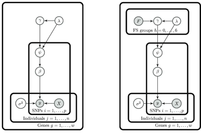
distributionγ−2|λ. given in equation (7). The left hand side of Figure 1 shows the directed acyclic

graph (DAG) for this model. The parameters are updated via MCMC using a Metropolis-Hastings

within Gibbs approach. We compared several posterior summary statistics for the NG: the mean,

median, interquartile range and whether the credible interval contained 0. The summary statistic

giving the greatest AUC was the posterior mean so we used this as our summary statistic for the

NG. The full conditionals used in the MCMC updating for the NG are given in Supplementary

Text S1.

Details of the MCMC set up

The NG and SS are run for 100,000 iterations for the simulated and Fairfax data with a 5,000

iteration burn-in. piMASS is run for 100,000 iterations with a 10,000 iteration burn-in and thinning

based on maintaining every 10th iteration, as suggested in the documentation.

Details of the simulated eQTL datasets

We used HapGen2 [Su et al., 2011] to simulate data based on the known SNP correlation structure

in the human genome. HapGen2 generates DNA sequences based on the minor allele frequency

samples of the European haplotypes of the August 2010 release of the 1000 genomes data [Altshuler

et al., 2010] for our simulations.

We simulated data with a sample size of 300 for 631 SNPs from the region around the

CAS-PASE8 gene on chromosome 2 - a region widely believed to be associated to breast cancer and

melanoma [Barrett et al., 2011, Camp et al., 2012]. A 200kbase region (from 201566128 to 201766128

in the human genome 19 build of chromosome 2) surrounding the CASPASE8 gene was used for

simulations. This region has a variety of LD block sizes and strengths allowing us to evaluate the

effectiveness of the NG in detecting causal SNPs from a wide range of underlying LD structures.

We simulated 6 causal SNPs which is more than would typically be expected in a region of

this size but we wanted to place the causal SNPs in a variety of LD block sizes and strengths.

Three causal SNPs were chosen to be in high LD with each other, 2 were chosen to be in moderate

LD with each other and 1 was chosen to be in very low LD with all the other causal SNPs. Two

datasets were simulated - one with all causal SNPs having a MAF of approximately 0.2 (data set

2A) and the other with a MAF of approximately 0.02 (data set 2B). The causal SNPs are different

in the 2 datasets to ensure the SNPs have the required MAF.

We simulated the ith _{gene expression (y}

i) as yi = Ppj=1xijβj +ǫi where ǫi ∼ N(0,1), xij

represents thejth _{genotype for personi, andβ}

j represents the effect size of thejth SNP. All effect

sizes were simulated to be 0.4. For simplicity, when simulating the gene expression value, we use

the dominant modelling of SNPs, where 0 represents the homozygous wild-type genotype and 1

represents all other genotypes. The error included in the gene expression value is used to represent

the noise seen in experimental data. The effect sizes and number of SNPs in the region were chosen

to be consistent with other simulated datasets [Kang et al., 2012, Petersen et al., 2013, Wu et al.,

2011].

Details of the Fairfax dataset

The Fairfax study [Fairfax et al., 2012] was designed to look for cis- and trans-acting eQTLs

in paired purified primary monocytes and B-cells. The study aimed to identify effects unique to

monocytes or B-cells via cell-specific eQTLs. The data was obtained using Illumina Human HT-12

v4 BeadChip for the genome-wide expression profiling and Illumina HumanOmniExpress-12v1.0

We analysed four of the probe sets reported in Figure 6b of Fairfax et al. [2012] to assess our

statistical methods. To reduce the number of SNPs we kept all exonic SNPs on the chromosome

where the gene of interest was located and any SNPs that were reported as causal regardless of the

location (exonic, intronic, or otherwise). Table 1 gives details of the final numbers of SNPs and

individuals for each of the 4 probe sets considered. In each gene there is a single validated causal

SNP. We used Impute2 [Howie et al., 2009] to estimate the missing genotypes. We retained only

those imputed genotypes for which the info score was greater than 0.3. We removed individuals

with a high proportion of imputed SNPs with low information scores.

The results in Figure 6b of Fairfax et al. [2012] show that the number of copies of the rare allele

has a clear effect on gene expression, therefore we recoded the SNPs as 0,1,2 to reflect the additive

effect of the number of copies of the minor allele. Histograms of the gene expression values for the

four genes in Table 1 are provided in Supplementary Text S2.

Gene name n p Causal SNP (MAF)

CARD9 mono 243 511 rs4266763 (0.350)

RBM6 mono 243 932 rs1061474 (0.325)

RBM6 bcell 243 932 rs1061474 (0.325)

FADS1 bcell 243 1076 rs174548 (0.486)

Table 1: The gene names, number of individuals (n), number of SNPs (p), causal SNP rs number and its minor allele frequency (MAF) for the four genes selected from Fairfax et al. [2012].

Including the FS score into the NG framework

The NG showed the best performance in ranking SNPs in our simulated data so we developed

the NG to include relevant functional information. We call this modification the Normal Gamma

Splitting Function (NGSF). Functional information has started to be included in population-based

association studies with some success [Pickrell, 2014, Spencer et al., in press]. In each analysis

where we include functional information we partition our SNPs into a maximum of 7 functional

groups (intergenic, splicing etc). For each group we select all SNPs of the same type from the

online FS score resource and fit densities to the empirical distribution of the FS scores. We choose

to include the functional information in the NG via the expectation of the marginal prior variance

of β. This allows the functional significance score to inform, a priori, the effect sizes of all SNPs

Figure 1: Directed acyclic graphs (DAGs) for the standard Normal Gamma (left) and the Normal Gamma including functional information from the FS scores (right). The DAGs highlight the observed variables (grey) and parameters (white) that relate to SNPs, individuals, FS score groups or genes.

the inverse gamma density. When we include functional information, M is replaced with B so

that var (π(βi|λ, γ)) = 2λγ2 ∼IG(2,B), where B is a monotonic transformation of the observed

functional informationF. We useB rather thanF directly becauseF ∈[0,1] which we found to be

too narrow for our purposes. We letB = tan

F πǫ

2

+ (1−ǫ) withǫ= 0.99 so thatB ∈[0.01,63.7]

which we found to be sufficiently wide to facilitate differential shrinkage in the different SNP groups.

The directed acyclic graph on the right of Figure 1 shows how the FS score,F, is included in the

NG framework.

Prior distributions for F

We fitted empirical prior distributions to the raw FS score values for each SNP type which makes

the computation of the full conditionals more computationally expensive but ensures that we are

using truly representative distributions for these groups. The fitted densities are shown in Figure 2

and the distributions are given in Equations (10)-(16).

We chose the Bernoulli probability distribution for SNPs in splicing regions because we

consid-ered them to either have a highly deleterious effect or to have no effect at all. We choose a Bernoulli

Intergenic FS score

Density

0.0 0.2 0.4 0.6 0.8 1.0

0

10

Intronic FS score

Density

0.0 0.2 0.4 0.6 0.8 1.0

0

3

6

UTR3 FS score

Density

0.0 0.2 0.4 0.6 0.8 1.0

0

2

4

Splicing FS score

Density

0.0 0.2 0.4 0.6 0.8 1.0

0

3

Other FS score

Density

0.0 0.2 0.4 0.6 0.8 1.0

0

3

6

Synonymous FS score

Density

0.0 0.2 0.4 0.6 0.8 1.0

0.0

2.0

Non−synonymous FS score

Density

0.0 0.2 0.4 0.6 0.8 1.0

0.0

1.5

gives a Bernoulli(₁₀₅53) prior distribution for splicing SNPs. Most other distributions are mixtures

of gamma distributions and point masses, not always at zero.

π(FIntergenic)∝1F∈[0,1]

0.789δ[0.101866]+ 0.211Ga(1.296,6.365) (10)

π(FIntronic)∝1F∈[0,1]

0.121δ_[0]+ 0.879Ga

7.359, 1

0.0235

(11)

π(FUTR3)∝1F∈[0,1]{Ga(1.45,8.08)} (12)

π(FSplicing)∼Bernoulli

53 105

(13)

π(FOther)∝1F∈[0,1]

0.085δ_[0]+ 0.915Ga

4.349, 1

0.0340

(14)

π(FSyn)∝1F∈[0,1]

0.946Ga

2.929, 1

0.113

+ 0.054Ga

640.5, 1

0.0015

(15)

π(FNon-syn)∼Uniform[0,1]. (16)

where δ[a] represents a point mass at a and 1F∈[0,1] is an indicator function taking the value 1 if F ∈ [0,1], and 0 otherwise. The hyper-parameter values in equations (10) to (16) are derived

directly from the fitted densities in Figure 2. The full conditionals for the NGSF are given in the

Appendix.

Results

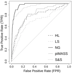
Comparing the performance of the selected methods on the simulated datasets

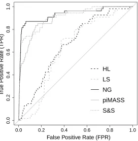
Figures 3 and 4 show the ROC curves comparing the performance of the methods on datasets 2A

(causal MAF 0.2) and 2B (causal MAF 0.02) respectively. Table 2 reports the area under the ROC

curves (AUC) for each method. The NG and SS have considerably higher AUCs when applied to

dataset 2A than LS, HL or piMASS. LS has an AUC of 0.6917 which is the worst of the methods

considered. For dataset 2B (MAF 0.02), Table 2 shows that piMASS performs better in terms of

AUC than in dataset 2A and has an AUC approaching that of the NG and SS. HL and LS again

have the lowest AUCs. For both datasets 2A and 2B the NG prior has the highest AUC followed

closely by SS. LS, HL and piMASS all run in less than an hour on a desktop pc with a 2 GHz

an average of 15 hours. SS took several hours on average but less than the NG.

Method

Dataset HL LS NG piMASS SS

2A 0.7809 0.6917 0.9702 0.8093 0.9418

2B 0.6667 0.6343 0.9322 0.8999 0.9119

Table 2: AUCs for the ROC curves for the 5 methods applied to simulated datasets 2A and 2B with a sample size of 300 and 631 SNPs. Each of the 9 simulated data sets has 6 causal SNPs each with simulated effect sizes of 0.4. The MAF of the causal SNPs in dataset 2A (2B) is approximately equal to 0.2 (0.02) and the data are simulated using the LD structure of the CASPASE8 region using HapGen2 [Su et al., 2011].

0.0

0.2

0.4

0.6

0.8

1.0

0.0 0.2 0.4 0.6 0.8 1.0

T

rue P

ositiv

e Rate (TPR)

False Positive Rate (FPR)

HL

LS

NG

piMASS

S&S

0.0

0.2

0.4

0.6

0.8

1.0

0.0 0.2 0.4 0.6 0.8 1.0

T

rue P

ositiv

e Rate (TPR)

False Positive Rate (FPR)

HL

LS

NG

piMASS

S&S

Figure 4: ROC curve comparing the 5 statistical methods applied to simulated dataset 2B with a sample size of 300 and 631 SNPs. Each of the 9 simulated data sets has 6 causal SNPs each with a MAF approximately equal to 0.02 and an effect size of 0.4. The data are simulated using the LD structure of the CASPASE8 region using HapGen2 [Su et al., 2011].

Including Functional Information

In this section we assess the effect of implementing the NGSF. The NGSF has a standard NG

hierarchical structure but uses functional information in the form of the FS score to enable

differ-ential shrinkage between the 7 SNP groups. Within the simulated data sets we allocated all 625

non-causal SNPs to SNP groups randomly whilst ensuring that the proportions in each SNP group

were approximately the same as those used to determine the priors shown in Figure 2. We then

consider two separate scenarios: in the first the 6 causal SNPs are placed in the UTR3 group (NG

UTR), in the second they are placed in the Splicing group (NG splicing). We choose these two

groups because they represent SNPs that are,a priori, unlikely to be deleterious and very likely to

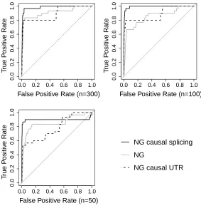
Comparing the ranking performance of the NGSF and NG on simulated data

We compare the ranks of the causal SNPs using the NGSF in our two scenarios with those from the

standard NG using ROC curves. Figure 5 shows ROC curves forn= 50,100 and 300 separately to

assess the effect of the sample size (n). The NG splicing detects the highest proportion of causal

SNPs at the lowest false positive rate (FPR) when the FPR is less than 0.5 which is the most

relevant part of the ROC space. These results show that the NGSF has the desirable property

that when the causal SNPs are together in a group that a priori has a high probability of being

deleterious, the posterior mean effect sizes are larger than when the causal SNPs are in a group

which isa priori less likely to be deleterious (and hencea priori has smaller effect sizes).

0.0

0.2

0.4

0.6

0.8

1.0

0.0 0.2 0.4 0.6 0.8 1.0

T

rue P

ositiv

e Rate

False Positive Rate (n=300)

0.0

0.2

0.4

0.6

0.8

1.0

0.0 0.2 0.4 0.6 0.8 1.0

T

rue P

ositiv

e Rate

False Positive Rate (n=100)

0.0

0.2

0.4

0.6

0.8

1.0

0.0 0.2 0.4 0.6 0.8 1.0

False Positive Rate (n=50)

T

rue P

ositiv

e Rate NG causal splicing

NG

NG causal UTR

Figure 5: ROCs showing the ranks of the posterior mean effect sizes for 6 causal SNPs in data set 2A for the NG, NG splicing and NG UTR scenarios forn= 300,n= 100 andn= 50. Five replicate data sets were simulated in HapGen2 [Su et al., 2011] using the LD structure of the CASPASE 8 region in which all the causal SNPs had a MAF of approximately 0.2 in the population. The NG splicing (NG UTR) case is where all 6 causal SNPs are defined as splicing (UTR3) and all 625 non-causal SNPs are from the other 6 functional information groups.

curve in Table 3. For each sample size considered, the NG splicing has the largest AUC. The

relative performance of the NG and the NG UTR is less clear. Forn= 100 the NG has the lowest

AUC, but forn= 50 andn= 300, the AUC of NG UTR is lowest although forn= 300 the NG and

NG UTR have very similar AUCs. Becausen < p in our eQTL data, it is important to determine

the sensitivity of the results to the sample size which affects the information in the likelihood.

By inspecting the columns of Table 3 we see the relative influences of the prior and likelihood in

determining the AUCs. For both the NG UTR and NG splicing, when n= 50 the prior strongly

influences the ranking and the posterior effect sizes of the causal SNPs are substantially shrunk

compared to those in the n= 100 case. There is very little difference between the performance of

either the NG UTR or the NG splicing at n= 300 compared ton= 100. The sample size affects

the performance of the NG differently. For the NG the prior enforces similar amounts of shrinkage

in then= 50 andn= 100 cases. It is not untiln= 300 that we start to see less shrinkage of causal

SNPs relative to the non-causal SNPs. Perhaps the most important observation is that even with

modest eQTL sample sizes as low as 100, placing the causal SNPs in the group with ana priori low

probability of a deleterious effect gives AUCs which are comparable to the standard NG. It appears

that just partitioning the SNPs and allowing differential shrinkage can substantially improve causal

eQTL rankings.

NG NG splicing NG UTR

n= 300 0.9103 0.9848 0.8945

n= 100 0.8544 0.9931 0.8873

n= 50 0.8526 0.8985 0.7825

Table 3: The AUC of the ROC curves in Figure 5

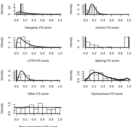
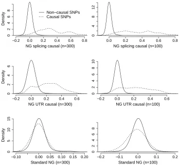
Comparing posterior mean effect sizes of the NGSF and NG on simulated data

Previous analyses have concentrated on the ranks of the causal SNPs. Next we focus on posterior

effect size estimation. Figure 6 shows kernel density estimates of the posterior mean effect sizes

for all causal and non-causal SNPs for NG splicing, NG UTR and the standard NG. The posterior

effect sizes for the causal SNPs in the NG splicing are larger than for NG UTR, especially for

n = 300, confirming the conclusions from our previous ROC analysis. The causal SNPs have

particular we notice that, even in the NG UTR case, where the prior puts a lot of mass at low FS

scores, there appears to be less shrinkage in the posterior mean effect size estimates compared to

the NG. The ROC analysis from the previous section gave similar AUCs for the NG and NG UTR

for n≥100. Here we see that although the ranks of the two approaches are similar (resulting in

similar AUCs), the posterior mean effect sizes of the causal SNPs for NG UTR are more clearly

separated from those of the non-causal SNPs than they are in the NG analysis. So allocating all

the causal SNPs to a single prior group results in superior detection of the causal SNPs, even if

causal SNPs are placed in groups with an a priori low probability of being deleterious.

−0.2 0.0 0.2 0.4 0.6 0.8

0

2

4

6

8

NG splicing causal (n=300)

Density

Non−causal SNPs Causal SNPs

0.0 0.2 0.4 0.6 0.8

0

4

8

12

NG splicing causal (n=100)

−0.2 0.0 0.2 0.4 0.6

0

2

4

6

NG UTR causal (n=300)

Density

−0.2 0.0 0.2 0.4 0.6

0

2

4

6

8

10

NG UTR causal (n=100)

−0.10 0.00 0.05 0.10 0.15 0.20

0

5

10

15

Standard NG (n=300)

Density

−0.2 −0.1 0.0 0.1 0.2

0

2

4

6

8

Standard NG (n=100)

Assessing the results of the NGSF with causal SNPs split across functional information groups.

There are only likely to be a small number of causal SNPs within a gene so it is reasonably likely

that they will all belong to one of the functional groups we have defined but we also assess the

effect of splitting the 6 causal SNPs across the UTR3 and Splicing functional groups by placing 3

in each group (labelled as NG mixed). The SNPs in the splicing group have an average posterior

mean rank of 3 whereas SNPs in the UTR3 group have an average posterior mean rank of 13.5.

Figure 7 shows the ROC curve for the NG mixed case in comparison to placing all the causal SNPs

in the same functional group. When the causal SNPs are split across groups, the AUC is 0.8564

which is somewhat smaller than the AUCs of the NG, NG UTR and NG splicing. Importantly

however, at relevant FPRs of less than 20%, the TPR of the NG mixed is consistently at or above

that of the NG and NG UTR.

Comparing the performance of the NG and NGSF on the Fairfax data

Our Fairfax data analysis includes SNPs in exonic regions on the same chromosome as the gene

under consideration in addition to all validated causal SNPs, not all of which were exonic. This

is true of the FADS1 bcell gene, where the validated causal SNP is intronic and is the only SNP

in its category. The causal SNPs are exonic in the CARD9 mono, RBM6 mono and RBM6 bcell

probe sets. There were some exonic SNPs with unknown synonymous /non-synonymous status. We

allocated these SNPs to the ‘other’ category (see Figure 2 for prior FS score plots). We performed

the analysis separately for each of the 4 probe sets. Table 4 shows the number of SNPs in each

group.

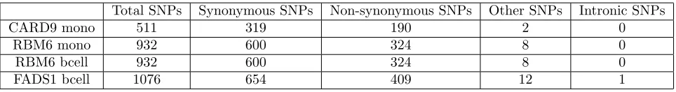
Total SNPs Synonymous SNPs Non-synonymous SNPs Other SNPs Intronic SNPs

CARD9 mono 511 319 190 2 0

RBM6 mono 932 600 324 8 0

RBM6 bcell 932 600 324 8 0

FADS1 bcell 1076 654 409 12 1

Table 4: The number of SNPs in each of the functional information groups for the genes analysed in the Fairfax data.

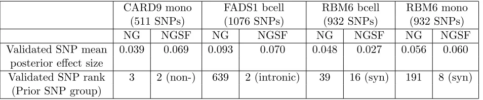
Table 5 shows the the rank and the mean posterior effect size of the validated causal SNP in

0.0

0.2

0.4

0.6

0.8

1.0

0.0 0.2 0.4 0.6 0.8 1.0

T

rue P

ositiv

e Rate (TPR)

False Positive Rate (FPR)

NG splicing

NG

NG UTR

NG mixed

Figure 7: ROCs showing the ranks of the posterior mean effect sizes for 6 causal SNPs in data set 2A for the NG, NG splicing, NG UTR scenarios for n = 300. Five replicate data sets were simulated in HapGen2 [Su et al., 2011] using the LD structure of the CASPASE 8 region in which all the causal SNPs had a MAF of approximately 0.2 in the population. The NG splicing (NG UTR) case is where all 6 causal SNPs are defined as splicing (UTR3) and all 625 non-causal SNPs are from the other 6 functional information groups.

information group that the validated causal SNP belongs to in brackets for the NGSF.

The results in Table 5 convincingly demonstrate that in all cases, including the FADS1 bcell

analysis where the causal SNP is on its own in the intronic group, the rank of the causal SNP has

substantially improved, even though 3 of the validated causal SNPs are neither in the splicing nor

the non-synonymous prior group which represent the groups with a priori less shrinkage. In all

cases the validated SNPS are ranked in the top 2% of SNPs for the NGSF and in 3 out of 4 cases

are ranked in the top 1% of SNPs. For the NG the validated SNPs are in the top 1%, 59%, 4% and

20% of the ranks for the 4 genes considered. This provides convincing evidence that differential

shrinkage based on the SNP group substantively improves detection of the validated SNP in these

CARD9 mono FADS1 bcell RBM6 bcell RBM6 mono

(511 SNPs) (1076 SNPs) (932 SNPs) (932 SNPs)

NG NGSF NG NGSF NG NGSF NG NGSF

Validated SNP mean 0.039 0.069 0.093 0.070 0.048 0.027 0.056 0.060

posterior effect size

Validated SNP rank 3 2 (non-) 639 2 (intronic) 39 16 (syn) 191 8 (syn)

(Prior SNP group)

Table 5: Mean posterior effect size and rank of the single validated SNP in each of 4 genes in the Fairfax data using the NG and the NGSF. For the NGSF we state in brackets whether the the causal SNP is synonymous (syn), non-synonymous (non-syn) or intronic. There are 243 individuals in all analyses.

Discussion

We compared the performance of several currently available multivariate statistical methods, and

one that has never been used before, in fine mapping genes in eQTL studies using simulated

data. Our results showed that using the normal gamma prior assigned higher ranks to simulated

causal SNPs for a given false positive rate. We therefore developed it to allow functional genetic

information to inform the SNP prior effect size with the aim of boosting the rank of causal SNPs.

We applied our new approach to previously published data with validated causal SNPs and observed

considerable increases in the rank of the causal SNP in all four genes tested. We also saw increased

posterior effect size estimates of all simulated causal SNPs compared to the standard NG we choose

to modify. This is primarily due to greater control over the amount of shrinkage enforced. This

is true when all causal SNPs are placed in the same functional group but we have demonstrated

that even when causal SNPs are split across different functional groups, our new method has a

TPR which is never less than that seen in the standard NG. Using the top 1 or 2% of SNPs ranked

by the NGSF for biological validation would lead to a higher chance of detecting the truly causal

SNP than using any other statistical method compared in this paper. Our approach substantially

reduces the risk of not taking forward causal SNPs for validation.

We choose to use the FS score to inform our prior distributions for the causal effect sizes. This

has the advantage of representing information from multiple sources to give a single score. It has

the disadvantage of being bounded by 0 and 1 so that a transformation is required to provide a

prior density with a sufficiently large support to allow meaningful differential shrinkage between

may not need transforming which might lead to Gibbs update and hence faster computing time.

We choose to use empirical priors for the FS scores in the SNP groups. Many of these priors

were mixtures of densities and point masses which led to increased computational complexity.

Using purely continuous priors will likely lead to computational savings. To inform the process of

grouping SNPs, the approach of Pickrell [2014] could be used. In this approach the most relevant

trait-specific annotations are identified via statistical modelling. This method is able to handle

hundreds of genomic annotations without prior knowledge of which are likely to be most relevant.

The approach taken here is to allow the prior effect size to be influenced by functional genomic

information. A possible future avenue of research is to consider the related approach of allowing

functional information to affect the prior inclusion probability of PiMASS [Guan and Stephens,

2011] which is a potentially interesting approach.

Acknowledgements

This work was carried out as part of a PhD project funded by the University of Sheffield. We

would like to thank the reviewers for their constructive comments that markedly improved the

manuscript. The authors have no conflicts of interest to declare.

Appendix - Full conditionals for F for the NGSF

The only full conditional with any substantial change in the NGSF is the full conditional for

F, which isn’t in the standard Normal Gamma prior. Since 2λγ2 _{∼ IG(2, B) it follows that}

π(γ−2|λ, B)∼Ga

2, B

2λ

and since B = tan Fπ₂ǫ+ (1−ǫ) it further follows that

π(γ−2|λ, F) = 1 4λ2_γ2

tanFπ

2ǫ

+ (1−ǫ)2exp −tan F

π

2ǫ

−(1−ǫ) 2λγ2

!

. (17)

All full conditional distributions are calculated using f(F|λ, γ−2) ∝π(F)π(γ−2|λ, F) where π(F)

is the prior distribution on F given in Equations (10) to (16). Metropolis-Hastings acceptance

probabilities are given by

min

1,f(F

′_{|λ, γ}−2₎

f(F|λ, γ−2₎

q(F′, F)

q(F, F′₎

where F′ _{is the proposed value, F is the current value and the form of q(F}′_{, F) depends upon}

whether the proposed value is the point mass from the priors (F∗) in equations (10)-(16) or is

sampled from some suitable probability density.

MCMC updates for _FSyn, FN on−syn and FU T R where the prior is a single density

We first simulateβ according toβ =σ2_{zwherez∼N(0,1) andσ}2 _{is tuned to allow the parameter}

space to be sufficiently explored. Given the current value of F, we then propose F′ according to

F′ =

      

F+ (1−F)Φ(β) if z >0

F−F(1−Φ(β)) if z <0

(19)

It follows from equation(19) that the transition kernel density is

q(F, F′) =

    

φ_σ12Φ−1

F′_−F

1−F

if F′ _{> F}

φ_σ12Φ−1

F′ F

if F′ _{< F.}

(20)

where and φ and Φ are the the standard Gaussian density and distribution function respectively.

Let

T = tan Fπ

2ǫ

+ (1−ǫ), T∗ _{= (T}′_/T)2

T′ _{= tan F}′π

2ǫ

+ (1−ǫ), Q=q(F′_{, F)/q(F, F}′₎

Then using equations (17) and (18) with the priors in equations (12),(15) and (16) it follows that

the acceptance probabilities (AP) are

APFSyn = min   1, QT

∗_expT−T′

2λγ2 

AF

′1.929_exp− F′

0.113

+CF′639.5_{exp −} F

0.0015

AF1.929_{exp −} F

0.113

+CF639.5_{exp −} F

0.0015

    

APFN on−syn = min

1, QT∗_exp

T−T′

2λγ2

APFU T R3 = min

(

1, Q _F′

F 0.45

T∗exp

_{T −T}′

2λγ2 −8.08 (F′−F)

) .

whereA= 0.946

Γ(2.929)0.1132.929 and C= 0.054

MCMC updates for Fintronic, Fintergenic and Fother where the prior is a density and

point mass mixture

We utilize the technique described in Gottardo and Raftery [2004]. This requires that, for the two

measures ν1 and ν2, there exists a measurable set A such that ν1(A) = 0 and ν2(AC) = 0, where AC _{defines the complement of the set A. Formally, we have to exclude the value of the point mass}

from the support of the density to ensure that ν1(A) = 0 and ν2(AC) = 0. Hence the prior is of the formπ(F)∼(1−w)δF∗+wg(F)1_F∈[0,1]\{F∗_} whereF∗ is the value ofF for which there exists

a point mass, wis the mixture proportion andg(F) is the density component of the mixture prior

forF. The procedure is as follows:

1. Let part 1 represent the point mass (1−w)δF∗and part 2 represent the densitywg(F)1F∈[0,1]\{F∗_}.

2. Calculate the component-wise full conditional distributions for F|λ, γ−2 _{for part 1 and part}

2 which depend on the mixing proportion w.

3. Sample a random uniform value u to define which part we sample our proposal value from.

Ifu < p1 we propose the value of the point mass, otherwise we sample a proposal value from

our proposal distribution defined in Equation (19). Note that the value of p1 will need to be

carefully tuned to achieve good chain mixing.

IfF∗ is the value of the point mass,F′ the proposed value then q(F, F′) is given by:

q(F, F′) =

          

p1 if F′ =F∗

(1−p1)φ

1

σ2Φ−1

F′_−F

1−F

if F′ ∈[0,1]\{F∗} and F′ > F

(1−p1)φ

1

σ2Φ−1

F′ F

if F′ _∈[0,1]\{F∗_{} and F}′ _{< F.}

With π(F)∼(1−w)δF∗+wg(F)1_F∈[0,1]\{F∗_}, the general form for the acceptance probability (AP) is AP =                                   

1 ifF =F′ =F∗

min

1, p1wg(F)

(1−w)(1−p1)q(F, F′)

ifF =F∗ _{and F}′ _6=F∗

min

1,(1−w)(1−p1)q(F, F

′₎

p1wg(F)

ifF 6=F∗ _{and F}′ _=F∗

min

1, Qg(F

′₎

g(F)

ifF 6=F∗ and F′ 6=F∗.

(22)

Exact expressions can be derived by substituting the value of w,F∗ and the density component of

the mixture prior g(F), which can be found in equations (10), (11) and (14).

MCMC updates for _Fsplicing where the prior is a mixture of 2 point masses

Here our proposal space is {0,1}. Since q(F, F′) = p1 for both values of F′, the acceptance

probability can be shown to be

APSplicing =

                  

1 ifF =F′

min

1, T∗exp

T −T′

2λγ2

53p1 52(1−p1)

ifF = 0 and F′ = 1

min

1, T∗exp

T −T′

2λγ2

52(1−p1) 53p1

ifF = 1 and F′ = 0.

(23)

References

Altshuler, D. L., Durbin, R. M., Abecasis, G. R., Bentley, D. R., Chakravarti, A., Clark, A. G.,

Collins, F. S., la Vega, F. M. D., Donnelly, P., Egholm, M., et al. (2010). A map of human

genome variation from population-scale sequencing. Nature, 467(7319):1061–1073.

Barrett, J. H., Iles, M. M., Harland, M., Taylor, J. C., Aitken, J. F., Andresen, P. A., Akslen,

L. A., Armstrong, B. K., Avril, M.-F., Azizi, E., et al. (2011). Genome-wide association study

identifies three new melanoma susceptibility loci. Nature Genetics, 43:1108–1113.

Reed, M. W. R., McBurney, H., Latif, A., et al. (2012). Fine-mapping casp8 risk variants in

breast cancer. Cancer Epidemiology Biomarkers and Prevention, 21(1):176–181.

Consortium, E. P. (2011). A user’s guide to the encyclopedia of dna elements (encode). PLoS Biol,

9(4):e1001046.

DeLong, E. R., DeLong, D. M., and Clarke-Pearson, D. L. (1988). Comparing the areas under two or

more correlated receiver operating characteristic curves: a nonparametric approach. Biometrics,

44:837–45.

Fairfax, B. P., Makino, S., Radhakrishnan, J., Plant, K., Leslie, S., Dilthey, A., Ellis, P., Langford,

C., Vannberg, F. O., and Knight, J. C. (2012). Genetics of gene expression in primary immune

cells identifies cell typespecific master regulators and roles of hla alleles. Nature Genetics,

44:502-510.

Gottardo, R. and Raftery, A. E. (2004). Markov chain monte carlo with mixtures of singular

distributions. Journal of Computational and Graphical Statistics, 17(4):949–975.

Griffin, J. E. and Brown, P. J. (2010). Inference with normal-gamma prior distributions in regression

problems. Bayesian Analysis, 5:171–188.

Guan, Y. and Stephens, M. (2011). Bayesian variable selection regression for genome-wide

associ-ation studies and other large-scale problems. The Annals of Applied Statistics, 5:1780–1815.

Hoggart, C. J., Whittaker, J. C., Iorio, M. D., and Balding, D. J. (2008). Simultaneous analysis of

all snps in genome-wide and re-sequencing association studies. PLoS Genetics, 4:e1000130.

Howie, B. N., Donnelly, P., and Marchini, J. (2009). A flexible and accurate genotype imputation

method for the next generation of genome-wide association studies. PLoS Genetics, 5:e1000529.

Ishwaran, H. and Rao, J. S. (2005). Spike and slab variable selection: Frequentist and bayesian

strategies. The Annals of Statistics, 33:730–773.

Kang, G., Lin, D., Hakonarson, H., and Chen, J. (2012). Two-stage extreme phenotype sequencing

design for discovering and testing common and rare genetic variants: Efficiency and power.

Lee, P. H. and Shatkay, H. (2009). An integrative scoring system for ranking snps by their potential

deleterious effects. Bioinformatics, 25:1048–1055.

Lee, S. I., Dudley, A. M., Drubin, D., Silver, P. A., Krogan, N. J., Pe´er, D., and Koller, D. (2009).

Learning a prior on regulatory potential from eqtl data. PLoS Genetics, 5:e1000358.

Mitchell, T. J. and Beauchamp, J. J. (1988). Bayesian variable selection in linear regression.Journal

of the American Statistical Association, 83(404):1023–1032.

Park, T. and Casella, G. (2008). The bayesian lasso.Journal of the American Statistical Association,

103:681–686.

Petersen, A., Alvarez, C., DeClaire, S., and Tintle, N. L. (2013). Assessing methods for assigning

snps to genes in gene-based tests of association using common variants. PLoS ONE, 8(5):e62161.

Pickrell, J. K. (2014). Joint analysis of functional genomic data and genome-wide association

studies of 18 human traits. Am J Hum Genet, 94(4):559–573.

Spencer, A. V., Cox, C., Lin, W.-Y., easton, D.F., Michailidou, K., Walters, K. Incorporating

functional genomic information in genetic association studies using an empirical Bayes approach.

Genet. Epidemiol. In press.

Su, Z., Marchini, J., and Donnelly, P. (2011). Hapgen2: simulation of multiple disease snps.

Bioinformatics.

Wu, M. C., Lee, S., Cai, T., Li, Y., Boehnke, M., and Lin, X. (2011). Rare-variant association

testing for sequencing data with the sequence kernel association test.American Journal of Human