http://eprints.whiterose.ac.uk/104356/
Version: Accepted Version
Article:
Du, H orcid.org/0000-0002-6300-3503 and Alechina, N (2016) Qualitative Spatial Logics
for Buffered Geometries. Journal of Artificial Intelligence Research, 56. pp. 693-745. ISSN
1943-5037
https://doi.org/10.1613/jair.5140
[email protected] https://eprints.whiterose.ac.uk/ Reuse
Unless indicated otherwise, fulltext items are protected by copyright with all rights reserved. The copyright exception in section 29 of the Copyright, Designs and Patents Act 1988 allows the making of a single copy solely for the purpose of non-commercial research or private study within the limits of fair dealing. The publisher or other rights-holder may allow further reproduction and re-use of this version - refer to the White Rose Research Online record for this item. Where records identify the publisher as the copyright holder, users can verify any specific terms of use on the publisher’s website.
Takedown
If you consider content in White Rose Research Online to be in breach of UK law, please notify us by
Qualitative Spatial Logics for Buffered Geometries
Heshan Du [email protected]
University of Leeds, UK
Natasha Alechina [email protected]
University of Nottingham, UK
Abstract
This paper describes a series of new qualitative spatial logics for checking consistency ofsameAs andpartOf matches between spatial objects from different geospatial datasets, especially from crowd-sourced datasets. Since geometries in crowd-sourced data are usu-ally not very accurate or precise, we buffer geometries by a margin of error or a level of toleranceσ∈R≥0, and define spatial relations for buffered geometries. The spatial logics
formalize the notions of ‘buffered equal’ (intuitively corresponding to ‘possibly sameAs’), ‘buffered part of’ (‘possibly partOf’), ‘near’ (‘possibly connected’) and ‘far’ (‘definitely dis-connected’). A sound and complete axiomatisation of each logic is provided with respect to models based on metric spaces. For each of the logics, the satisfiability problem is shown to be NP-complete. Finally, we briefly describe how the logics are used in a system for gen-erating and debugging matches between spatial objects, and report positive experimental evaluation results for the system.
1. Introduction
The motivation for our work on qualitative spatial logics comes from the needs of integrating disparate geospatial datasets, especially crowd-sourced geospatial datasets. Crowd-sourced data involves non-specialists in data collection, sharing and maintenance. Compared to authoritative geospatial data, which is collected by surveyors or other geodata profession-als, crowd-sourced data is less accurate and less well structured, but often provides richer user-based information and reflects real world changes more quickly at a much lower cost (Jackson, Rahemtulla, & Morley, 2010). It is in the interests of national mapping agencies, government organisations, and all other users of geospatial data to be able to integrate and use different geospatial data synergistically.
Figure 1: Prezzo Ristorante and Victoria Shopping Centre represented in OSGB (dotted) and OSM (solid)
In order to integrate the datasets, we need to determine which objects are the same (represent the same entity) and sometimes which objects in one dataset are parts of objects in the other dataset (as in the example of Victoria Shopping Centre). The statements representing these two types of relations are referred to as sameAs matches and partOf matches respectively. One way to produce such matches is to use locations and geometries of objects, although of course we also use any lexical labels associated with the objects, such as names of restaurants etc. In our previous work (Du, Alechina, Jackson, & Hart, 2016), we present a method which generates matches using both location and lexical information about spatial objects. As generated matches may contain errors, they are seen as retractable assumptions and require further validation and checking. One way is to use logical reasoning to check the consistency of matches with respect to statements in input datasets. By using description logic reasoning, the correctness of matches can be checked with respect to classification information. For example, it is wrong to state that spatial objects a and
b are the same, if a is a Bank and b is a Clinic, because the concepts Bank and Clinic
are disjoint, containing no common elements. However, this is not sufficient for validating matches between spatial objects1. For example, two spatial objects which are close to each other in one dataset cannot be matched to two spatial objects which are far away apart in the other dataset, no matter whether they are of the same type or not. Therefore, spatial reasoning is required to validate matches with regard to location information, in addition to description logic reasoning.
Spatial logic studies relations between geometrical structures and spatial languages de-scribing them (Aiello, Pratt-Hartmann, & van Benthem, 2007). There are a variety of spatial relations, such as topological connectedness of regions, relations based on distances, relations for expressing orientations or directions, etc. In a spatial logic, spatial relations are represented in a formal language, such as first order logic or its fragments, and
preted over some structures based on geometrical spaces, such as topological spaces, metric spaces and Euclidean spaces. In the field of qualitative spatial reasoning, several spatial formalisms have been developed for representing and reasoning about topological relations, such as the Region Connection Calculus (RCC) (Randell et al., 1992), the 9-intersection model (Egenhofer & Franzosa, 1991) and their extensions (Clementini & Felice, 1997; Roy & Stell, 2001; Schockaert, Cock, Cornelis, & Kerre, 2008b, 2008a; Schockaert, Cock, & Kerre, 2009). In addition, there are formalisms for representing and reasoning about di-rectional relations (Frank, 1991, 1996; Ligozat, 1998; Balbiani, Condotta, & del Cerro, 1999; Goyal & Egenhofer, 2001; Skiadopoulos & Koubarakis, 2004), as well as relative or absolute distances (Zimmermann, 1995; Clementini, Felice, & Hern´andez, 1997; Wolter & Zakharyaschev, 2003, 2005). Recent comprehensive surveys on qualitative spatial represen-tations and reasoning are provided by Cohn and Renz (2008) and Chen, Cohn, Liu, Wang, OuYang, and Yu (2015).
Qualitative spatial reasoning has been shown to be applicable to geospatial data (Ben-nett, 1996; Ben(Ben-nett, Cohn, & Isli, 1997; Guesgen & Albrecht, 2000; Mallenby, 2007; Mal-lenby & Bennett, 2007; Li, Liu, & Wang, 2013), where location information of spatial objects comes from a single data source. The application described in this paper is differ-ent, as location representations about the same spatial object come from different sources and are usually not exactly the same. Rather than treating all the differences in geometric representations as logical contradictions, we would tolerate slight geometric differences and only treat qualitatively defined ‘large’ differences as logical contradictions used for detecting wrong matches. More specifically, after establishing matches between two sets of spatial objects, if the set of matches gives rise to a contradiction, then some match must be wrong and should be retracted. In addition, we would provide explanations to help users under-stand why a contradiction exists and why some matches are wrong. In the following, we assess the appropriateness of several existing spatial formalisms for these purposes.
The Region Connection Calculus (RCC) (Randell et al., 1992) is a first order formalism based on regions and the connection relation C, which is axiomatised to be reflexive and symmetric. Two regions x, y are connected (i.e. C(x, y) holds), if their closures share a point. Based on the connection relation, several spatial relations are defined for regions. Among them, eight jointly exhaustive and pairwise disjoint (JEPD) relations are identified:
DC(Disconnected),EC(Externally Connected),P O(Partially Overlap),T P P (Tangential Proper Part), N T P P (Non-Tangential Proper Part), T P P i (Inverse Tangential Proper Part), N T P P i (Inverse Non-Tangential Proper Part) and EQ (Equal). They are referred to as RCC8, which is well-known in the field of qualitative spatial reasoning.
The 9-intersection model is developed by Egenhofer and Franzosa (1991) and Egenhofer and Herring (1991) based on the point-set interpretation of geometries. By comparing the nine intersections between interiors, boundaries and exteriors of point-sets, it identifies 29 mutually exclusive topological relations. The 9-intersection model provides a comprehensive formal categorization of binary topological relations between points, lines and regions. Only a small number of these 29 relations are realisable in a particular space (Egenhofer & Herring, 1991). Restricting point-sets to simple regions (regions homeomorphic to disks), the 512 relations collapse to the RCC8 relations.
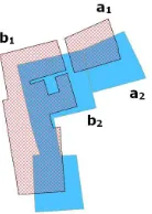
& Franzosa, 1991), since they presuppose accurate geometries or regions with sharp bound-aries and define spatial relations based on the connection relation. This is too strict for crowd-sourced geospatial data. As shown in Figure 2,a1 issameAs a2, both representing a
Prezzo Ristorante;b1 issameAs b2, both referring to a Blue Bell Inn. Though thesameAs
matches are correct, a topological inconsistency still exists, sincea1 andb1 are disconnected (DC), a2 and b2 are externally connected (EC), and the spatial relations DC and EC are
[image:5.612.272.341.213.310.2]disjoint. Therefore, relations based on connection are too strict for crowd-sourced geospatial data which is possibly inaccurate and may contain errors.
Figure 2: In OSGB data, the Prezzo Ristorante (a1) and the Blue Bell Inn (b1) are
discon-nected, whilst in OSM data, they (a2 and b2) are externally connected.
The egg-yolk theory is independently developed by Lehmann and Cohn (1994), Cohn and Gotts (1996b, 1996a), and Roy and Stell (2001) extending the RCC theory and by Clementini and Felice (1996, 1997) extending the 9-intersection model, in order to repre-sent and reason about regions with indeterminate boundaries. In this theory, a region with an indeterminate boundary (an indeterminate region) is represented by a pair of regions, an ‘egg’ and a ‘yolk’, which are the maximum extension and the minimum extension of the indeterminate region respectively (similar to the upper approximation and lower ap-proximation in the rough set theory, Pawlak, Polkowski, & Skowron, 2007). The yolk is not empty and it is always a proper part of the egg. The egg-yolk theory presupposes the existence of a core part of a region and a more vague part. For the described application, the same location can be represented using two disconnected polygons from an authorita-tive geospatial dataset and a crowd-sourced geospatial dataset respecauthorita-tively. In this case, we could not define a certain inner region for any of the disconnected polygons, otherwise, it is inconsistent to treat them as different representations for the same location.
Figure 3: Buffering the geometryX by a distance σ; three dashed circles are buffered part of (BPT) the solid circle; the dashed circle and the solid circle are buffered equal (BEQ)
andEC(a2, b2) = 1, then no contradiction will arise. We did not adopt this approach in the
matching problem, mainly because there is no good way to define the degree of membership, and it is difficult to generate user-friendly explanations for why the matches are wrong if the underlying reasoning is numerical and relatively obscure.
The logic M S(M) was proposed and developed by Sturm, Suzuki, Wolter, and Za-kharyaschev (2000), Kutz, Sturm, Suzuki, Wolter, and ZaZa-kharyaschev (2002), Kutz, Wolter, Sturm, Suzuki, and Zakharyaschev (2003), Wolter and Zakharyaschev (2003, 2005), and Kutz (2007) for reasoning about distances. The logic M S(M) makes it possible to define concepts such as ‘an object within the distance of 100 meters from a School’. M inM S(M) is a parameter set. A typical example ofM isQ≥0. The satisfiability problem for a finite set of M S(Q≥0) formulas in a metric space is EXPTIME-complete (Wolter & Zakharyaschev,
2003). M S(M) was not developed for the problem of geospatial data matching. How-ever, after we designed the logics introduced in this paper, we discovered that they form a proper fragment of M S(Q≥0). To detect problematic matches, we also reason about
dis-tances between objects, but this reasoning is of a more restricted and qualitative kind. The complexity of the satisfiability problem of our logics is NP-complete, which makes them somewhat more suitable for automatic debugging of matches than the full M S(Q≥0). The
syntax and semantics of M S(M) and the proofs for the ‘proper fragment relations’ are provided later in this paper (see Section 3).
In this paper, we present a series of new qualitative spatial logics developed for validating matches between spatial objects: a logic of NEAR and FAR for buffered points (LNF) (Du, Alechina, Stock, & Jackson, 2013), a logic of NEAR and FAR for buffered geometries (LNFS) and a logic of part and whole for buffered geometries (LBPT) (Du & Alechina, 2014a, 2014b). The notion of buffer (ISO Technical Committee 211, 2003) is used to model the uncertainty in geometry representations, tolerating slight differences up to a margin of error or a level of tolerance σ ∈R≥0. As shown in Figure 3, the buffer of a geometry X is
a geometry which contains exactly all the points within σ distance from X. The buffer of
X is denoted asbuffer(X, σ). For a geometryX which is possibly represented inaccurately within the margin of error σ in one dataset, its corresponding representation in the other dataset is assumed to be somewhere withinbuffer(X, σ).
The spatial logics involve four spatial relations BufferedPartOf (BPT), BufferedEqual (BEQ), NEAR and FAR. They formalize the notions of ‘possibly partOf’, ‘possibly sameAs’, ‘possibly connected’ (given a possible displacement by σ) and ‘definitely disconnected’ (even if displaced by σ) respectively. A geometry X is BufferedPartOf a geometry X′, if
Figure 4: NEAR and FAR
each other (Figure 3). We assume that two geometries X and X′ from two diferent datasets may correspond to the same object if they are BufferedEqual. The parameter
σ captures the margin of error in representation of geometries. Two geometries X, Y are NEAR, if the corresponding geometries X′, Y′ in the other dataset could be connected, i.e. distance(X, Y) ∈ [0,2σ] (Figure 4). Clearly, if FAR(X,Y) holds, then NEAR(X,Y) should be false for X and Y from the same dataset. In addition, we want to exclude the possibility that NEAR(X′,Y′) may hold for X′, Y′ (corresponding to X, Y respectively)
in the other dataset. Therefore we define FAR(X,Y) as distance(X, Y) ∈(4σ,+∞) (Fig-ure 4). It is possible that two geometries X, Y are not NEAR and not FAR, this is, distance(X, Y)∈(2σ,4σ].
The way of defining BEQ, N EAR and F AR is similar to that for defining distance relations between points by Moratz and Wallgr¨un (2012), where each point is assigned one or more reference distances. The distance relations between two points X, Y are defined by comparing the distance between X, Y to the reference distances of X and those of Y. As different points can have different reference distances for indicating nearness, distance relations may not be symmetric. Differing from the work by Moratz and Wallgr¨un (2012), the relations we defined are not only for points but also for general geometries, and every geometry has the same reference distances (σ, 2σ and 4σ), which leads to the symmetric definitions of BEQ,N EAR and F AR. We provide sound and complete sets of axioms to support reasoning aboutBEQ,BP T,N EARandF ARrelations (see Section 4). This rea-soning is useful for verifying matches between spatial representations from different sources. As explained in our previous work (Du et al., 2013), though the relations are named
N EAR and F AR, we do not attempt to model human notions of nearness or proximity, which is influenced by several factors, such as absolute distance, relative distance, frame of reference, object size, travelling costs and reachability, travelling distance and attractiveness of objects (Guesgen & Albrecht, 2000). In this work, we provide a strict mathematical definition for the calculation of whether two objects are to be considered as being N EAR
or F AR, based on a margin of error σ. While this makes our approach less likely to be suitable for the simulation of human notions of nearness, it provides a useful tool for verifying consistency of matches. The following arguments are formalized for checking consistency of sameAs and partOf matches: if spatial objects a1, b1 aresameAs orpartOf spatial objects a2, b2 respectively,a1, b1 areN EAR,a2, b2 are F AR, then a contradiction exists.
different geospatial datasets. Section 8 discusses the generality and limitations of the spatial logics. Section 9 concludes the paper.
2. Syntax and Semantics
The language L(LN F) is defined as
φ, ψ:=BEQ(a, b) |N EAR(a, b)|F AR(a, b) | ¬φ|φ∧ψ
where a, b are individual names. φ → ψ ≡def ¬(φ∧ ¬ψ). The language L(LN F S) is
exactly the same asL(LN F). The languageL(LBP T) is almost the same asL(LN F) and
L(LN F S), except that it hasBP T instead ofBEQas a predicate. L(LBP T) is defined as
φ, ψ:=BP T(a, b) |N EAR(a, b)|F AR(a, b) | ¬φ|φ∧ψ.
L(LN F), L(LN F S) and L(LBP T) are all interpreted over models based on a metric space. Every individual name involved in an LNF formula is mapped to a point, whilst each of those involved in an LNFS/LBPT formula is mapped to an arbitrary geometry or a non-empty set of points.
Definition 1 (Metric Space) A metric space is a pair (∆, d), where ∆ is a non-empty set (of points) and d is a metric on ∆, i.e. a function d: ∆×∆ −→ R≥0, such that for any x, y, z ∈∆, the following axioms are satisfied:
1. identity of indiscernibles: d(x, y) = 0 iff x=y;
2. symmetry: d(x, y) =d(y, x);
3. triangle inequality: d(x, z)≤d(x, y) +d(y, z).
Definition 2 (Metric Model of LNF) A metric modelM of LNF is a tuple(∆, d, I, σ), where (∆, d) is a metric space, I is an interpretation function which maps each individual name to an element in ∆, and σ ∈R≥0 is a margin of error. The notion of M |=φ (φ is true in the model M) is defined as follows:
M |=BEQ(a, b) iff d(I(a),I(b))∈[0, σ];
M |=N EAR(a, b) iff d(I(a),I(b))∈[0,2σ];
M |=F AR(a, b) iff d(I(a),I(b))∈(4σ,∞);
M |=¬φ iff M 6|=φ;
M |=φ∧ψ iffM |=φand M |=ψ,
where a, b are individual names, φ, ψ are formulas inL(LN F).
M |=BP T(a, b) iff ∀pa ∈I(a)∃pb ∈I(b) :d(pa,pb)∈[0, σ];
M |=N EAR(a, b) iff ∃pa ∈I(a)∃pb ∈I(b) :d(pa,pb)∈[0,2σ];
M |=F AR(a, b) iff ∀pa ∈I(a)∀pb∈I(b) :d(pa,pb)∈(4σ,∞);
M |=¬φ iff M 6|=φ;
M |=φ∧ψ iffM |=φand M |=ψ,
where a, b are individual names, φ, ψ are formulas in L(LN F S)/L(LBP T). BEQ(a, b) is defined as BP T(a, b)∧BP T(b, a).
The notions of validity and satisfiability in metric models are standard. A formula is satisfiable if it is true in some metric model. A formula φis valid (|=φ) if it is true in all metric models (hence if its negation is not satisfiable). The logic LNF/LNFS/LBPT is the set of all valid formulas in the languageL(LN F)/L(LN F S)/L(LBP T) respectively.
3. Relationship with the logic M S(M)
The logic M S(M), as well as its variations, was developed by Sturm et al. (2000), Kutz et al. (2002, 2003), Wolter and Zakharyaschev (2003, 2005), and Kutz (2007) for reasoning about distances.
M S(M) is a family of logics defined relative to the parameter set M ⊆ Q≥0. M is subject to the following two conditions: if a, b∈M and a+b≤r, then a+b∈M, where
r= supM ifM is bounded, otherwise r=∞; ifa, b∈M and a−b >0, then a−b∈M. The alphabet ofM S(M) consists of
• an infinite list of region variablesX1,X2,...;
• an infinite list of location constants c1,c2,...;
• a set constant{ci} for every location constant ci;
• binary distance (δ), equality (=) and membership (. ∈) predicates;
• the boolean operators⊓,¬ (and their derivatives ⊔,⊤ and⊥);
• two distance quantifiers ∃<a,∃≤a and their duals ∀<a,∀≤a, for everya∈M;
• two universal quantifiers∃ and ∀.
M S(M) terms are defined as:
s, t:=Xi | {ci} | ⊤ | ⊥ | ¬s|s⊓t| ∃<as| ∃≤as| ∃s.
In addition to standard description logic concept constructions, M S(M) can define a concept of objects which are at a distance less thanafrom instances of some other concept
s: ∃<as, and similarly for a distance at most a. ∀<as and ∀≤as are defined as ¬∃<a(¬s)
M S(M) formulas are defined as
φ, ψ:=c∈s|s=. t|δ(c1, c2)< a|δ(c1, c2)≤a| ¬φ|φ∧ψ.
Further, s⊑t is an abbreviation for (s⊓t)=. sand s6=. tis an abbreviation for ¬(s =. t).
δ(c1, c2) > a and δ(c1, c2) ≥ a are defined as¬(δ(c1, c2) ≤a) and ¬(δ(c1, c2) < a) respec-tively.
An M S(M)-modelB is a structure of the form:
B=hW, d, X1B, X2B, ..., cB1, cB2, ...i
where hW, di is a metric space (Definition 1), each XB
i is a subset of W, and each cBi is
an element of W. The value of any other M S(M)-term in B is computed inductively as follows:
• ⊤B=W,⊥B=∅;
• {ci}B ={cBi };
• (¬s)B =W −sB;
• (s1⊓s2)B =sB1 ∩sB2;
• (∃<as)B={x∈W | ∃y ∈sB:d(x, y)< a};
• (∃≤as)B={x∈W | ∃y ∈sB:d(x, y)≤a};
• (∃s)B ={x∈W | ∃y∈sB}.
∀<a,∀≤a and ∀ are dual to∃<a,∃≤a and ∃respectively. For instance,
(∀<as)B={x∈W | ∀y∈W : (d(x, y)< a→y∈sB)}.
The truth condition of B |=φ, whereφis an M S(M)-formula, is defined as follows:
• B |=c∈siff cB∈sB;
• B |=s1 =. s2 iffsB1 =sB2;
• B |=δ(k, l)< a iffd(kB, lB)< a;
• B |=δ(k, l)≤aiffd(kB, lB)≤a;
• B |=¬φiffB 6|=φ;
• B |=φ∧ψiff B |=φand B |=ψ.
A set of M S(M) formulas Σ is satisfiable, if there exists an M S(M)-model B such that
B |=φfor everyφ∈Σ. This is denoted asB |= Σ.
It is proved below that LNF/LNFS/LBPT are proper fragments of the logicM S(Q≥0).
Lemma 1 For individual names a, b, the M S(M) formula {a} ⊑ ¬{b} is not expressible in LNF.
Proof. Let M1, M2 be metric models2. M1= (∆1, d, I1, σ), M2= (∆2, d, I2, σ).
In M1, ∆1 ={o1, o2},d(o1, o2) =σ. I1(a) =o1,I1(b) =o2. For any individual name x
differing from a, b,I1(x) =o1.
In M2, ∆2 ={o}. I2(a) = o, I2(b) = o. For any individual name x differing from a, b, I2(x) =o. For any individual name y,Ii({y}) ={Ii(y)},i∈ {1,2}.
By the definitions of M1, M2, for any individual names x, y, d(I1(x), I1(y)) ∈ [0, σ], d(I2(x), I2(y)) = 0. Ifφis an atomic LNF formula aboutx, y, then by Definition 2,M1|=φ
iff M2 |=φ. By an easy induction on logical connectives, for any LNF formula φ, M1 |=φ
iff M2 |=φ.
Since I1({a}) ={o1}, I1({b}) ={o2} and I2({a}) =I2({b}) ={o}, by the truth
defini-tion of M S(M) formulas, M1 |= ({a} ⊑ ¬{b}),M2 6|= ({a} ⊑ ¬{b}). Hence,{a} ⊑ ¬{b} is not equivalent to any LNF formula.
Lemma 2 The logic LNF is a proper fragment of the logic M S(Q≥0).
Proof. Every atomic LNF formula is expressible in M S(Q≥0):
• BEQ(a, b)≡(δ(a, b)≥0)∧(δ(a, b)≤σ);
• N EAR(a, b)≡(δ(a, b)≥0)∧(δ(a, b)≤2σ);
• F AR(a, b)≡(δ(a, b)>4σ).
This means that all LNF formulas can be expressed in a fragment ofM S(Q≥0) (the image
of LNF under the translation above) which only contains location constants, binary dis-tance predicate and boolean connectives ¬,∧. By Lemma 1, LNF is a proper fragment of
M S(M).
Lemma 3 For individual names a, b, the M S(M) formula a ⊑ ¬b is not expressible in LNFS/LBPT.
Proof. Let M1, M2 be metric models3. M1= (∆1, d, I1, σ), M2= (∆2, d, I2, σ).
In M1, ∆1 = {o1, o2}, d(o1, o2) = σ. I1(a) = {o1}, I1(b) = {o2}. For any individual
name xdiffering from a, b,I1(x) ={o1}.
In M2, ∆2 ={o}. I2(a) ={o},I2(b) ={o}. For any individual name x differing from a, b,I2(x) ={o}.
If φ is an atomic LNFS/LBPT formula about x, y, then by Definition 3, M1 |= φ iff M2 |= φ. By an easy induction on logical connectives, for any LNFS/LBPT formula φ, M1 |=φiffM2 |=φ.
2. Note that we can construct models in a one-dimensional or two-dimensional Euclidean space in a similar way and prove the lemma.
By the truth definition of M S(M) formulas, M1 |= (a ⊑ ¬b) and M2 6|= (a ⊑ ¬b).
Hence,a⊑ ¬bis not equivalent to any LNFS/LBPT formula.
Lemma 4 The logic LNFS/LBPT is a proper fragment of M S(Q≥0).
Proof. Every atomic LNFS/LBPT formula is expressible in M S(Q≥0):
• (For LNFS) BEQ(a, b) iff (a⊑(∃≤σb))∧(b⊑(∃≤σa));
• (For LBPT)BP T(a, b) iff (a⊑(∃≤σb));
• N EAR(a, b) iff (a⊓(∃≤2σb)6=. ⊥);
• F AR(a, b) iff (a⊓(∃≤4σb)=. ⊥).
Note that the formulas on the right belong to a fragment of M S(Q≥0) which is the image of LNFS/LBPT under the translation above.
The correctness of translation of BEQ(a, b) and BP T(a, b) into M S(Q≥0) follows
di-rectly from the truth definition of BEQ andBP T (Definition 3). To show that the trans-lation of N EAR and F AR are correct, consider that the truth definition of N EAR(a, b) is equivalent to 0≤dmin(a, b)≤2σ and F AR(a, b) to dmin(a, b)>4σ, where dmin(a, b) =
inf{d(pa, pb)|pa∈I(a), pb ∈I(b)}. It was shown by Wolter and Zakharyaschev (2005) that dmin(a, b) ≤ m iff a⊓(∃≤mb) 6=. ⊥. This makes the translation of the formulas have the
same truth conditions as defined in Definition 3. By Lemma 3, LNFS/LBPT is a proper fragment of M S(Q≥0).
Wolter and Zakharyaschev (2003) proved that the satisfiability problem for a finite set of M S(Q≥0) formulas in a metric space is EXPTIME-complete, which provides an upper
bound on the complexity of the satisfiability problems of LNF, LNFS and LBPT in a metric space.
Kutz et al. (2002) and Kutz (2007) gave axioms or inference rules connecting M S(M) terms (e.g. ∀≤0s → s) for M S(M) and its variants. However, the axiomatisation we are
going to present is for LNF, LNFS and LBPT formulas (corresponding toM S(M) formulas rather thanM S(M) terms).
4. Axioms and Theorems
This section presents a sound and complete axiomatisation for the logic LNF/LNFS/LBPT respectively. The axiomatic systems have been used as a basis for a rule-based reasoner described later in Section 7 4.
The following calculus (which we will also refer to as LNF) is sound and complete for LNF:
Axiom 0 All tautologies of classical propositional logic
Axiom 1 BEQ(a, a);
Axiom 2 BEQ(a, b)→BEQ(b, a);
Axiom 3 N EAR(a, b)→N EAR(b, a);
Axiom 4 F AR(a, b)→F AR(b, a);
Axiom 5 BEQ(a, b)∧BEQ(b, c)→N EAR(c, a);
Axiom 6 BEQ(a, b)∧N EAR(b, c)∧BEQ(c, d)→ ¬F AR(d, a);
Axiom 7 N EAR(a, b)∧N EAR(b, c)→ ¬F AR(c, a);
MP Modus ponens: φ, φ→ψ ⊢ ψ.
The following calculus (which we will also refer to as LNFS) is sound and complete for LNFS:
Axiom 0 All tautologies of classical propositional logic
Axiom 1 BEQ(a, a);
Axiom 2 BEQ(a, b)→BEQ(b, a);
Axiom 3 N EAR(a, b)→N EAR(b, a);
Axiom 4 F AR(a, b)→F AR(b, a);
Axiom 5 BEQ(a, b)∧BEQ(b, c)→N EAR(c, a);
Axiom 6 BEQ(a, b)∧N EAR(b, c)∧BEQ(c, d)→ ¬F AR(d, a);
Axiom 8 N EAR(a, b)∧BEQ(b, c)∧BEQ(c, d)→ ¬F AR(d, a);
MP Modus ponens: φ, φ→ψ ⊢ ψ.
Axiom 7 of the calculus LNF only holds for points, but not for arbitrary geometries, because two points within the same line or polygon can be far from each other. Axiom 7 is replaced by Axiom 8 in LNFS. All other axioms in LNFS are the same as those in LNF.
The following calculus (which we will also refer to as LBPT) is sound and complete for LBPT:
Axiom 0 All tautologies of classical propositional logic
Axiom 3 NEAR(a,b)→NEAR(b,a);
Axiom 4 FAR(a,b)→FAR(b,a);
Axiom 9 BPT(a,a);
Axiom 11 BPT(b,a)∧BPT(b,c)→NEAR(c,a);
Axiom 12 BPT(b,a)∧NEAR(b,c)∧BPT(c,d)→ ¬FAR(d,a);
Axiom 13 NEAR(a,b)∧BPT(b,c)∧BPT(c,d)→ ¬FAR(d,a);
MP Modus ponens: φ, φ→ψ ⊢ ψ.
The calculus LBPT is similar to the calculus LNFS. Changing predicates from BEQ to
BP T, LNFS Axioms 1, 6, 8 are replaced by Axioms 9, 12, 13 respectively in LBPT. Since
BP T is not symmetric, LNFS Axiom 2 does not have a corresponding axiom in LBPT, and LNFS Axiom 5 is replaced by two LBPT axioms, Axiom 10 and Axiom 11.
The notion of derivability Γ⊢φin LNF/LNFS/LBPT calculus is standard. A formula
φ is derivable if ⊢ φ. A set Γ is LNF/LNFS/LBPT-inconsistent if for some formula φ it derives bothφ and¬φ.
We proved the following theorems for LNF, LNFS and LBPT.
Theorem 1 (Soundness and Completeness) The LNF/LNFS/LBPT calculus is sound and complete for metric models, namely that
⊢φ ⇔ |=φ
(every derivable formula is valid and every valid formula is derivable).
Theorem 2 (Decidability and Complexity) The satisfiability problem for a finite set of LNF/LNFS/LBPT formulas in a metric space is NP-complete.
In the following sections, we give proofs of the results above for the case of LBPT. The proofs for LNF and LNFS are similar. For LBPT, we have the following derivable formulas, which we will refer to as facts in the completeness proof:
Fact 14 BP T(a, b)→N EAR(a, b);
Fact 15 N EAR(a, b)→ ¬F AR(a, b);
Fact 16 N EAR(a, b)∧BP T(b, c)→ ¬F AR(c, a);
Fact 17 BP T(a, b)→ ¬F AR(a, b);
Fact 18 BP T(a, b)∧BP T(b, c)→ ¬F AR(c, a);
Fact 19 BP T(b, a)∧BP T(b, c)→ ¬F AR(c, a);
Fact 20 BP T(a, b)∧BP T(b, c)∧BP T(c, d)→ ¬F AR(d, a);
Fact 21 BP T(b, a)∧BP T(b, c)∧BP T(c, d)→ ¬F AR(d, a);
Fact 22 BP T(a, b)∧BP T(b, c)∧BP T(c, d)∧BP T(d, e)→ ¬F AR(e, a);
Fact 23 BP T(b, a)∧BP T(b, c)∧BP T(c, d)∧BP T(d, e)→ ¬F AR(e, a);
Fact 24 BP T(b, a)∧BP T(c, b)∧BP T(c, d)∧BP T(d, e)→ ¬F AR(e, a).
5. Soundness and Completeness of LBPT
This section shows that the LBPT calculus is sound and complete for metric models. Though several definitions and lemmas have been presented in our previous work (Du et al., 2013; Du & Alechina, 2014b), the proofs presented here are more complete, structured, ac-curate (small errors are corrected) and simplified.
The proof of soundness (every LBPT derivable formula is valid: ⊢ φ⇒ |=φ) is by an easy induction on the length of the derivation of φ. Axioms 3, 4, 9-13 are valid (by the truth definition ofBP T,N EARand F AR) and modus ponens preserves validity.
In the rest of this section, we prove completeness (every LBPT valid formula is deriv-able):
|=φ⇒ ⊢φ
We will actually prove that if a finite set of LBPT formulas Σis consistent, then there is a metric model satisfying it. Any finite set of formulas Σ can be rewritten as a formula
ψ which is the conjunction of all formulas in Σ. Σ is consistent, iffψ is consistent (6⊢ ¬ψ). If there is a metric model M satisfying Σ, then M satisfies ψ, thus 6|= ¬ψ. Therefore, if we show that if Σ is consistent, then there exists a metric model satisfying it, then we show that if 6⊢ ¬ψ, then 6|= ¬ψ. This shows that6⊢ φ⇒6|=φ and by contraposition we get completeness.
The completeness theorem is proved by constructing a metric model for a maximal consistent set (Definition 4) of any finite consistent set of LBPT formulas (Lemma 5).
Definition 4 (MCS) A set of formulas Γ in the language L(LBP T) is maximal consis-tent, ifΓis consistent, and any set of LBPT formulas over the same set of individual names properly containing Γ is inconsistent. If Γis a maximal consistent set of formulas, then we call it an M CS.
Proposition 1 (Properties of MCSs) If Γ is anM CS, then,
• Γ is closed under modus ponens: ifφ, φ→ψ∈Γ, then ψ∈Γ;
• if φis derivable, then φ∈Γ;
• for all formulas φ: φ∈Γ or ¬φ∈Γ;
• for all formulas φ, ψ: φ∧ψ∈Γ iff φ∈Γ and ψ∈Γ;
• for all formulas φ, ψ: φ∨ψ∈Γ iff φ∈Γ or ψ∈Γ.
Lemma 5 (Lindenbaum’s Lemma) If Σ is a consistent set of formulas in the language
L(LBP T), then there is an M CS Σ+ over the same set of individual names such that Σ⊆Σ+.
Letφ0, φ1, φ2, ...be an enumeration of LBPT formulas over the same set of individual names
as that in Σ. Σ+ can be defined as follows:
• Σ0= Σ;
• Σ+=S
n≥0Σn.
For a finite consistent set of formulas Σ, we construct a metric model satisfying a maximal consistent set Σ+, which contains Σ and is over the same set of individual names
as Σ, as follows. Firstly, we equivalently transform Σ+ toB(Σ+), which is a set of basic quantified formulas. Then we construct a set of distance constraints D(Σ+) from B(Σ+). A key concept here is path-consistency for a set of distance constraints.
Definition 5 (Non-negative Interval) An interval h is non-negative, if h ⊆ [0,+∞).
Definition 6 (Distance Constraint, Distance Range) A distance constraint is a state-ment of the form d(p, q)∈g, wherep, q are constants representing points,d(p, q) stands for the distance between p, q, and g is a non-negative interval, which stands for the distance range for p, q.
Definition 7 (Composition) If d1, d2 are non-negative real numbers, then the composi-tion of {d1} and {d2} is defined as: {d1} ◦ {d2} = [|d1−d2|, d1+d2] 5. If g1, g2 are non-negative intervals, then their composition is an interval which is the union of all{d1}◦{d2}, where d1∈g1, d2∈g2, this is,
g1◦g2 =Sd1∈g1,d2∈g2{d1} ◦ {d2}.
It is assumed that a set of distance constraintsDcontains at most one distance range for each pair of constantsp, q involved inD, andDis closed under symmetry, i.e. ifd(p, q)∈g
is in D, thend(q, p)∈g is in D.
Definition 8 (Path-Consistency) For a set of distance constraints D, for every pair of different constants p, q involved in D, their distance range is strengthened by successively applying the following operation until a fixed point is reached:
∀s:g(p, q)←g(p, q)∩(g(p, s)◦g(s, q))
where s is a constant in D, s 6= p, s6= q, and g(p, q) denotes the distance range for p, q. This process is called enforcing path-consistency on D. If at a fixed point, for every pair of constants p, q, g(p, q)6=∅, then D is called path-consistent.
In this paper, we say an interval is referred to in the process of enforcing path-consistency onD, if it occurs inDor is involved in the enforcement of the operationg(p, q)←g(p, q)∩ (g(p, s)◦g(s, q)). In other words, it is used asg(p, q),g(p, s) org(s, q). A distance constraint appears in the process of enforcing path-consistency onD, if its distance range (an interval) is referred to in the process of enforcing path-consistency onD.
The way of enforcing path-consistency on a set of distance constraints defined above is almost the same as that of enforcing path-consistency on a binary constraint satisfaction problem (CSP) (Renz & Nebel, 2007; van Beek, 1992), except that the operation ∀s :
g(p, q)←g(p, q)∩(g(p, s)◦g(s, q)) (◦is the composition operator for non-negative intervals, Definition 7) is applied instead of∀k:Rij ←Rij∩(Rik◦Rkj) (◦is the composition operator
for relations). The time complexity of the path-consistency algorithm for CSP isO(n3) (van Beek, 1992; Mackworth & Freuder, 1985), where n is the number of variables involved in the input set of binary constraints. The path-consistency algorithm for CSP can be adapted easily for enforcing path-consistency on a set of distance constraints. The time complexity of the resulting path-consistency algorithm is alsoO(n3), wherenis the number of constants involved in the input set of distance constraints. Later in this paper, we will show that the process of enforcing path-consistency on D(Σ+) terminates, and a fixed point can be
reached in O(n3) (see Lemma 33).
After constructing a set of distance constraints D(Σ+) from Σ+, we prove the Metric Model Lemma, Metric Space Lemma and Path-Consistency Lemma which are stated below. The notion of path-consistency acts as a bridge between the lemmas.
Lemma 6 (Metric Model Lemma) Let Σbe a finite consistent set of formulas, andΣ+ be an M CS which contains Σ and is over the same set of individual names as Σ. If a metric space satisfies D(Σ+), then it can be extended to a metric model satisfyingΣ+.
Lemma 7 (Metric Space Lemma) Let Σ be a finite consistent set of formulas, and Σ+ be anM CS which contains Σand is over the same set of individual names as Σ. IfD(Σ+) is path-consistent, then there is a metric space (∆, d) such that all distance constraints in
D(Σ+) are satisfied.
Lemma 8 (Path-Consistency Lemma) LetΣbe a finite consistent set of formulas, and Σ+ be anM CSwhich contains Σand is over the same set of individual names asΣ. Then,
D(Σ+) is path-consistent.
Using these three lemmas, we prove the completeness of LBPT: if a finite set of formulas Σ is LBPT-consistent, then there exists a metric model satisfying it.
Proof. If Σ is LBPT-consistent, by the Lindenbaum’s Lemma (Lemma 5), there is anM CS
Σ+ over the same set of individual names such that Σ ⊆ Σ+. By the Path-Consistency Lemma (Lemma 8) and the Metric Space Lemma (Lemma 7), there is a metric space (∆, d) such that all distance constraints in D(Σ+) are satisfied. By the Metric Model Lemma (Lemma 6), the metric space can be extended to a metric model M satisfying Σ+. Since Σ⊆Σ+,M satisfies Σ.
The detailed proofs of the Metric Model Lemma, Metric Space Lemma and Path-Consistency Lemma are provided in Section 5.1, Section 5.2 and Section 5.3 respectively. Note that, in this paper, Σ+ denotes anM CS which contains a given finite consistent set of formulas Σ and is over the same set of individual names as Σ.
5.1 Metric Model Lemma
This section shows how to construct a set of distance constraints D(Σ+) from Σ+, and presents the proof of the Metric Model Lemma.
Lemma 9 If Σ+ is an M CS, then for any pair of individual names a, b occurring in Σ, exactly one of the following cases holds in Σ+:
1. case(a, b) =BP T(a, b)∧BP T(b, a);
2. case(a, b) =BP T(a, b)∧ ¬BP T(b, a);
3. case(a, b) =¬BP T(a, b)∧BP T(b, a);
4. case(a, b) =¬BP T(a, b)∧ ¬BP T(b, a)∧N EAR(a, b);
5. case(a, b) =¬N EAR(a, b)∧ ¬F AR(a, b);
6. case(a, b) =F AR(a, b),
where case(a, b) denotes the formula which holds betweena, b in each case.
Lemma 9 is proved using LBPT axioms and facts (such as Axiom 3, Facts 14, 15) in the same way as proving the lemma for LNF (see Du et al., 2013). The full proof of Lemma 9 is provided in Appendix A.
The construction of a set of distance constraintsD(Σ+) from Σ+ has two main steps:
Step 1 For every pair of individual namesa, b occurring in Σ, we translatecase(a, b) into a set of first order formulas which is equi-satisfiable to case(a, b). The union of all such sets of first order formulas isB(Σ+) (hence,B(Σ+) and Σ are equi-satisfiable.).
This step is described by Definition 9 and Definition 10.
Step 2 We construct a set of distance constraints D(Σ+) from B(Σ+). This step is de-scribed by Definitions 11-13.
For LBPT formulas, there are first order formulas corresponding to their truth definition in Definition 3. We use formulas of the formd(p, q)∈gas abbreviations of their equivalent first order formulas. For example, d(p, q) ∈ [0, σ] abbreviates d(p, q) ≥ 0∧d(p, q) ≤ σ. Observe that6
• BP T(a, b) and ∀pa ∈a ∃pb ∈b :d(pa,pb)∈[0, σ] are equi-satisfiable ;
• N EAR(a, b) and ∃pa ∈a ∃pb ∈b:d(pa,pb)∈[0,2σ] are equi-satisfiable;
• F AR(a, b) and∀pa ∈a ∀pb ∈b:d(pa,pb)∈(4σ,∞) are equi-satisfiable.
Definition 9 (Basic Quantified Formula) We refer to the first order formulas of the following forms as basic quantified formulas:
• ∀pa ∈a ∀pb ∈b:d(pa,pb)∈g;
• ∃pa ∈a ∃pb ∈b:d(pa,pb)∈g;
6. Note that by ∀pa∈a∃pb∈b:d(pa,pb)∈[0, σ], we are actually quantifying over a metric space. In such sense, it is more precise to say, for example, BP T(a, b) is satisfiable in a metric model, iff
• ∀pa ∈a ∃pb ∈b:d(pa,pb)∈g;
• ∃pa ∈a ∀pb ∈b:d(pa,pb)∈g,
where g is a non-negative interval. The abbreviations of these four forms are defined as ∀(a, b, g), ∃(a, b, g), χ(a, b, g) and ξ(a, b, g) respectively. In other words, for example, ∀(a, b, g)≡(∀pa ∈a ∀pb ∈b:d(pa,pb)∈g).
Now we translate the formula in each case listed in Lemma 9 into basic quantified formulas, which will be used to count the number of points needed for interpreting individual names occurring in Σ later.
Definition 10 (B(Σ+)) For anM CS Σ+ over the same set of individual names asΣ, its corresponding set of basic quantified formulas B(Σ+) is constructed as follows. For every pair of individual names a, b, we translate case(a, b) into basic quantified formulas:
• translate(BP T(a, b)∧BP T(b, a)) ={χ(a, b,[0, σ]), χ(b, a,[0, σ])};
• translate(BP T(a, b)∧ ¬BP T(b, a)) ={χ(a, b,[0, σ]), ξ(b, a,(σ,∞))};
• translate(¬BP T(a, b)∧BP T(b, a)) ={ξ(a, b,(σ,∞)), χ(b, a,[0, σ])};
• translate(¬BP T(a, b)∧ ¬BP T(b, a)∧N EAR(a, b)) ={ξ(a, b,(σ,∞)), ξ(b, a,(σ,∞)),∃(a, b,[0,2σ]),∃(b, a,[0,2σ])};
• translate(¬N EAR(a, b)∧ ¬F AR(a, b)) ={∀(a, b,(2σ,∞)),∀(b, a,(2σ,∞)),
∃(a, b,[0,4σ]),∃(b, a,[0,4σ])};
• translate(F AR(a, b)) ={∀(a, b,(4σ,∞)),∀(b, a,(4σ,∞))},
where σ ∈ R≥0 is a fixed margin of error. Let names(Σ) be the set of individual names occurring in Σ. Then,
B(Σ+) =S
a∈names(Σ),b∈names(Σ)translate(case(a, b)).
In the following, for a set of basic quantified formulas B(Σ+), we construct a set of
distance constraintsD(Σ+), and then show that if there is a metric space satisfyingD(Σ+), then it can be extended to a model of Σ+. In other words, we are constructing a metric
over a set of points used to interpret individual names.
The number of points needed for interpreting each individual name depends on the numbers of different forms of formulas inB(Σ+). For any individual name a, let us predict how many particular constants inpoints(a) (points assigned to an individual namea) can be specified by the finite set of formulas about a in B(Σ+). points(a) contains at least one constant. If a formula in B(Σ+) says ‘there exists a constant in points(a)’, then this constant is a particular constant withinpoints(a). For any pair of different individual names
a, b, if both ∃(a, b, g) and ∃(b, a, g) are in B(Σ+), we only count one of them; if χ(a, b, g) is inB(Σ+), we map all the constants in points(a) to the same constant in points(b). By Lemma 9 and Definition 10, in B(Σ+), for any pair of different individual names a, b and R ∈ {∃, ξ, χ} we never have R(a, b, g1) and R(a, b, g2), where g1 6= g2, at the same time.
Definition 11 (num(a, B(Σ+)) and points(a)) Letnames(Σ)be the set of individual names occurring in Σ 7. For any individual namea∈names(Σ),
num(∃a,B(Σ+)) =|{b ∈names(Σ)| ∃g:∃(a,b,g)∈B(Σ+)}| num(ξa,B(Σ+)) =|{b ∈names(Σ)| ∃g:ξ(a,b,g)∈B(Σ+)}| num(χa,B(Σ+)) =|{b ∈names(Σ)| ∃g:χ(b,a,g)∈B(Σ+)}|
Then num(a,B(Σ+)) =num(∃a,B(Σ+)) +num(ξa,B(Σ+)) +num(χa,B(Σ+)).
points(a) is a set of constants {p1a, . . . , pan}, where n=num(a, B(Σ+)).
Definition 12 (Witness for a formula) A witness for a formula ∃(a, b, g) is a pair of constants pa ∈ points(a), pb ∈points(b) such that d(pa, pb) ∈g. A witness for a formula ξ(a, b, g)orχ(b, a, g)is a constantpa∈points(a), such that for any constantpb ∈points(b), d(pa, pb)∈g. A constant is clean for a formula, if it is not a witness for any other formula.
Definition 13 (D(Σ+)) Let B(Σ+) be the corresponding set of basic quantified formulas of an M CS Σ+. For every individual name a in Σ, we assign a fixed set of new con-stants points(a) to it. We construct a set of distance constraints D(Σ+) as follows, by iterating through the basic quantified formulas inB(Σ+) and eliminating quantifiers on new constants. Initially, D(Σ+) = {}. For every individual name a in Σ, for every constant pa ∈ points(a), we add d(pa, pa) ∈ {0} to D(Σ+). For every pair of different individual names a, b, if
• ∃(a,b,g)∈B(Σ+), then we take clean constants pa ∈points(a), pb ∈points(b), and
add d(pa,pb) =d(pb,pa)∈g toD(Σ+), so pa, pb become a witness for ∃(a,b,g);
• ξ(a,b,g)∈B(Σ+), then we take a clean constant pa ∈points(a), for every pb ∈points(b),
we add d(pa,pb) =d(pb,pa)∈g toD(Σ+), so pa becomes a witness forξ(a,b,g);
• ξ(b,a,g)∈B(Σ+), then we take a clean constant pb ∈points(b), for every pa ∈points(a),
we add d(pa,pb) =d(pb,pa)∈g toD(Σ+), so pb becomes a witness forξ(b,a,g);
• χ(a,b,g)∈B(Σ+), then we take a clean constant pb ∈points(b), for every pa∈points(a),
we add d(pa,pb) =d(pb,pa)∈g toD(Σ+), so pb becomes a witness forχ(a,b,g);
• χ(b,a,g)∈B(Σ+), then we take a clean constant pa ∈points(a), for every pb ∈points(b),
we add d(pa,pb) =d(pb,pa)∈g toD(Σ+), so pa becomes a witness forχ(b,a,g);
• ∀(a,b,g)∈B(Σ+), then for every pair of constants pa ∈points(a), pb ∈points(b),
we add d(pa,pb) =d(pb,pa)∈g toD(Σ+).
For every pair of different constants p, q in D(Σ+), we add d(p,q) =d(q,p) ∈[0,∞) to D(Σ+), then repeatedly replace d(p,q) =d(q,p)∈g
1 and d(p,q) =d(q,p)∈g2 with
d(p,q) =d(q,p)∈(g1∩g2), until there is only one distance range for each pair of p, q in D(Σ+).
In Definition 13, for every pair of different individual names a, b, we check whether
χ(a,b,g)∈B(Σ+) holds and check whether χ(b,a,g)∈B(Σ+) holds, because it is pos-sible only one of them holds. For the same reason, we check ξ(a,b,g)∈B(Σ+) and
ξ(b,a,g)∈B(Σ+) separately. By Definition 10, ∃(a,b,g)∈B(Σ+) iff ∃(b,a,g)∈B(Σ+).
Hence we only need to check any one of them. We only check whether∀(a,b,g)∈B(Σ+) holds, as∀(a,b,g)∈B(Σ+) iff∀(b,a,g)∈B(Σ+).
Lemma 10 When constructing D(Σ+), for any individual name a, the number of clean constants needed frompoints(a) is no larger than num(a, B(Σ+)).
Proof. By Definition 10, for any individual namea,χ(a, a,[0, σ]) is in B(Σ+). By Defini-tion 11,num(a, B(Σ+))≥1.
If a is not involved in any formula of the form ∃(a, b, g), ξ(a, b, g) or χ(b, a, g), for any other individual name b, then by Definition 11, num(a, B(Σ+)) = 1. By Definition 13, we need no clean constants from points(a).
Otherwise, by Lemma 9 and Definition 10, inB(Σ+), for any pair of different individual namesa, bandR∈ {∃, ξ, χ}, we never haveR(a, b, g1) andR(a, b, g2), whereg16=g2, at the same time. By Definition 13, for each ∃(a, b, g)∈B(Σ+), we take one clean constant from points(a), so num(∃a, B(Σ+)) clean constants are needed in total for all formulas of this form. Similarly, num(ξa, B(Σ+)) and (num(χa, B(Σ+))−1) clean constants are needed for formulas of formsξ(a, b, g) andχ(b, a, g) respectively, where a, baredifferent individual names. We do not need any other clean constant frompoints(a) for formulas in other forms. By Definition 11,num(a, B(Σ+)) is enough.
D(Σ+) andB(Σ+) are not equi-satisfiable because of the way we assign witnesses for χ
formulas. More specifically, for any pair of different individual namesa, b, if χ(a, b, g) is in
B(Σ+), we map all the constants in points(a) to the same constant in points(b). In other
words, if B′(Σ+) is the set of formulas resulting from replacing every χ(a, b, g) in B(Σ+) withξ(b, a, g), thenD(Σ+) andB′(Σ+) are equi-satisfiable. Since every individual name is
interpreted as a non-empty set of constants, if a model satisfies ξ(b, a, g), then it satisfies
χ(a, b, g), but not vice versa. Hence, constructing D(Σ+) for B′(Σ+) rather than B(Σ+) imposes stronger restrictions (i.e. χ(a, b, g) inB(Σ+) is replaced with ξ(b, a, g) inB′(Σ+))
on the metric space compared to that required by Σ+. However, later we will show that
if Σ+ is consistent, then D(Σ+) can be satisfied in a metric space by proving the Metric Space Lemma and Path-Consistency Lemma in the following sections.
Before proving the Metric Model Lemma, let us look at some important properties of
D(Σ+), as shown by Lemmas 11-13. The proof of Lemma 11 is provided in Appendix A. Lemma 12 follows from the proof of Lemma 11.
Lemma 11 For any distance rangeg occurring in D(Σ+),
g∈ {{0},[0, σ],(σ,∞),[0,2σ],(2σ,∞),(2σ,4σ],(4σ,∞),[0,∞)}.
Lemma 12 Ifp∈points(a), q∈points(b), anda6=b, thend(p, q)∈ {0} is not inD(Σ+).
Proof. It is assumed that Σ is a finite consistent set of formulas over n (a finite num-ber) individual names. By Lemma 9 and Definition 10, B(Σ+) contains at most f = (n+ 2n(n−1)) formulas over n individual names. By Definition 11, for any individual name a, num(a, B(Σ+)) ≤ f. By Definition 13, the number of constants in D(Σ+) is at
mostnf.
The Metric Model Lemma is proved as follows.
Lemma 14 If a metric model satisfies B(Σ+), then it satisfies Σ+.
Proof. The lemma follows from two observations. First, by Lemma 9, Σ+ is entailed by the setC(Σ+) ={case(a, b) :a∈names(Σ+), b∈names(Σ+)}. Second, by Definition 10,
B(Σ+) is a translation of truth conditions ofC(Σ+) into first order logic. If a metric model
satisfiesB(Σ+), then it satisfies C(Σ+), and hence it satisfies Σ+.
Lemma 6 (Metric Model Lemma) Let Σ be a finite consistent set of formulas, and Σ+ be an M CS which contains Σ and is over the same set of individual names asΣ. If a metric space satisfies D(Σ+), then it can be extended to a metric model satisfyingΣ+.
Proof. Suppose a metric space satisfies D(Σ+). We extend it to a metric model M by
interpreting every individual name a occurring in Σ+ as points(a), a’s corresponding set of constants of size num(a, B(Σ+)) (Definition 11 and Definition 13). By Definition 13, any formula of the form χ(a, a,[0, σ]) is satisfied by M. For any pair of different individ-ual names, every ∃, ξ orχ formula has a witness, and all ∀ formulas are also satisfied by
M. Therefore,M is a metric model ofB(Σ+). By Lemma 14,M is a metric model of Σ+.
5.2 Metric Space Lemma
As the process of enforcing path-consistency (Definition 8) involves the application of the composition operator◦(Definition 7), we present several lemmas in Section 5.2.1 to demon-strate the main calculation rules of ◦and the properties of intervals obtained from compo-sition. In Section 5.2.2, we characterize distance constraints inD(Σ+) and those appearing in the process of enforcing path-consistency on D(Σ+). Using the definitions and
lem-mas introduced in Section 5.2.1 and Section 5.2.2, the Metric Space Lemma is proved in Section 5.2.3.
5.2.1 The Composition Operator
In this section, we present several lemmas to show the main calculation rules of the compo-sition operator◦ and the properties of intervals obtained from composition. These lemmas are important for understanding several proofs in later sections.
Lemmas 15-16 follow from Definition 7.
Lemma 16 (Calculation of Composition) If(m, n),(s, t),(m,∞),(s,∞),{l},{r}are non-negative non-empty intervals, H1, H2, H are non-negative intervals, then the following calculation rules hold:
1. {l} ◦ {r}= [l−r, l+r], if l≥r;
2. {l} ◦(s, t) = (s−l, t+l), if s≥l;
3. {l} ◦(s, t) = [0, t+l), if l∈(s, t);
4. {l} ◦(s, t) = (l−t, t+l), ift≤l;
5. {l} ◦(s,+∞) = (s−l,+∞), if s≥l;
6. {l} ◦(s,+∞) = [0,+∞), if s < l;
7. (m, n)◦(s, t) = (s−n, t+n), if s≥n;
8. (m, n)◦(s, t) = [0, t+n), if (m, n)∩(s, t)6=∅;
9. (m, n)◦(s,+∞) = (s−n,+∞), ifs≥n;
10. (m, n)◦(s,+∞) = [0,+∞), ifs < n;
11. (m,+∞)◦(s,+∞) = [0,+∞);
12. H1◦ ∅=∅;
13. H1◦H2=H2◦H1;
14. (H1∪H2)◦H= (H1◦H)∪(H2◦H);
15. (SkHk)◦H =Sk(Hk◦H), where k∈N>0;
16. (H1∩H2)◦H= (H1◦H)∩(H2◦H), if (H1∩H2)6=∅;
17. (H1◦H2)◦H=H1◦(H2◦H).
In Lemma 16, Rule 14 is a special case of Rule 15, where k = 2. Rule 16 states that the composition operation is distributive over non-empty intersections of intervals. It is necessary to require H1∩H2 6= ∅, otherwise the property may not hold. For example, if H1 = [0,1], H2 = [2,3], H = [1,2], then (H1∩H2)◦H =∅ whilst (H1◦H)∩(H2◦H) = [0,3]∩[0,5] 6= ∅. A similar property is defined by Li, Long, Liu, Duckham, and Both (2015) for RCC relations. The proofs for the last three calculation rules are provided in Appendix A, whilst others are more obvious.
For an interval h of the form (l, u), [l, u), (l, u] or [l, u], we call l the greatest lower bound of h, represented asglb(h), andu the least upper bound ofh, represented as lub(h). Below we show some interesting properties regarding the composition of intervals and their greatest lower/least upper bounds.
1. lub(g◦h) =lub(g) +lub(h);
2. glb(g◦h)≤max(glb(g), glb(h)).
Proof. Follows from Lemma 16.
A non-empty interval h is right-closed, iff h = [x, y] or h = (x, y]. h is right-open, iff
h= [x, y) orh = (x, y). h is right-infinite, iffh = [x,∞) orh= (x,∞). h is left-closed, iff
h= [x, y] orh= [x, y). h is left-open, iff h= (x, y] orh= (x, y).
Lemma 18 Let g1, g2, g3 be non-negative non-empty right-closed intervals, if g1 ⊆g2◦g3, thenlub(g1)≤lub(g2) +lub(g3).
Proof. Supposeg1 ⊆ g2◦g3. Since lub(g1) ∈ g1, lub(g1) ∈ g2◦g3. By Lemma 15, there
exist d2 ∈ g2, d3 ∈ g3, such that lub(g1) ≤ d2 +d3. Since d2 ≤ lub(g2), d3 ≤ lub(g3), lub(g1)≤lub(g2) +lub(g3).
Lemma 19 Let g1, g2, g3 be non-negative non-empty intervals, g1 ⊆g2◦g3. If g1 is right-infinite, then g2 or g3 is right-infinite.
Proof. Supposeg1 is right-infinite. Since g1 ⊆g2◦g3,g2◦g3 is right-infinite. By
Defini-tion 7 and Lemma 16, g2 org3 is right-infinite.
5.2.2 Distance Constraints in D(Σ+) and DS(Σ+)
In this section, we characterize the distance constraints which appear in the process of enforcing path-consistency on D(Σ+) in two main steps:
Step 1 We characterize the intervals involved inD(Σ+), as well as the composition of those intervals. This step is described by Definition 14 and Lemmas 20-24.
Step 2 We introduce the notion of DS(Σ+) as a set containing all distance constraints appearing in the process of enforcing path-consistency on D(Σ+), and characterize
the distance constraints in DS(Σ+). This step is described by Definitions 15-17 and Lemmas 25-31.
Definition 14 (Primitive, Composite, Definable Intervals) Let h be a non-negative interval. h is primitive, if h is one of [0, σ], (σ,∞), [0,2σ], (2σ,∞), (2σ,4σ], (4σ,∞), [0,∞). h is composite, if it can be obtained as the composition of at least two primitive intervals. h is definable, if it is primitive or composite.
Lemma 20 For any non-negative intervalh, h◦ {0}=h.
Proof. Follows from Definition 7.
Lemma 21 If an interval occurs in D(Σ+), then it is an identity interval or a primitive interval.
Proof. Follows from Definition 14 and Lemma 11.
Lemma 22 If h is a definable interval, then h6=∅.
Proof. Follows from Definition 14 and Definition 7.
Lemma 23 If an intervalh is definable, then the following properties hold:
1. glb(h) =nσ, n∈ {0,1,2,3,4};
2. lub(h) = +∞ or lub(h) =mσ, m∈N>0.
Proof. Let us prove by induction on the structure of h.
Base case: h is primitive. By Definition 14,n∈ {0,1,2,4},lub(h) = +∞ orm∈ {1,2,4}. Inductive step: Suppose Properties 1,2 hold for any interval ht which can be obtained as
the composition of t primitive intervals, where t ∈ N>0 (induction hypothesis). We will show Properties 1,2 hold for any intervalht+1 which can be obtained as the composition of
(t+ 1) primitive intervals.
For anyht+1, there exist an ht and a primitive intervalhp such thatht+1 =ht◦hp. By
induction hypothesis, glb(ht) = ntσ, nt ∈ {0,1,2,3,4}; lub(ht) = +∞ or lub(ht) = mtσ, mt∈N>0. From the base case, glb(hp) =npσ,np ∈ {0,1,2,4};lub(hp) = +∞ orlub(hp) = mpσ,mp∈ {1,2,4}. By Lemma 17, lub(ht+1) =lub(ht) +lub(hp). Thus, Property 2 holds.
By Lemma 16, if
• lub(ht)< glb(hp), then glb(ht+1) =glb(hp)−lub(ht);
• lub(hp)< glb(ht), then glb(ht+1) =glb(ht)−lub(hp);
• otherwise,glb(ht+1) = 0.
Since mt>0 andmp>0, forglb(ht+1) =nt+1σ,nt+1 <4. In each case, nt+1 ∈ {0,1,2,3}
(Property 1 holds).
Lemma 24 If h is an identity or definable interval, then:
1. lub(h) = 0, iffh={0};
2. lub(h) =σ, iff h= [0, σ];
3. glb(h) = 4σ, iffh= (4σ,∞).
Proof. Follows from Lemma 17, Lemma 23 and its proof.
Definition 15 (DS(Σ+)) DS(Σ+) is a minimal set of distance constraints such that the following holds:
• Any distance constraint in D(Σ+) is in DS(Σ+);
• If distance constraintsd(p, q)∈h and d(q, s)∈g are in DS(Σ+), then d(p, s)∈h◦g
is in DS(Σ+);
• If distance constraints d(p, q)∈h and d(p, q)∈g are inDS(Σ+), then d(p, q)∈h∩g
is in DS(Σ+),
where p, q, s are constants in D(Σ+).
In the definition above, DS(Σ+) is required to be minimal, such that any interval
involved inDS(Σ+) is either inD(Σ+) or is obtained by applying composition or intersection operations on intervals in D(Σ+). For generality, we do not restrict p, q, s to be different constants. For example, it is possiblep=q.
Lemma 25 If a distance constraint appears in the process of enforcing path-consistency on
D(Σ+), then it is in DS(Σ+).
Proof. Follows from Definition 8 (path-consistency) and Definition 15.
DS(Σ+) covers all the distance constraints appearing in the process of enforcing path-consistency on D(Σ+). However, not every distance constraint in DS(Σ+) necessarily
appears in the process of enforcing path-consistency on D(Σ+). For example, if D(Σ+) contains exactly one distance constraint d(p, p) ∈ [0, σ], then by Definition 15, d(p, p) ∈ [0,2σ] is inDS(Σ+) (so isd(p, p)∈[0, nσ], for anyn∈N
>0), but by Definition 8, d(p, p)∈
[0,2σ] does not appear in the process of enforcing path-consistency. It is easy to see that
DS(Σ+) is an infinite set.
The concept of DS(Σ+) is similar to the concept of distributive subalgebra defined by
Li et al. (2015), as the composition operation distributes over non-empty intersections of intervals involved inDS(Σ+) (Rule 16 in Lemma 16). However, in our work, the composition operation is defined for intervals rather than relations.
Lemma 26 If a distance constraint d(p, q) ∈ h is in DS(Σ+), then h is a non-negative interval.
Proof. If a distance constraint d(p, q)∈h is in D(Σ+), by Lemma 11,h is a non-negative interval. By Definitions 5, 7 and the definition of intersection, applying composition or intersection on non-negative intervals, we obtain non-negative intervals. By Definition 15,
h is a non-negative interval.
Differing from the previous version (Du & Alechina, 2014b), the following definitions and lemmas are restricted to non-empty intervals.
Lemma 27 If a distance constraint d(p, q) ∈h is in DS(Σ+) and h6=∅, then h is either right-infinite or right-closed.
Proof. Letn denote the total number of times of applying composition or intersection to obtain h,n≥0. We prove by induction onn.
Base case: n = 0, then d(p, q) ∈ h is in D(Σ+). By Lemma 11, h is either right-infinite or right-closed. Inductive step: Suppose the statement holds for any non-empty h which can be obtained by applying composition or intersection no more than ntimes (induction hypothesis). We will show it also holds for any non-empty h which can be obtained by applying composition or intersection (n+ 1) times.
• If the last step to obtainhis intersection, then by Definition 15, there exist non-empty
h1, h2 such that h =h1∩h2. By induction hypothesis, for eachhi, i∈ {1,2}, hi is
either right-infinite or right-closed. By intersection rules, h is either right-infinite or right-closed.
• If the last step to obtain h is composition, then by Definition 15, there exist non-emptyh1, h2 such thath=h1◦h2. By induction hypothesis, for eachhi,i∈ {1,2},hi
is either right-infinite or right-closed. By composition rules (Lemma 16), h is either right-infinite or right-closed.
Lemma 28 For a distance constraintd(p, q)∈hinDS(Σ+) andh6=∅, ifglb(h)6= 0, then
h is left-open.
Proof. Letn denote the total number of times of applying composition or intersection to obtain h,n≥0. We prove by induction onn.
Base case: n = 0, then d(p, q) ∈ h is in D(Σ+). By Lemma 11, if glb(h) 6= 0, then h is left-open. Inductive step: Suppose the statement holds for any non-empty h which can be obtained by applying composition or intersection no more than ntimes (induction hypothesis). We will show it also holds for any non-empty h which can be obtained by applying composition or intersection (n+ 1) times.
• If the last step to obtain h is intersection, then by Definition 15, there exist non-emptyh1, h2 such that h=h1∩h2. By induction hypothesis, for each hi,i∈ {1,2},
if glb(hi) 6= 0, then hi is left-open. By intersection rules, if glb(h) 6= 0, then h is
left-open.
• If the last step to obtainhis composition, then by Definition 15, there exist non-empty
h1, h2 such that h = h1 ◦h2. If glb(h) 6= 0, then by composition rules (Lemma 16), h1∩h2=∅. Supposelub(h1)≤glb(h2), thenglb(h) =glb(h2)−lub(h1). By Lemma 26
and glb(h)6= 0, we haveglb(h)>0, thusglb(h2)> lub(h1). By Lemma 26,lub(h1)≥
0, thus glb(h2) > 0. By induction hypothesis, h2 is left-open. By composition rules
For a distance constraint d(p, q) ∈ h in DS(Σ+), by Definition 15, h is obtained by
applying the composition and/or intersection operationsn≥0 times on intervals occurring in D(Σ+). As applying the intersection operation does not generate any new bound, the greatest lower/least upper bound (and its openness) of h must be the same as that of an interval in D(Σ+) or the composition of intervals in D(Σ+). We formalize this rationale as the concepts of ‘Left-Definable’ and ‘Right-Definable’ to characterize the distance con-straints inDS(Σ+). Later, we will show that every distance constraintd(p, q)∈h(h6=∅) in DS(Σ+) is left-definable and right-definable. ‘Left-Definable’ and ‘Right-Definable’ are key concepts for proving the Path-Consistency Lemma, as they establish the correspondences between a distance constraint inDS(Σ+) and a sequence of distance constraints inD(Σ+).
If a non-empty interval h is left-open, then its greatest lower bound is represented as
glb−(h). If h is left-closed, then its greatest lower bound is represented as glb+(h). If h is right-open, then its least upper bound is represented as lub−(h). If h is right-closed, then
its least upper bound is represented as lub+(h).
Definition 16 (Left-Definable) A distance constraint d(p1, pn) ∈ hs (n > 1) is left-definable, iff hs 6= ∅ and there exists a sequence of distance constraints d(pi, pi+1) ∈ hi
(0< i < n) in D(Σ+), such that for m=h1◦...◦hn−1, the following holds:
1. If hs is left-open, thenm is left-open and glb−(m) =glb−(hs);
2. If hs is left-closed, then m is left-closed and glb+(m) =glb+(hs);
3. hs ⊆m.
Definition 17 (Right-Definable) A distance constraint d(p1, pn) ∈hs (n > 1) is right-definable, iff hs 6= ∅ and there exists a sequence of distance constraints d(pi, pi+1) ∈ hi
(0< i < n) in D(Σ+), such that for m=h1◦...◦hn−1, the following holds:
1. If hs is right-open, then m is right-open and lub−(m) =lub−(hs);
2. If hs is right-closed, then m is right-closed and lub+(m) =lub+(hs);
3. hs ⊆m.
It is important to distinguish the definition of left-definable/right-definable distance constraints (Definitions 16 and 17) from Definition 14 (Definable Intervals). For example, if distance constraintsd(p1, p2)∈ {0}andd(p2, p3)∈ {0}are inD(Σ+), thend(p1, p3)∈ {0}is
left-definable and right-definable, but{0}is not a definable interval. If distance constraints
d(p1, p2) ∈ [0, σ] and d(p2, p3) ∈ (4σ,∞) are in D(Σ+), then d(p1, p3) ∈ (3σ,5σ] is
left-definable, but (3σ,5σ] is not a definable interval.
Lemma 29 Let h, g be non-negative intervals. If distance constraints d(p, q) ∈ h and