This is a repository copy of Variation in stem mortality rates determines patterns of above-ground biomass in Amazonian forests: implications for dynamic global vegetation models.
White Rose Research Online URL for this paper: http://eprints.whiterose.ac.uk/99079/
Version: Supplemental Material
Article:
Johnson, MO, Galbraith, D, Gloor, E orcid.org/0000-0002-9384-6341 et al. (75 more authors) (2016) Variation in stem mortality rates determines patterns of above-ground biomass in Amazonian forests: implications for dynamic global vegetation models. Global Change Biology, 22 (12). pp. 3996-4013. ISSN 1354-1013
https://doi.org/10.1111/gcb.13315
[email protected] https://eprints.whiterose.ac.uk/
Reuse
Unless indicated otherwise, fulltext items are protected by copyright with all rights reserved. The copyright exception in section 29 of the Copyright, Designs and Patents Act 1988 allows the making of a single copy solely for the purpose of non-commercial research or private study within the limits of fair dealing. The publisher or other rights-holder may allow further reproduction and re-use of this version - refer to the White Rose Research Online record for this item. Where records identify the publisher as the copyright holder, users can verify any specific terms of use on the publisher’s website.
Takedown
If you consider content in White Rose Research Online to be in breach of UK law, please notify us by
Supplementary information
Appendix S1
Calculating above ground woody productivity (WP) from inventory data following Talbot et al. (2014)
Above ground productivity was summed over four components: the growth of surviving trees
during the census interval, the biomass of new recruits, the growth of trees that died during the
census interval prior to their death, and the growth of unobserved recruits that also subsequently
died during the monitoring period. We consider each component in turn.
Growth for each surviving tree with a diameter at breast height (dbh) ≥10 cm in both censuses was
calculated as the difference in biomass estimates at each census using Equation 1 (Chave et. al.,
2005).
The total biomass of new recruits, i.e. trees which surpassed 10 cm dbh during the census interval,
was used to estimate their contribution to woody productivity. Assuming that the forest is at
equilibrium, this procedure effectively accounts for the growth of stems smaller than 10 cm
diameter in the final estimate of stand-level, woody productivity (Talbot et. al. 2014).
For trees that were observed in the first census but died during the monitoring period, it was
assumed that they died at the mid-point of the interval and thus grew for half of the interval length.
The growth rate assigned to these trees was the median growth rate of the size class (10-19.9 cm;
20-39.9 cm or 40+ cm) of each dead tree.
Some trees are likely to have grown beyond 10 cm diameter during the census interval, and then
died before they were recorded (Talbot et al. 2014). The number of such ‘unobserved recruits’ (U)
was estimated as:
U = N x M x R x t
where N equals the number of stems in the plot, M is the mean mortality rate, R is the mean
productivity was calculated by assigning these stems the median growth rate of trees in the 10-20
cm size class, and assuming that the recruits grow over only one-third of the census interval.
These four components were summed to give plot total productivity. For plots with multiple
censuses, productivity was calculated for each census interval and an overall plot-level mean was
calculated across all censuses, weighted by census interval length.
References
Chave J, Andalo C, Brown S et al. (2005) Tree allometry and improved estimation of carbon stocks
and balance in tropical forests. Oecologia, 145, 87-99.
Talbot J, Lewis SL, Lopez-Gonzalez G et al. (2014) Methods to estimate aboveground wood
productivity from long-term forest inventory plots. Forest Ecology and Management, 320,
30-38.
Appendix S2
Description of the four DVGMs
Four dynamic global vegetation models were used in this study: JULES (Best et al. 2011, Clarke et
al. 2011), INLAND (Costa et al., in prep), LPJml (Sitch et al. 2003, Gerten et al. 2004, Bondeau et
al. 2007) and ORCHIDEE (Krinner et al. 2005). The Joint UK Land Environment Simulator
(JULES) is the UK community land surface model (Best et al. 2011, Clark et al. 2011) and the land
surface scheme for the Hadley Centre climate model. It is closely based on the MOSES-TRIFFID
land surface scheme (Cox 2001), which was used in some of the first studies that predicted ‘die
-back’ of the Amazon region. This study utilized version 2.1 of JULES. The Integrated Model of Land Surface Processes (INLAND) is the land surface module currently under development for the
Brazilian Earth System Model, within the Brazilian scientific community. It is originally based on
IBIS model (Foley et al., 1996, Kucharik et al., 2000), and further adapted with special focus on the
representation of tropical ecosystems of South America. The Lund-Potsdam-Jena Dynamic Global
Vegetation Model for managed Land (LPJmL DGVM) is a process-based vegetation and hydrology
model that builds upon the original LPJ model by including processes linked to land management.
LPJ has been previously used in a number of studies investigating the dynamics of Amazonian
rainforests under alternative climate regimes (e.g. Galbraith et al. 2010, Rammig et al. 2010,
land-surface model (Ducoudré et al., 1993). ORCHIDEE has been previously evaluated against data
from flux tower sites (Verbeeck et al. 2011) and forest plot data (Delbart et al. 2010).
For each of the four DGVMs, we present brief descriptions of the key processes that affect biomass
dynamics, including photosynthesis, carbon allocation and carbon turnover, as well as the treatment
of plant functional types (PFTs). For full descriptions of the models, readers should refer to the
original publications.
JULES
JULES simulates five PFTs: broadleaf trees, needleleaf trees, shrubs, C3 grasses and C4 grasses,
which compete with each other following Lotka-Volterra dynamics (Cox 2001). Over Amazonia,
broadleaf trees are the dominant plant functional type. In our simulations, a four-layer soil model is
simulated with a total depth of 10 m, although individual plant functional types differ in their
rooting depth. Net leaf photosynthesis is calculated based on Collatz et al. (1991, 1992). Leaf
photosynthesis is coupled to stomatal conductance through the leaf internal CO2 concentration,
calculated using the approach of Jacobs et al. (1994). Leaf photosynthesis is scaled to canopy level
using a multi-layer approach which adopts the 2-stream approximation of radiation interception
from Sellers et al. (1985). JULES simulates 3 vegetation pools (foliage, roots and wood), with
maintenance respiration for each pool calculated dependent on tissue temperature and nitrogen
content. Carbon fluxes from JULES are accumulated and passed to the TRIFFID vegetation
dynamics model every 10 days. NPP is partitioned into a fraction used for growth of existing
vegetation and a fraction for ‘spreading’ (Clark et al. 2011), based on the leaf area index. Tree mortality is not explicitly considered in the model. Biomass losses occur via turnover of carbon
pools, each with specific turnover times, and prescribed large-scale disturbance rates.
INLAND
INLAND simulates 12 different PFTs competing for available resources within the grid cell and the
relative success of each PFT determines its fractional coverage. The model allows trees and
herbaceous plants or grasses to experience different light and water availability: while trees in the
upper canopy have priority to capture available light (thus shading the shrubs and grasses in the
lower part of the canopy), the herbaceous plants are able to capture soil water first when it
INLAND uses the mechanistic treatment of canopy photosynthesis proposed by Farquhar et al.
(1980) and the semi-mechanistic Ball-Berry approach to estimate stomatal conductance (Ball et al.
1987; Collatz et al. 1991, 1992), computing gross photosynthesis, maintenance respiration and
growth respiration to yield the annual carbon balance for each PFT. The vegetation dynamics
module simulates biomass changes for each PFT on a yearly time step. Net primary productivity
(NPP) is allocated to individual biomass pools (leaves, roots, wood) according to fixed allocation
coefficients. Mortality is not explicitly modelled. Instead, biomass losses occur via turnover of the
existing carbon pool, according to fixed turnover rates as well as via large-scale disturbance caused
by fire or land use change.
LPJmL
In LPJml, most physiological and hydrological processes are simulated at daily time steps, whereas
vegetation dynamics and PFT composition are updated annually. Natural vegetation is represented
by nine plant functional types (PFTs) which describe the main characteristics of plants within the
different biomes across the globe. Over Amazonia, the dominant PFTs are tropical evergreen trees
and tropical raingreen trees. Photosynthesis is based on the Farquhar model approach (Farquhar et
al., 1980; Farquhar and Von Caemmerer, 1982) with air temperature and radiation controlling
photosynthetic activity at the leaf level. Transpiration and photosynthesis are coupled through
stomatal conductance of the leaves, where increasing transpirational losses or carbon starvation due
to closed stomata can reduce NPP under drought conditions or high temperatures. With continued
drought depleting soil water storage, tropical raingreen trees shed their leaves during the dry season
to avoid carbon loss and mortality. Tropical evergreen broadleaf trees keep their leaves and are thus
usually outcompeted in a seasonal dry tropical climate.
Carbon gained is allocated annually to the living carbon pools where basic allometric relations
between crown area, tree height and stem diameter are met (Sitch et al. 2003). The pipe model
ensures that each unit of leaf area is supported by a corresponding area of transport tissue, i.e. the
sapwood cross-sectional area. Canopy closure is assumed but no crown overlap is permitted.
Furthermore, plants can invest more carbon to fine roots under water-limited conditions to reduce
drought risks This term is parameterized for each PFT.
Tree mortality results from heat stress, fire and light competition. The latter can occur due to low
temperature is crossed (Sitch et al. 2003), and individuals lost through fire are quantified by a
PFT-specific parameter describing fire intensity and severity (Thonicke et al. 2001).
ORCHIDEE
Photosynthesis in ORCHIDEE is simulated following the formulations of Farquhar et al. (1980)
and Collatz et al. (1992), while stomatal conductance is computed via the technique of Ball et al.
(1987). Maintenance respiration of plant pools in ORCHIDEE is calculated using PFT-specific
functions of (a) temperature and biomass and (b) nitrogen/carbon ratios (see Ruimy et al., 1996).
Soil layering characteristics are site dependent, with rooting distributions determined by availability
of water, light and nitrogen. By definition, vegetation phenology is prognostic and is based on
PFT-specific temperature and moisture constraints (Krinner et al., 2005). With respect to biomass pools,
the model consists of four separate carbon pools, plus total soil carbon (Verbeeck et al., 2011).
Representation of vegetation dynamics and disturbance follows the approach described in the LPJ
model (Sitch et al., 2003). For the simulations in this study an 11 layer soil hydrology scheme was
used (Guimberteau et al. 2012).
References
Ball, JT, Woodrow IE, and Berry JA (1987) A model predicting stomatal conductance and its
contribution to the control of photosynthesis under different environmental conditions. In
Progress in Photosynthesis Research, (ed Biggens J), pp 221-224, Springer, The
Netherlands.
Best M, Pryor M, Clark D et al. (2011) The Joint UK Land Environment Simulator (JULES), model
description–Part 1: energy and water fluxes. Geoscientific Model Development, 4, 677-699.
Bondeau A, Smith PC, Zaehle S et al. (2007) Modelling the role of agriculture for the 20th century
global terrestrial carbon balance. Global Change Biology, 13, 679-706.
Clark D, Mercado L, Sitch S et al. (2011) The Joint UK Land Environment Simulator (JULES),
model description–Part 2: carbon fluxes and vegetation dynamics. Geoscientific Model
Collatz GJ, Ball JT, Grivet C, Berry JA (1991) Physiological and environmental regulation of
stomatal conductance, photosynthesis and transpiration: a model that includes a laminar
boundary layer. Agricultural and Forest Meteorology, 54, 107-136.
Collatz GJ, Ribas-Carbo M, Berry JA (1992) Coupled photosynthesis-stomatal conductance model
for leaves of C4 plants. Functional Plant Biology, 19, 519-538.
Cox PM (2001) Description of the TRIFFID dynamic global vegetation model. pp Page, Technical
Note 24, Hadley Centre, United Kingdom Meteorological Office, Bracknell, UK.
Da Costa ACL, Galbraith D, Almeida S et al. (2010) Effect of 7 yr of experimental drought on
vegetation dynamics and biomass storage of an eastern Amazonian rainforest. New
Phytologist, 187, 579-591.
Ducoudré NI, Laval K, Perrier A (1993) SECHIBA, a new set of parameterizations of the
hydrologic exchanges at the land-atmosphere interface within the LMD atmospheric general
circulation model. Journal of Climate, 6, 248-273.
Delbart N, Ciais P, Chave J, Viovy N, Malhi Y, Le Toan T (2010) Mortality as a key driver of the
spatial distribution of aboveground biomass in Amazonian forest: results from a dynamics
vegetation model. Biogeosciences, 7, 3017-3039.
Farquhar GD, von Caemmerer S, Berry JA (1980) A biochemical model of photosynthetic CO2
assimilation in leaves of C3 species. Planta 149, 78-90.
Farquhar GD, von Caemmerer S (1982) Modelling of photosynthetic response to environmental
conditions. Physiological plant ecology II. pp 549-587, Springer, Berlin Heidelberg
Foley JA, Prentice IC, Ramankutty N et al. (1996) An integrated biosphere model of land surface
processes, terrestrial carbon balance, and vegetation dynamics. Global Biogeochemical
Cycles, 10, 603-628.
Galbraith D, Levy PE, Sitch S, Huntingford C, Cox P, Williams M, Meir P (2010) Multiple
mechanisms of Amazonian forest biomass losses in three dynamic global vegetation models
Gerten D, Schaphoff S, Haberlandt U, Lucht W, Sitch S (2004) Terrestrial vegetation and water
balance—hydrological evaluation of a dynamic global vegetation model. Journal of
Hydrology, 286, 249-270.
Guimberteau M, Drapeau G, Ronchail J, et al. (2012). Discharge simulation in the sub-basins of the
Amazon using ORCHIDEE forced by new datasets. Hydrology and Earth System
Sciences, 16, 911-935.
Jacobs C (1994) Direct impact of atmospheric CO2 enrichment on regional
transpiration, Ph.D. thesis, Wageningen Agricultural University.
Krinner G, Viovy N, De Noblet Ducoudré N et al. (2005) A dynamic global vegetation model for
studies of the coupled atmosphere biosphere system. Global Biogeochemical Cycles, 19.
Kucharik CJ, Foley JA, Delire C et al. (2000) Testing the performance of a dynamic global
ecosystem model: water balance, carbon balance, and vegetation structure. Global
Biogeochemical Cycles, 14, 795-825.
Poulter et al. 2010. Net biome production of the Amazon Basin in the 21st Century. Global
Change Biology 16, 2062-2075.
Rammig A, Jupp T, Thonicke K et al. (2010) Estimating the risk of Amazonian forest dieback. New
Phytologist, 187, 694-706.
Ruimy A, Dedieu G, Saugier B (1996) TURC: A diagnostic model of continental gross primary
productivity and net primary productivity. Global Biogeochemical Cycles 10, 269-285.
Sellers PJ (1985) Canopy reflectance, photosynthesis and transpiration. International Journal of
Remote Sensing 6, 1335-1372.
Sheffield J, Goteti G, Wood EF (2006) Development of a 50-year high-resolution global dataset of
meteorological forcings for land surface modeling. Journal of Climate, 19, 3088-3111.
Sitch S, Smith B, Prentice IC et al. (2003) Evaluation of ecosystem dynamics, plant geography and
terrestrial carbon cycling in the LPJ dynamic global vegetation model. Global Change
Thonicke K, Venevsky S, Sitch S, Cramer, W (2001). The role of fire disturbance for global
vegetation dynamics: coupling fire into a Dynamic Global Vegetation Model. Global
Ecology and Biogeography, 10, 661-677.
Verbeeck H, Peylin P, Bacour C, Bonal D, Steppe K, Ciais P (2011) Seasonal patterns of CO2
fluxes in Amazon forests: Fusion of eddy covariance data and the ORCHIDEE model.
Table S1. Aboveground biomass (AGB), woody productivity (WP) and woody biomass losses (WL)
for 167 forest plots across Amazonia. AGB data is the same as in Mitchard et al. (2014). For the
data on forest dynamics, the mean date of the first census is 2000.2 and the mean date of the final
census is 2008.5; mean census interval length is 3.70 years and plot mean total monitoring period is
8.3 years. Regions (see also Fig. 1) are Western Amazonia (W), the Brazilian Shield (BrSh), East
Central Amazonia (EC) and the Guiana Shield (GuSh).
Plot code Region Latitude Longitude AGB WP WL
deg. deg. Mg ha-1 Mg C ha-1 a-1 Mg C ha-1 a-1 % yr-1
AGJ-01 W -11.9 -71.3 136.08 2.06 1.90 2.21
AGP-01 W -3.7 -70.3 127.04 3.55 2.70 1.28
AGP-02 W -3.7 -70.3 128.79 4.34 6.16 4.75
ALF-01 BrSh -9.6 -55.9 97.25 1.79 0.96 1.29
ALM-01 W -11.8 -71.5 125.60 2.97 2.91 1.82
ALP-10 W -3.9 -73.4 142.94 3.42 2.95 2.89
ALP-11 W -3.9 -73.4 130.51 3.42 2.95 2.89
ALP-20 W -3.9 -73.4 115.66 3.38 3.75 2.20
ALP-21 W -3.9 -73.4 130.82 3.38 3.75 2.20
ALP-30 W -3.9 -73.4 111.16 2.52 2.90 1.57
ALP-40 W -3.9 -73.4 106.32 3.74 1.06 1.47
BAC-01 W 7.5 -71.0 107.45 3.27 1.91 3.24
BAC-02 W 7.5 -71.0 94.96 2.39 0.51 3.92
BAC-03 W 7.5 -71.0 197.31 2.90 0.63 2.49
BAC-04 W 7.5 -71.0 151.18 2.61 0.63 2.29
BAC-05 W 7.5 -71.0 57.09 2.25 1.97 4.26
BAC-06 W 7.5 -71.0 129.16 3.24 3.10 2.58
BAR-01 W -11.9 -71.4 167.28 4.00 1.80 1.51
BDF-01 EC -2.3 -60.1 172.58 2.27 1.84 1.09
BDF-03 EC -2.4 -59.8 160.11 3.00 2.74 1.47
BDF-04 EC -2.4 -59.8 148.84 2.45 2.45 2.15
BDF-05 EC -2.4 -59.8 133.94 1.86 1.28 1.40
BDF-06 EC -2.4 -59.9 141.88 2.97 2.43 1.58
BDF-07 EC -2.4 -59.9 163.66 2.45 1.71 1.19
BDF-08 EC -2.4 -59.9 157.74 2.07 2.33 1.53
BDF-09 EC -2.4 -59.9 179.65 2.53 1.92 1.22
BDF-10 EC -2.4 -59.9 147.97 2.04 1.68 1.25
BDF-11 EC -2.4 -59.9 174.16 1.93 1.51 1.11
BDF-12 EC -2.4 -59.9 202.89 2.24 3.58 1.53
BDF-13 EC -2.4 -59.9 166.76 2.40 2.13 1.18
BDF-14 EC -2.4 -60.0 173.06 1.99 1.77 0.74
BEE-01 W -16.5 -64.6 113.01 3.13 1.33 1.83
Plot code Region Latitude Longitude AGB Wp Wl
deg. deg. Mg ha-1 Mg C ha-1 a-1 Mg C ha-1 a-1 % yr-1
BNT-01 EC -2.6 -60.2 169.78 2.23 1.74 1.02
BNT-02 EC -2.6 -60.2 164.64 2.21 1.62 0.78
BNT-04 EC -2.6 -60.2 146.73 2.40 1.29 1.11
BOG-01 W -0.7 -76.5 136.12 4.30 3.23 2.30
BOG-02 W -0.7 -76.5 99.16 3.54 2.97 2.63
CAI-04 W 8.7 -70.1 121.08 4.17 2.20 5.64
CAX-01 EC -1.7 -51.5 184.55 2.67 1.20 0.79
CAX-02 EC -1.7 -51.5 181.91 2.56 3.14 1.38
CAX-06 EC -1.7 -51.5 205.79 2.72 4.43 1.36
CAX-08 EC -1.8 -51.5 117.01 3.44 1.20 2.05
CHO-01 BrSh -14.4 -61.2 54.82 1.85 1.81 5.37
CPP-01 BrSh -1.8 -47.1 161.18 2.50 1.77 1.72
CRP-01 BrSh -14.5 -61.5 76.00 1.68 1.48 2.65
CRP-02 BrSh -14.5 -61.5 90.99 2.59 2.15 2.67
CUZ-01 W -12.5 -69.1 126.43 2.87 4.16 5.33
CUZ-02 W -12.5 -69.1 116.63 2.85 2.25 2.30
CUZ-03 W -12.5 -69.1 107.97 3.06 1.94 2.06
CUZ-04 W -12.5 -69.1 130.38 3.80 3.92 3.13
DOI-01 W -10.6 -68.3 114.99 2.46 1.67 1.95
DOI-02 W -10.5 -68.3 73.76 2.51 2.12 5.59
ECE-01 W 10.7 -75.3 62.51 1.77 0.81 0.68
ELD-01 GuSh 6.1 -61.4 216.26 5.25 3.45 1.67
ELD-02 GuSh 6.1 -61.4 258.82 3.46 0.22 0.43
ELD-03 GuSh 6.1 -61.4 136.48 4.30 8.48 2.99
ELD-04 GuSh 6.1 -61.3 145.73 3.79 2.58 1.41
FMH-01 GuSh 5.2 -58.7 373.44 3.91 0.42 0.10
GMT-01 EC -1.1 -47.8 159.82 3.52 3.10 1.58
IWO-21 GuSh 4.6 -58.7 188.88 2.51 1.20 0.79
IWO-22 GuSh 4.6 -58.7 296.91 2.35 0.77 0.50
JAC-01 EC -2.6 -60.2 145.09 2.22 2.08 1.20
JAC-02 EC -2.6 -60.2 142.69 2.19 2.15 1.34
JAS-02 W -1.1 -77.6 112.42 3.56 5.41 3.56
JAS-03 W -1.1 -77.6 115.79 3.55 1.57 1.48
JAS-04 W -1.1 -77.6 140.56 4.51 1.83 1.39
JEN-11 W -4.9 -73.6 135.42 2.85 3.40 2.40
JEN-12 W -4.9 -73.6 117.78 2.08 1.17 1.06
LAS-02 W -12.6 -70.1 122.63 3.09 2.62 2.51
LCA-13 BrSh -15.7 -62.8 81.28 2.31 1.38 2.55
LCA-16 BrSh -15.7 -62.8 52.06 2.42 1.53 3.30
LFB-01 BrSh -14.6 -60.8 113.98 2.72 1.38 3.26
LFB-02 BrSh -14.6 -60.8 136.27 2.97 2.20 3.06
LOR-01 W -3.1 -70.0 136.95 4.60 8.22 2.45
LOR-02 W -3.1 -70.0 143.84 3.57 1.37 2.53
LSL-01 BrSh -14.4 -61.1 68.22 2.46 1.67 3.55
LSL-02 BrSh -14.4 -61.1 76.27 3.15 0.96 1.83
Plot code Region Latitude Longitude AGB Wp Wl
deg. deg. Mg ha-1 Mg C ha-1 a-1 Mg C ha-1 a-1 % yr-1
MBT-04 W -10.3 -65.5 115.98 2.65 1.33 1.18
MBT-05 W -10.0 -65.6 140.96 3.36 0.68 1.04
MBT-06 W -10.0 -65.6 115.24 3.04 1.00 1.40
MBT-08 W -9.9 -65.8 90.75 1.49 1.13 1.76
MIN-01 W -8.6 -72.9 105.40 2.94 2.23 2.27
MNU-01 W -11.9 -71.4 148.52 3.38 2.37 2.27
MNU-03 W -11.9 -71.4 112.07 3.43 3.53 3.28
MNU-04 W -11.9 -71.4 92.57 1.17 1.05 2.10
MNU-05 W -11.9 -71.4 172.18 2.90 4.21 2.49
MNU-06 W -11.9 -71.4 139.33 2.94 3.90 2.19
MNU-09 W -12.0 -71.2 148.51 3.19 3.02 2.47
MTH-01 W -8.9 -72.8 78.43 2.62 1.95 3.25
NOU-01 GuSh 4.1 -52.7 215.34 5.30 2.38 1.41
NOU-02 GuSh 4.1 -52.7 220.03 4.35 1.95 1.03
NOU-03 GuSh 4.1 -52.7 295.20 4.78 3.94 1.35
NOU-04 GuSh 4.1 -52.7 196.49 4.84 2.53 1.77
NOU-05 GuSh 4.1 -52.7 158.21 3.70 4.77 1.84
NOU-06 GuSh 4.1 -52.7 151.88 4.13 2.56 2.05
NOU-07 GuSh 4.1 -52.7 141.21 3.47 2.35 1.56
NOU-08 GuSh 4.1 -52.7 165.06 3.85 2.57 1.68
NOU-09 GuSh 4.1 -52.7 132.01 3.79 3.70 1.42
NOU-10 GuSh 4.1 -52.7 145.13 3.39 3.36 1.79
NOU-11 GuSh 4.1 -52.7 252.92 4.17 1.63 1.22
NOU-12 GuSh 4.1 -52.7 205.57 3.60 2.26 1.36
NOU-13 GuSh 4.1 -52.7 217.41 3.18 1.80 1.05
NOU-14 GuSh 4.1 -52.7 208.95 2.79 4.44 1.60
NOU-15 GuSh 4.1 -52.7 200.73 2.57 2.35 1.36
NOU-16 GuSh 4.1 -52.7 152.96 3.04 3.86 1.84
NOU-17 GuSh 4.1 -52.7 231.81 4.06 1.03 0.77
NOU-18 GuSh 4.1 -52.7 220.91 3.29 0.81 0.45
NOU-19 GuSh 4.1 -52.7 203.15 3.24 3.05 0.83
NOU-20 GuSh 4.1 -52.7 225.89 4.23 1.16 0.60
NOU-21 GuSh 4.1 -52.7 203.26 3.13 0.78 0.60
NOU-22 GuSh 4.1 -52.7 231.78 3.08 3.99 1.43
PAR-20 GuSh 5.3 -52.9 239.93 2.22 16.69 4.94
PAR-21 GuSh 5.3 -52.9 236.50 2.16 3.45 1.37
PAR-22 GuSh 5.3 -52.9 149.31 3.32 3.90 3.28
PAR-23 GuSh 5.3 -52.9 189.84 3.11 0.99 0.85
PAR-24 GuSh 5.3 -52.9 215.02 4.20 7.43 4.36
PAR-26 GuSh 5.3 -52.9 192.30 2.48 4.25 2.62
PAR-27 GuSh 5.3 -52.9 181.93 2.29 3.42 1.16
PAR-28 GuSh 5.3 -52.9 228.39 2.50 1.13 0.86
PAR-29 GuSh 5.3 -52.9 257.82 2.95 0.72 0.63
PNY-04 W -10.3 -75.2 107.40 2.80 4.04 4.66
POR-01 W -10.8 -68.8 152.27 3.13 2.06 2.31
Plot code Region Latitude Longitude AGB Wp Wl
deg. deg. Mg ha-1 Mg C ha-1 a-1 Mg C ha-1 a-1 % yr-1
PTB-01 EC -1.2 -56.4 213.27 2.16 4.38 1.76
PTB-02 EC -1.5 -56.4 115.79 3.21 1.70 2.11
RET-05 W -11.0 -65.7 119.59 2.80 2.20 2.11
RET-06 W -11.0 -65.7 141.46 2.67 1.92 2.51
RET-08 W -11.0 -65.7 134.75 2.36 1.27 2.17
RET-09 W -11.0 -65.7 136.95 2.49 1.20 1.89
RFH-01 W -9.8 -67.7 137.67 2.43 6.01 2.80
RIO-01 GuSh 8.1 -61.7 222.48 3.92 4.55 1.52
RIO-02 GuSh 8.1 -61.7 222.09 3.99 2.87 1.90
RST-01 W -9.0 -72.3 108.49 3.19 1.96 1.66
SCR-05 GuSh 1.9 -67.0 191.71 3.16 1.87 0.74
SCT-01 W -17.1 -64.8 98.55 2.86 2.42 2.75
SCT-06 W -17.1 -64.8 94.54 3.53 3.28 4.41
SUC-01 W -3.2 -72.9 133.45 3.45 3.19 1.98
SUC-02 W -3.2 -72.9 135.35 3.16 3.38 2.22
SUC-03 W -3.2 -72.9 144.43 2.66 2.12 2.45
SUC-04 W -3.2 -72.9 141.05 3.19 2.32 1.59
SUC-05 W -3.3 -72.9 134.98 3.45 1.78 1.73
TAM-01 W -12.8 -69.3 114.18 2.60 1.48 1.61
TAM-02 W -12.8 -69.3 123.42 2.61 2.03 1.83
TAM-03 W -12.8 -69.3 144.54 2.55 0.70 0.86
TAM-04 W -12.8 -69.3 134.34 3.94 2.48 2.18
TAM-05 W -12.8 -69.3 118.71 3.36 1.92 2.34
TAM-06 W -12.8 -69.3 126.47 3.17 1.38 1.46
TAM-07 W -12.8 -69.3 128.15 3.03 4.23 2.69
TAM-08 W -12.8 -69.3 108.49 2.96 2.26 2.22
TEC-01 EC -1.7 -51.5 194.01 2.45 3.58 1.48
TEC-02 EC -1.7 -51.5 230.64 2.69 1.25 0.45
TEC-03 EC -1.7 -51.5 250.72 1.83 1.50 0.90
TEC-04 EC -1.7 -51.5 202.24 2.51 2.85 1.22
TEC-05 EC -1.8 -51.6 232.97 2.49 0.61 0.78
TEC-06 EC -1.7 -51.4 165.97 2.21 2.79 1.57
TEM-01 EC -3.0 -59.9 182.50 2.42 3.11 1.35
TEM-02 EC -3.0 -59.9 165.75 2.01 0.74 0.50
TEM-03 EC -2.4 -59.9 136.72 1.79 0.42 0.58
TEM-04 EC -2.4 -59.8 121.81 2.36 0.82 1.03
TEM-05 EC -2.6 -60.2 132.14 2.66 3.57 2.07
TEM-06 EC -2.6 -60.1 125.80 1.88 1.84 1.34
TIP-02 W -0.6 -76.1 94.25 2.65 1.79 1.70
TIP-03 W -0.6 -76.1 124.12 3.78 2.02 2.55
YAN-01 W -3.4 -72.8 132.79 3.68 3.32 2.45
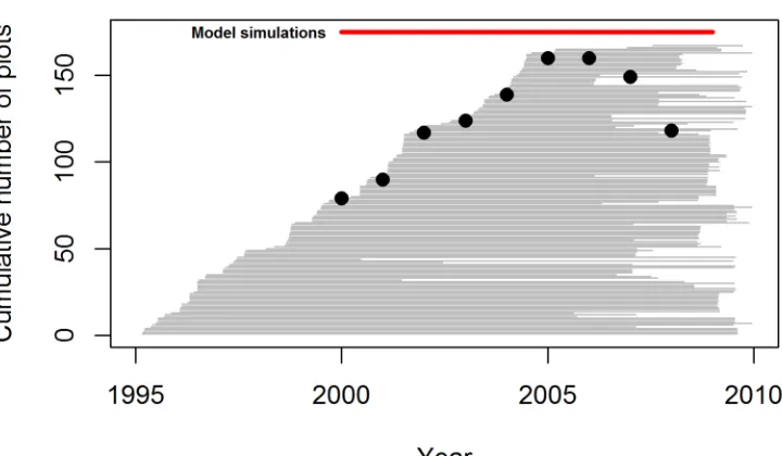
Figure S1. Cumulative number of plots monitored during 2000-8, and census periods covered by all
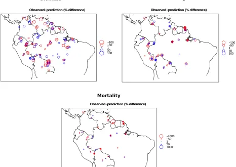
Figure S2. Semivariograms of variability in above ground biomass, above ground woody
productivity and stem-based mortality rates with distance (km) based on RAINFOR long-term plot
[image:15.595.123.483.191.609.2]Figure S3. Mean precipitation, maximum cumulative water deficit (MWD), temperature and short wave radiation for 2000-2008 from the
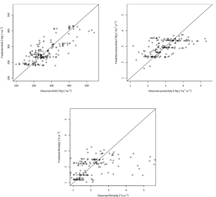
[image:16.842.135.646.157.512.2]Figure S4. Predicted values of above ground biomass, above ground woody productivity and stem-based mortality rates using a leave one out
Figure S9. Relationships between simulated mean WP and AGB from the 4 DGVMs, and precipitation and mean water deficit.
0 1 2 3 4
0 5 1 0 1 5 ORCHIDEE 0.46 r=
0 1 2 3 4
0 5 1 0 1 5 JULES 0.49 r=
0 1 2 3 4
0 5 1 0 1 5 INLAND 0.77 r=
0 1 2 3 4
0 5 1 0 1 5 LPJmL 0.82 r=
−800 −400 0
0 5 1 0 1 5 ORCHIDEE 0.51 r=
−800 −400 0
0 5 1 0 1 5 JULES 0.5 r=
−800 −400 0
0 5 1 0 1 5 INLAND 0.74 r=
−800 −400 0
0 5 1 0 1 5 LPJmL 0.92 r=
0 1 2 3 4
0 5 0 1 5 0 2 5 0 3 5 0 ORCHIDEE 0.66 r=
0 1 2 3 4
0 5 0 1 5 0 2 5 0 3 5 0 JULES 0.43 r=
0 1 2 3 4
0 5 0 1 5 0 2 5 0 3 5 0 INLAND 0.74 r=
0 1 2 3 4
0 5 0 1 5 0 2 5 0 3 5 0 LPJmL 0.8 r=
−800 −400 0
0 5 0 1 5 0 2 5 0 3 5 0 ORCHIDEE 0.74 r=
−800 −400 0
0 5 0 1 5 0 2 5 0 3 5 0 JULES 0.43 r=
−800 −400 0
0 5 0 1 5 0 2 5 0 3 5 0 INLAND 0.72 r=
−800 −400 0
0 5 0 1 5 0 2 5 0 3 5 0 LPJmL 0.81 r= N P P w o o d ( M g C h a -1y r -1) N P P w o o d ( M g C h a -1y r -1)
Precip(myr-1) Precip(myr-1)
N P P w o o d ( M g C h a -1y r -1) N P P w o o d ( M g C h a -1y r -1)
MWD (mm) MWD (mm)
A G B w o o d ( M g C h a -1) A G B w o o d ( M g C h a -1)
Precip(myr-1)
Precip(myr-1)
A G B w o o d ( M g C h a -1) A G B w o o d ( M g C h a -1)
Figure S10. Relationships between simulated mean WP and AGB from the 4 DGVMs, and short wave radiation and temperature.
160 200 240
0 5 1 0 1 5 ORCHIDEE −0.08 r=
160 200 240
0 5 1 0 1 5 JULES −0.08 r=
160 200 240
0 5 1 0 1 5 INLAND −0.27 r=
160 200 240
0 5 1 0 1 5 LPJmL −0.47 r=
5 10 15 20 25
0 5 1 0 1 5 ORCHIDEE 0.58 r=
5 10 15 20 25
0 5 1 0 1 5 JULES 0.09 r=
5 10 15 20 25
0 5 1 0 1 5 INLAND 0.59 r=
5 10 15 20 25
0 5 1 0 1 5 LPJmL 0.4 r=
160 200 240
0 5 0 1 5 0 2 5 0 3 5 0 ORCHIDEE −0.33 r=
160 200 240
0 5 0 1 5 0 2 5 0 3 5 0 JULES −0.14 r=
160 200 240
0 5 0 1 5 0 2 5 0 3 5 0 INLAND −0.27 r=
160 200 240
0 5 0 1 5 0 2 5 0 3 5 0 LPJmL −0.56 r=
5 10 15 20 25
0 5 0 1 5 0 2 5 0 3 5 0 ORCHIDEE 0.45 r=
5 10 15 20 25
0 5 0 1 5 0 2 5 0 3 5 0 JULES 0.19 r=
5 10 15 20 25
0 5 0 1 5 0 2 5 0 3 5 0 INLAND 0.59 r=
5 10 15 20 25
0 5 0 1 5 0 2 5 0 3 5 0 LPJmL 0.36 r= N P P w o o d ( M g C h a -1y r -1) N P P w o o d ( M g C h a -1y r -1)
SWrad(Wm-2)
SWrad(Wm-2)
N P P w o o d ( M g C h a -1y r -1) N P P w o o d ( M g C h a -1y r -1)
Temp(C) Temp(C)
A G B w o o d ( M g C h a -1) A G B w o o d ( M g C h a -1)
SWrad(Wm-2)
SWrad(Wm-2)
A G B w o o d ( M g C h a -1) A G B w o o d ( M g C h a -1)