This is a repository copy of
Predictive control design on an embedded robust
output-feedback compensator for wind turbine blade-pitch preview control
.
White Rose Research Online URL for this paper:
http://eprints.whiterose.ac.uk/101834/
Version: Accepted Version
Proceedings Paper:
Lio, W.H. orcid.org/0000-0002-3946-8431, Rossiter, J.A. and Jones, B.L. (2016) Predictive
control design on an embedded robust output-feedback compensator for wind turbine
blade-pitch preview control. In: European Control Conference 2016. European Control
Conference 2016, 29 Jun - 01 Jul 2016 . ISBN 978-1-5090-2590-9
[email protected] https://eprints.whiterose.ac.uk/
Reuse
Unless indicated otherwise, fulltext items are protected by copyright with all rights reserved. The copyright exception in section 29 of the Copyright, Designs and Patents Act 1988 allows the making of a single copy solely for the purpose of non-commercial research or private study within the limits of fair dealing. The publisher or other rights-holder may allow further reproduction and re-use of this version - refer to the White Rose Research Online record for this item. Where records identify the publisher as the copyright holder, users can verify any specific terms of use on the publisher’s website.
Takedown
If you consider content in White Rose Research Online to be in breach of UK law, please notify us by
Predictive control design on an embedded robust output-feedback
compensator for wind turbine blade-pitch preview control
Wai Hou Lio, J.A. Rossiter and Bryn Ll. Jones
Abstract— The use of upstream wind measurements has motivated the development of blade-pitch preview controllers to improve rotor speed tracking and structural load reduction beyond that achievable via conventional feedback design. Such preview controllers, typically based upon model predictive control (MPC) for its constraint handling properties, alter the closed-loop dynamics of the existing blade-pitch feedback control system. This can result in the robustness properties of the original closed-loop system being no longer preserved. As a consequence, the aim of this work is to formulate a MPC layer on top of a given output-feedback controller, with a view to retaining the closed-loop robustness and frequency-domain performance of the latter. The separate nature of the proposed controller structure enables clear and transparent qualifications of the benefits gained by using preview and predictive control. This is illustrated by results obtained from closed-loop simulations upon a high-fidelity turbine, showing the performance comparison between a nominal feedback compensator and the proposed MPC-based preview controller.
I. INTRODUCTION
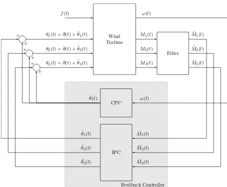
The rotor and structural components of large wind turbines are subjected to unsteady and intermittent aerodynamic loads from the wind. Such unsteady loads cause the rotor speed and power generation to exceed the design specification and also lead to fatigue damage to key turbine structural com-ponents, resulting in a reduction of the operational lifetime. Most wind turbines are equipped with blade-pitch controllers for achieving turbine speed regulation in above-rated wind conditions. An increasing number of large wind turbines are beginning to exploit the adjustment of blade pitch angle to attenuate unbalanced loads on the rotor. These two strategies are commonly known as: (i) collective pitch control (CPC), whose role is to regulate rotor speed by adjusting the pitch angle of each blade by the same amount, and (ii) individual pitch control (IPC), which provides an additional pitch angle demand signal, typically in response to measurement of flap-wise blade bending moments, to attenuate the effect of unsteady loads on the rotor (e.g. [1], [2]).
In recent years, a growing body of research has emerged, seeking to utilise real-time measurement of wind conditions from remote sensing devices for feed-forward control design. Some earlier results studied the use of preview control design for CPC (e.g. [3]) and suggested significant performance improvement over feedback-only designs; the first field test on feed-forward CPC design was reported by [4]. Lately, [5] investigated IPC design with advance wind knowledge and
All authors are with Department of Automatic Control and Sys-tems Engineering, The University of Sheffield, Sheffield, S1 3JD, U.K.
{w.h.lio|j.a.rossiter|b.l.jones}@sheffield.ac.uk
concluded that the feed-forward IPC design should include a careful consideration of the pitch actuator activity. As a consequence, several authors (e.g. [6]–[8]), employed model predictive control (MPC) in a preview IPC design owing to its ability to handle constraints and feed-forward information, and their results demonstrated the efficacy of a preview MPC design in the flap-wise blade load reduction.
The majority of wind turbine preview MPC studies can be divided into two categories. The first branch is to formulate the blade-pitch control problem as one single MPC formu-lation where the resultant controller handles both feedback and feed-forward measurements (e.g. [7]), whilst the second branch is to construct the MPC layer based on a known state-feedback controller (e.g. [6]). The shortcomings of both methods are that the robustness and closed-loop frequency-domain properties are usually not well considered in a stan-dard MPC design. The loads on turbine blades predominately exist at the harmonics of the blade rotational frequency, thus, it is not straightforward to design robust closed-loop feedback controllers in the time-domain. Furthermore, it is often assumed that the existing controllers use full state-feedback, despite the fact that output-feedback controllers are prevalent in industry.
This work therefore aims to bridge this gap by formulating a MPC layer based on a known robust output-feedback controller, where the MPC layer handles constraints and upcoming wind measurements. A further key focus of this paper stems from existing research often overlooking the conditions that separate the original closed-loop dynamics from the additional control layer design. If the given closed-loop dynamics are changed by the extra layer design, as a consequence, the benefits of utilising real-time measurement of the upstream wind become less transparent. The separate nature of the MPC layer is important from an industry perspective, since it can be implemented without replacing the existing feedback controller. Also, it provides a clear framework to quantify the benefits of feed-forward and predictive control over a baseline feedback strategy.
Wind Turbine
CPC
IPC
Filter
θ1(t) = ¯θ(t) + ˜θ1(t)
θ2(t) = ¯θ(t) + ˜θ2(t)
θ3(t) = ¯θ(t) + ˜θ3(t)
+ +
+ +
+ +
M1(t) M˜1(t)
˜
M1(t)
M2(t) M˜2(t)
˜
M2(t)
M3(t) M˜3(t)
˜
M3(t)
˜
θ1(t)
˜
θ2(t)
˜
θ3(t)
ω(t)
ω(t) ¯
θ(t)
f(t)
[image:3.612.62.289.55.242.2]Feedback Controller
Fig. 1. System architecture of a wind turbine blade-pitch control system, combining of collective pitch control (CPC) and individual pitch control (IPC). The CPC regulates rotor speed while the IPC attenuates perturbations in the flap-wise root bending moments on each blade. Additional inputs to the turbine, such as wind loading and generator torque, are accounted for in the termf(t)
feedback controller. Conclusions are in Section V.
II. WIND TURBINE MODELLING AND NOMINAL ROBUST FEEDBACK COMPENSATOR
This section presents background on the wind turbine model and disturbances. In addition, the details of the embedded nominal robust feedback controller are discussed.
A. Wind turbine modelling
A typical wind turbine blade pitch control system archi-tecture for above-rated conditions is depicted in Figure 1. The CPC regulates the rotor speed ω(t) by adjusting the collective pitch angle signal whilst the IPC attenuates loads by providing additional pitch signals on top of the collective pitch angle in response to flap-wise blade root bending moment signals. To isolate the action of the IPC from the CPC (e.g. [1], [9]–[11]), it is convenient to define the pitch angles and blade moments as follows:
"θ
1(t) θ2(t) θ3(t)
#
:=
¯
θ(t) + ˜θ1(t)
¯
θ(t) + ˜θ2(t)
¯
θ(t) + ˜θ3(t)
, "M
1(t) M2(t) M3(t)
#
:=
¯
M(t) + ˜M1(t)
¯
M(t) + ˜M2(t)
¯
M(t) + ˜M3(t)
(1)
For simplicity, it is assumed that there is no coupling between the CPC and IPC loops from the tower dynamics. The relationship between collective pitch inputθ¯(t)and rotor speed output ω(t) can be modelled by a transfer function Gωθ(s)obtained by linearising the turbine dynamics around the operating wind condition of 18 ms−1, chosen because
this value is close to the centre of the range of wind speeds covering the above-rated wind condition. Similarly, the re-lationship mapping the perturbations in flap-wise blade root bending moment M˜1,2,3 to additional pitch angle θ˜1,2,3 of
each blade can be modelled by a transfer functionGM θ(s). These transfer functions are as follows:
Gωθ(s) :=Ga(s)Gr(s), (2a) GM θ(s) :=Ga(s)Gb(s)Gbp(s), (2b)
where Gr(s), Gb(s) and Ga(s) describe the dynamics of
rotor, blade and actuator, respectively, whilst Gbp(s) is a
band-pass filter that is included in order to remove the low and high frequency contents of the blade root bending measurement signals, obtained from strain-gauge sensors. These transfer functions are defined as follows:
Gr(s) := ∂ω
∂θ
1
τrs+ 1
, (3a)
Gb(s) := ∂Mflap
∂θ
(2πfb)2
s2+ 4πfbDbs+ (2πfb)2, (3b)
Ga(s) :=
1
τ s+ 1, (3c)
Gbp(s) :=
2πfh s2+ 2π(f
h+fl)s+ 4π2fhfl
, (3d)
where ∂ω∂θ and τr denote the the variation in rotor speed
to pitch angle and time constant of the rotor dynamics, whilst ∂Mflap
∂θ ,Dbandfbrepresent change in blade bending moment to pitch angle, blade damping ratio and natural frequency of first blade mode, respectively. The time constant of the pitch actuator is τ whilst fh and fl denote the
upper and lower cut-off frequencies of the band-pass filter, respectively. Values are listed in Table II.
B. Disturbance modelling
The rotor and blade are subjected to a temporally varying and spatially distributed wind field. Given the feasibility of estimating the wind-field from a few point measurements taken upstream of the turbine (e.g. [12] ), this work assumes the full approaching wind field is known a priori. The disturbance trajectories of rotor speedωdand flap-wise blade bending moment M˜di, for i ∈ {1,2,3}, caused by the approaching wind, are defined as follows:
ωd(k) :=X
l,φ ∂ω
∂v(¯v, l)v(l, φ) (4)
˜
Mdi(k) :=X
l,φ ∂Mflap
∂v (¯v, l)v(l, φ), i= 1,2,3 (5)
wherev(l, φ)denote the stream-wise wind speed measure-ments where l and φ represent the radial and angular co-ordinates across the rotor disk whilstv¯denote the averaged wind speed of the measurements. Noted that span-wise and vertical wind speed is assumed negligible because the turbine blades spin fast in span-wise and vertical directions. The variations in rotor speed and blade bending moment with respect to the wind are denoted as ∂ωd
∂v and ∂Md
∂v . The rotor speed response ω to wind-induced disturbance ωd is modelled as a first-order transfer function Gωωd(s), whilst the response of flap-wise blade root bending momentM˜i to wind-induced disturbanceM˜di, fori∈ {1,2,3}, is modelled asGM Md(s):
Gωωd(s) := 1
τrs+ 1
, (6a)
GM Md(s) := (2πfb)
2
s2+ 4πf
bDbs+ (2πfb)2
Combining (2) and (6), the overall transfer function models G(s)andGd(s)can be represented as follows:
ω(s) ˜
M1(s)
˜
M2(s)
˜
M3(s)
=
Gωθ(s) 0 0 0
0 GM θ(s) 0 0
0 0 GM θ(s) 0
0 0 0 GM θ(s)
| {z }
G(s)
¯
θ(s) ˜
θ1(s)
˜
θ2(s)
˜
θ3(s)
+
Gωωd(s) 0 0 0
0 GM Md(s) 0 0
0 0 GM Md(s) 0
0 0 0 GM Md(s)
| {z }
Gd(s)
ωd(s) ˜
Md1(s) ˜
Md2(s)
˜
Md3(s)
(7)
Equivalently, a discrete-time state-space model representa-tion can be constructed as follows:
xpk+1=Apxpk+Bpuk+B p
ddk, (8a) yk=Cpx
p
k, (8b)
uk = [¯θk,θ˜1k,θ˜2k,θ˜3k]
T
, (8c)
yk = [ωk,M˜1k,M˜2k,M˜3k]
T
, (8d)
dk = [ωdk,M˜d1k,
˜ Md2k,
˜ Md3k]
T
, (8e) where superscript pdenotes plant.
C. Nominal embedded robust feedback controller
The chosen robust feedback controller K(s), consisting of the CPCKθω(s)and the IPCKθM(s), employed in this work is defined as follows:
¯
θ(s) ˜
θ1(s)
˜
θ2(s)
˜
θ3(s)
=
Kθω(s) 0 0 0
0 KθM(s) 0 0
0 0 KθM(s) 0
0 0 0 KθM(s)
| {z }
K(s)
ω(s) ˜
M1(s)
˜
M2(s)
˜
M3(s)
(9)
where Kθω(s) and KθM(s) obtained from [11], are pre-sented in Appendix I. It is assumed no dynamic coupling exists between the fixed and rotating turbine structures. The simulation results in [11] showed that a controller of the form (9) could be designed to be insensitive to such coupling by shaping the open-loop frequency response to have low gain at the tower frequency. Similar to the plant model, the nominal feedback controller (9) in a discrete time state-space realisation is:
xκk+1=A
κ xκk−B
κ
yk, (10a)
uk =Cκxκk−D κ
yk, (10b)
where the vectorxκrepresents the state of the controller and the superscriptκdenotes controller.
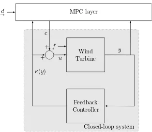
III. FORMULATION OF THEMPCLAYER
The architecture combining the proposed MPC layer and the nominal feedback controller is shown in Figure 2, where the shaded area depicts the existing closed-loop system. The closed-loop system dynamics in a state-augmented form can
Wind Turbine Feedback Controller + + MPC layer y u
κ(y) c
f d
→
[image:4.612.357.514.55.191.2]Closed-loop system
Fig. 2. Concept of model predictive control layer on top of a known feedback controller.
be derived from the discrete-time state-space wind turbine model (8) and the feedback controller (10):
xpk+1 xκ k+1 uk =
Ap 0 Bp
−BκCp Aκ 0
0 0 I
| {z }
A
xpk xκ k uk−1
| {z }
xk + Bp 0 I
| {z }
B
∆uk+
Bdp
0 0
| {z }
Bd dk
(11a)
∆uk=Kxk=
h
−DκCp Cκ −I
i
xk (11b)
yk=Cxk=
h
Cp 0 0ixk (11c)
Note that an incremental input ∆uk is employed in the state-augmented closed-loop system model (11a) as the input variable because of the simplicity of formulation of blade pitch rate and angle constraints.
A. Augmentation of input perturbations into the underlying feedback control law
The MPC formulation in this work adopts a closed-loop paradigm [13] where the degrees-of-freedom (d.o.f)ck can be set up around the stabilising feedback control law (11b) ∆uk = Kxk such that the input can be parametrised as ∆uk = Kxk +ck with the premise that the perturbation ck 6= 0 if and only if constraints are active or feed-forward knowledge is available. Such a feature is particularly useful in formulating a MPC layer on top of an embedded closed-loop controller. The closed-closed-loop paradigm employed in this work uses a dual-mode approach and these two modes of predictions are the transient mode and the terminal mode. In transient mode, a sequence of input d.o.f.s, denoted as
c
→k= [c0|k, c1|k, ..., cnc−1|k] T
, is optimised over the control horizon nc in respect to handling of constraints and feed-forward information, whilst in the terminal mode, the closed-loop dynamics are governed by the pre-determined control law, which is the embedded robust feedback pitch controller in this case. Considering (11a), the predictions of input and state at sample timekcan be described as follows:
∆ui|k=
(
Kxi|k+ci|k, ∀i < nc,
Kxi|k, ∀i≥nc,
(12a)
xi+1|k=
(
Φxi|k+Bci|k+Bddi|k, ∀i < nc,
Φxi|k+Bddi|k, ∀i≥nc,
whereΦ =A+BK. Noted thatx0|k=xk. The predictions of disturbance measurement d
→k = [d0|k, d1|k, ..., dna−1|k] T
is defined as follows:
di|k =
(
dk+i, ∀i < na 0, ∀i≥na.
(12c)
It is assumed that beyond the preview horizon na, the upcoming disturbance measurement becomes zero. Subse-quently, it is more convenient to represent the dual-mode predictions in one autonomous model such that the model consists of state predictions (12b), input prediction se-quence (12a) and advance disturbance measurement (12c). The autonomous model with the augmented state zi|k is defined as follows:
zi+1|k = Ψzi|k (13a) where the initial augmented state z0|k = [xT0|k, c→
T k, d→
T k]
T
andΨis defined as:
Ψ =
Φ BE BdE 0 Mc 0 0 0 Md
, (13b)
E c
→k=c0|k, E d→k=d0|k, (13c) Mcc
→= [c
T
1|k, ..., c T
nc−1|k,0] T
, (13d)
Mdd
→= [d
T
1|k, ..., d T
na−1|k,0] T
. (13e)
Consequently, the prediction of state and input (employed in the cost function) can be expressed in terms of the autonomous model (13a) as follows:
xi|k =
I 0 0
| {z }
Γx
zi|k, ∀i≥0, (14a)
∆ui|k =
K E 0
| {z }
Γu
zi|k, ∀i≥0. (14b)
B. Formulation of the cost function
The input perturbation sequence c
→k is computed by solv-ing a constrained minimisation of the predicted cost where the predicted cost function quantifying the balance between performance and input effort is defined as follows:
J :=
∞
X
i=0
h
xT
i|kQxi|k+ ∆uTi|kR∆ui|k+ 2xTi|kN∆ui|k
i
(15) whereQ,RandNdenote the weighting matrices that specify the penalties on state and input in the cost. For practical reasons, the infinite-horizon cost function (15) needs to be expressed in a finite-horizon form such that it can be solved on-line rapidly by quadratic programming. By expressing the prediction of the deviation variables of state (14a) and input (14b) in terms of the autonomous model, the cost function (15) can be simplified as follows:
J :=z0T|k
∞
X
i=0
ΨiTΓTxQΓx+ ΓuTRΓu+ 2ΓTxNΓu
| {z }
W
Ψi
| {z }
S
z0|k
(16)
Consequently, the cost function (16) can be further simpli-fied, using the Lyapunov equationΨTSΨ =S−W
, as:
J:=
x0|k c →k
d →k
T
Sx Sxc Sxd SxcT Sc Scd ST
xd S T cd Sd
| {z }
S
x0|k c →k
d →k
| {z }
z0|k
(17)
C. Constraint formation in terms of input perturbations
The physical limits on pitch actuator rate and angle are considered as hard constraints in this work. The limits on pitch rate are±8 degrees per second, whilst the pitch angle is bounded between 0 degree and 90 degrees:
∆u≤∆ui|k ≤∆¯u, ∀i≥0, (18a) u≤ui|k≤u,¯ ∀i≥0. (18b) These inequalities can be written in terms of the autonomous model (13a), withzi|k = Ψiz0|k, as follows:
HΨiz0|k≤f, ∀i≥0. (18c) where Hzi|k = [ui|k,−ui|k,∆ui|k,−∆ui|k]T and f = [¯u, u,∆¯u,∆u]T
. It is noted that to ensure no constraint vio-lations, possible violations must be checked over an infinite prediction horizon. Nevertheless, there exists a sufficiently large horizon where any additional linear equalities become redundant [14]. Consequently, for a practical approach, this study formulates the inequalities by checking the constraints over twice the control horizon and the inequalities can be described by a set of suitable matrices (M,N,V and b) as follows:
Mxk+N→c
k+V→dk≤b. (19) To sum up the discussion so far, the optimal input pertur-bation sequence c
→k from the MPC layer can be computed by solving a minimisation of the predicted cost function (17) subject to constraints (19). This is summarised in Algo-rithm 1:
Algorithm 1: At each sampling instant perform the opti-misation below. The first block element of the perturbation
c
→k is applied within the embedded control law (12a): min
c →k
c →
T
kSc→ck+ 2→c
T kS
T
xcx0|k+ 2→cTkScdd
→k (20a) s.t. Mxk+Nc
→k+V→dk≤b (20b)
D. Key result - Conditions for separating the original closed-loop dynamics from the additional layer design
The unconstrained optimal input sequence can be obtained by solving the minimisation of the cost (17) as follows:
c
→k =−Sc
−1
SxcTx0|k−Sc−1Scd→dk (21) Close inspection of (21) suggests that, to retain the closed-loop robust properties, the perturbation sequence c
→k must be independent of the statex0|k (i.e.SxcT = 0 in the cost).
Theorem 1: The input perturbation sequence c
true only if the cost function in Algorithm 1 embeds some knowledge of the nominal output-feedback control law (10) such that the weightsQ,R,N andSxsatisfy the following conditions:
ΦT
SxΦ−Sx+Q+KTRK = 0, (22a) BTSxΦ +RK+NT = 0. (22b)
Proof: This is straightforward to demonstrate by inves-tigating the cost function (17) and the Lyapunov equation ΨTSΨ =S−W
.
Corollary 1: This theorem is significant because it demonstrates that the extra MPC layer will not impact on the underlying robust closed-loop properties unless constraints are predicted to be active. Consequently, in normal operation, the properties of the underlying robust law are retained.
Nevertheless, a key point in the observation above is consistency between the performance index in Algorithm 1 and the underlying robust control law of (11b). Since the underlying controllers (10) employed in this work were designed using frequency-shaped technique, the weights that satisfy the conditions (22) can be determined by solving a linear matrix inequality (LMI) problem [15].
IV. NUMERICAL RESULTS AND DISCUSSIONS This section demonstrates the efficacy and performance benefits of the use of the combined MPC/robust control structure by performing closed-loop simulations on a high-fidelity wind turbine model.
A. Simulation environment and settings
The turbine model employed in this study is the NREL 5MW turbine [16] based on the FAST code [17]. This model is of much greater complexity than the model (7) employed for control design and includes flap-wise and edge-wise blade modes, in addition to tower and drive train dynamics. The wind field generated by the TurbSim code [18] numerically simulates the time series of a three-dimensional wind vectors at points in a two-dimensional vertical rectangular grid such that the series of grids march towards the rotor specified by the mean wind speed and under the assumption of Taylor’s frozen turbulence hypothesis. The upcoming stream-wise wind speed measurements on a 17-by-17 grid across the rotor plane were obtained from the TurbSim code. Nevertheless, the feed-forward inputs based on such turbulent wind mea-surements were aggressive and ineffective, thus, to remove the spatial turbulences that are less sensitive to turbine loads, the measurements of the turbulent wind fieldvm(yr, zr)can
be reconstructed into a simplified wind fieldv(yr, zr):
v(yr, zr) = ¯v+δhyr+δvzr (23)
whereyr andzr are the horizontal and vertical co-ordinates
across the rotor plane. The averaged wind speed, horizontal and vertical shear components are denoted as ¯v, δh and δv, respectively, and these values were obtained on-line by performing least squares over the wind speed measurements vm(yr, zr) [19]. Subsequently, these simplified wind speed
measurement would be employed in (6) to estimate the disturbance trajectories.
B. Tuning of the MPC layer
The predictive controller should anticipate the upcoming wind far enough ahead to allow beneficial feed-forward compensation; it was found that na = 15 samples was a reasonable choice in this simulation setting. The operating frequency of the MPC controller was 5 Hz which gives a good compromise between performance and computational burden; hence the preview horizon is 3 seconds ahead. It is clear that a similar idea also holds true for the control horizonnc. The control horizon must be at least as large as the preview horizon, for the reason that the MPC controller can then plan effective control sequences to compensate for the wind disturbance.
C. Simulation results
The closed-loop simulation was performed under a tur-bulent wind field characterised by the mean speed of 13 ms−1 and turbulence intensity of 14%. Three controllers
were investigated: (i) the baseline robust feedback controller based on the control law (10) denoted as (FB); (ii) (FB/FF) represents the unconstrained additional layer on top of the baseline feedback compensator where the unconstrained input perturbation (21) is simply added to the feedback control law and (iii) the constraint-aware additional layer augmented with the embedded baseline feedback controller, where the input perturbation is computed on-line by solving Algorithm 1, denoted as (FB/MPC).
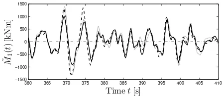
Figure 3 shows the sample time history excerpted from a 20-minute simulation result. Figure 3(a) illustrates the time history for the pitch angle of blade 1 where the controllers reached the pitch angle constraints and behaved differently. Consequently, in Figure 3(b), the rotor speed deviation for FB/MPC was slightly better than FB/FF. More importantly, Figure 3(c) shows significant reductions in flap-wise blade bending moment achieved by FB/MPC compared to FB/FF. The results from the full 20 minute simulation are sum-marised in Table I. As shown in Table I, it is not surprising that FB/FF and FB/MPC achieved lower standard deviations on rotor speed and blade load rejections compared to FB since they used of approaching wind measurements. Further-more, the results showed that the constraint-aware controller FB/MPC also outperformed FB/FF slightly. The difference is not significant because violations of pitch actuator constraints were infrequent. It is surmised that better improvement could be achieved by FB/MPC if soft-constraints on rotor speed and blade loads were also included.
V. CONCLUSION
360 365 370 375 380 385 390 395 400 405 410 0
2 4 6 8 10 12
θ1
(
t
)
[d
eg
]
Timet[s] FB
FB/FF FB/MPC
(a) Time history of the pitch angle of blade 1. Dash-dot lines represent the pitch angle constraint at 0 degree.
360 365 370 375 380 385 390 395 400 405 410 −1
−0.8 −0.6 −0.4 −0.2 0 0.2 0.4 0.6 0.8 1
∆
ω
(
t
)
[r
p
m
]
Timet[s]
(b) Time history of the rotor speed deviation. Dash-dot line represents the targeted rotor speed.
360 365 370 375 380 385 390 395 400 405 410
−1500 −1000 −500 0 500 1000 1500
˜M
1
(
t
)
[k
Nm
]
Timet[s]
[image:7.612.65.289.311.408.2](c) Time history of the flap-wise blade root bending moment of blade 1. Dash-dot line represents the targeted blade loads.
Fig. 3. Simulation results upon the NREL 5MW turbine, showing the performance of the various controllers studied in this paper.
TABLE I
CONTROLLER PERFORMANCE COMPARISONS
Description FB (Baseline) FB/FF FB/MPC std(ω)(rpm) 0.32 (100%) 0.27 (84%) 0.27 (84%) std(M˜1) (kNm) 629 (100%) 589 (94%) 581 (92%)
std(θ˙1) (deg s−1) 1.60 (100%) 1.56(98%) 1.56 (98%)
Note that std denotes the standard deviation. The percentage in bracket represents the relative difference to the baseline controller.
by the proposed MPC-based preview controller. Future work will include constraints on rotor speed and blade loads.
APPENDIXI
The model parameters for (7) are shown in Table II and the closed-loop robust controllers are described as follows:
Kθω(s) = 10.74s+ 3.845
3.142s (24a)
KθM(s) = 104× 2.3s
4+ 6.1s3+ 25.4s2+ 18.1s+ 39
(s4+ 0.20s3+ 8.06s2+ 0.46s+ 10.38) (24b)
TABLE II
MODEL PARAMETER OFG(s)(7)
Parameters Values Units Parameters Values Units
∂ω
∂θ −0.84rpm deg−1 ∂Mflap
∂θ −9.02×10⁵Nm deg−1
τr 4 s fb 0.70 Hz
Db 0.47 - τ 0.11 s
fh 0.80 Hz fl 0.014 Hz
REFERENCES
[1] K. Selvam, S. Kanev, J. W. van Wingerden, T. van Engelen, and M. Verhaegen, “Feedback-feedforward individual pitch control for wind turbine load reduction,” International Journal of Robust and
Nonlinear Control, vol. 19, no. 1, pp. 72–91, 2009.
[2] W. Leithead, V. Neilson, and S. Dominguez, “Alleviation of Unbal-anced Rotor Loads by Single Blade Controllers,” inEuropean Wind
Energy Conference & Exhibition, 2009.
[3] D. Schlipf, T. Fischer, and C. Carcangiu, “Load analysis of look-ahead collective pitch control using LIDAR,” inProc. of 10th German Wind
Energy Conference, 2010.
[4] D. Schlipf, P. Fleming, F. Haizmann, A. Scholbrock, M. Hofs¨aß, A. Wright, and P. W. Cheng, “Field Testing of Feedforward Collective Pitch Control on the CART2 Using a Nacelle-Based Lidar Scanner,”
inThe Science of Making Torque from Wind, 2012.
[5] J. Laks, L. Pao, and A. Wright, “Combined Feed-forward/Feedback Control of Wind Turbines to Reduce Blade Flap Bending Moments,”
inAIAA/ASME Wind Energy Symp., Orlando, FL, 2009.
[6] J. Laks, L. Pao, E. Simley, A. Wright, N. Kelley, and B. Jonkman, “Model Predictive Control Using Preview Measurements From LI-DAR,” in 49th AIAA. Reston, Virigina: American Institute of Aeronautics and Astronautics, 2011.
[7] M. D. Spencer, K. A. Stol, C. P. Unsworth, J. E. Cater, and S. E. Norris, “Model predictive control of a wind turbine using short-term wind field predictions,” Wind Energy, vol. 16, no. 3, pp. 417–434, 2013.
[8] Wai Hou Lio, J. Rossiter, and B. L. Jones, “A review on applications of model predictive control to wind turbines,” in 2014 UKACC
International Conference on Control (CONTROL). Loughborough,
U.K.: IEEE, 2014, pp. 673–678.
[9] E. A. Bossanyi, “Individual Blade Pitch Control for Load Reduction,”
Wind Energy, vol. 6, no. 2, pp. 119–128, 2003.
[10] Q. Lu, R. Bowyer, and B. Jones, “Analysis and design of Coleman transform-based individual pitch controllers for wind-turbine load reduction,”Wind Energy, vol. 18, no. 8, pp. 1451–1468, 2015. [11] W. H. Lio, B. L. Jones, Q. Lu, and J. Rossiter, “Fundamental
performance similarities between individual pitch control strategies for wind turbines,”International Journal of Control, 2015.
[12] P. Towers and B. L. Jones, “Real-time wind field reconstruction from LiDAR measurements using a dynamic wind model and state estimation,”Wind Energy, vol. 19, no. 1, pp. 133–150, 2016. [13] J. A. Rossiter,Model-Based Predictive Control: A Practical Approach.
CRC Press, 2003.
[14] E. Gilbert and K. Tan, “Linear systems with state and control con-straints: the theory and application of maximal output admissible sets,”
IEEE Transactions on Automatic Control, vol. 36, no. 9, pp. 1008–
1020, 1991.
[15] S. Boyd, L. El Ghaoui, E. Feron, and V. Balakrishnan,Linear Matrix
Inequalities in System and Control Theory. Society for Industrial and
Applied Mathematics, 1994.
[16] J. Jonkman, S. Butterfield, W. Musial, and G. Scott, “Definition of a 5-MW Reference Wind Turbine for Offshore System Development,” National Renewable Energy Laboratory (NREL), Golden, CO, Tech. Rep., 2009.
[17] J. Jonkman and M. Buhl Jr, “FAST User’s Guide,” National Renewable Energy Laboratory (NREL), Tech. Rep., 2005.
[18] B. Jonkman, “TurbSim User’s Guide,” National Renewable Energy Laboratory (NREL), Tech. Rep., 2009.