Linear rank-width and linear clique-width of trees

(1)

White Rose Research Online URL for this paper:

http://eprints.whiterose.ac.uk/101098/

Version: Accepted Version

Article:

Adler, I and Kante, MM (2015) Linear rank-width and linear clique-width of trees.

Theoretical Computer Science, 589. pp. 87-98. ISSN 0304-3975

https://doi.org/10.1016/j.tcs.2015.04.021

© 2015, Elsevier. Licensed under the Creative Commons

Attribution-NonCommercial-NoDerivatives 4.0 International

http://creativecommons.org/licenses/by-nc-nd/4.0/

[email protected] https://eprints.whiterose.ac.uk/ Reuse

Unless indicated otherwise, fulltext items are protected by copyright with all rights reserved. The copyright exception in section 29 of the Copyright, Designs and Patents Act 1988 allows the making of a single copy solely for the purpose of non-commercial research or private study within the limits of fair dealing. The publisher or other rights-holder may allow further reproduction and re-use of this version - refer to the White Rose Research Online record for this item. Where records identify the publisher as the copyright holder, users can verify any specific terms of use on the publisher’s website.

Takedown

If you consider content in White Rose Research Online to be in breach of UK law, please notify us by

(2)

Trees

⋆

Isolde Adler1⋆⋆ _{and Mamadou Moustapha Kant´e}2

1

Institut f¨ur Informatik, Goethe-Universit¨at, Frankfurt, Germany.

[email protected]

2

Clermont-Universit´e, Universit´e Blaise Pascal, LIMOS, CNRS, France.

[email protected]

Abstract We show that for every forest T the linear rank-width of T is

equal to the path-width ofT, and the linear clique-width of T equals the

path-width ofT plus two, provided thatT contains a path of length three.

It follows that both linear rank-width and linear clique-width of forests can be computed in linear time. Using our characterization of linear rank-width of forests, we determine the set of minimal excluded acyclic vertex-minors for the class of graphs of linear rank-width at mostk.

Keywords: Linear rank-width, linear clique-width, vertex-minors

1 Introduction

Rank-width [35] is a graph parameter introduced by Oum and Seymour with the goal of efficient approximation of the clique-width [11] of a graph. Linear rank-width can be seen as the linearized variant of rank-width, similar to path-width, which can be seen as the linearized variant of tree-width. While path-width is a well-studied notion, much less is yet known about linear rank-width. Any graph of

k-bounded path-width hask-bounded linear rank-width, but conversely the differ-ence is unbounded. For example, the class of all complete (bipartite) graphs has linear rank-width at most 1, but unbounded path-width.Linear clique-width, a lin-earized version of clique-width, was introduced independently by several authors when studying the computational complexity of clique-width [14,17,18,19,20,31]. Heggernes et al. [21,22,23] investigated computing linear clique-width on restricted graph classes.

Linear rank-width is equivalent to linear clique-width in the sense that any graph class has bounded linear clique-width if and only if it has bounded linear rank-width. Computing linear rank-width is NP-complete in general. In fact, it is proved in [14] that approximating linear clique-width is NP-hard and one can easily reduce the approximation of linear clique-width to the approximation of linear rank-width. Moreover, very little is known about efficient computation of linear rank-width on restricted graph classes. The only known results are for special types of graphs, such as for complete (bipartite) graphs, and linear clique-width is known to be polynomial time computable onthickened paths[23] andk-path powers [21]. Even for the very natural class of forests efficient computability was open. In contrast, many classes are known that allow efficient computation of path-width [5,6,7,13,15,29,32,37].

In this paper, we provide the first non-trivial graph class on which linear rank-width can be computed in polynomial (even linear) time. We prove

Theorem 1 Linear rank-width and linear clique-width of forests can be computed in linear time.

⋆

A preliminary version of this paper appeared in [2].

⋆⋆

(3)

Since path-width of forests can be computed in linear time by [13], Theorem 1 is an immediate corollary of the following two theorems.

Theorem 2 The linear rank-width of any forest equals its path-width.

Theorem 3 LetT be a tree. IfT contains a path of length3, then the linear clique-width of T equals the path-width of T plus2. Otherwise, the linear clique-width of T equals the path-width ofT plus1.

The statements of Theorems 2 and Theorem 3 fail for graphs contaning cy-cles. While it was known that the class of all trees has unbounded linear rank-width (see [15] for a combinatorial proof) and unbounded path-rank-width, Theorem 2 is somewhat surprising, because it actually equates two structurally very differ-ent parameters: Path-width and linear rank-width are graph parameters based on linear orderings of the vertex set of the given graph. Intuitively, path-width seeks for an ordering that minimizes the maximum number of edges ‘crossing’ a cut of the ordering, while linear rank-width seeks to minimize the maximum rank of cer-tain matrices associated with the cuts of the ordering. Linear clique-width in turn seeks to minimize the number of colours that allow to construct the given graph by introducing (coloured) vertices one by one and adding edges based on the vertex colours.

It is known that the linear clique-width of any graph is bounded by its path-width plus 2 [14]. Since linear rank-path-width is bounded by linear clique-path-width, the same bound carries over to linear rank-width. We show that the linear rank-width of any graph is bounded by its path-width. This is not hard to prove, but it seems it was not written down yet. For forests we show that the converse holds, too.

The proof of Theorem 2 uses the characterization of path-width by the cops and invisible robber game [28]. Given an ordering of the vertices of a forestT witnessing the linear rank-width of T, we construct a winning strategy for the cops. Here it is not sufficient for the cops to search the vertices according to the given ordering, but a more involved strategy yields the result. Our proof method is constructive. It shows that, given ann-vertex tree and an ordering of its vertices witnessing its linear rank-width, we can transform the given ordering into a winning strategy for the cops (using the original ordering as ‘landnarks’), and hence into a path decomposition, in timeO(n2_·_log2₍_n_{)). For determining the linear clique-width of trees we take a}

different approach by giving a recursive characterization of the linear clique-width of trees. The ideas we introduce here might also be useful in future research on comparing width parameters.

It is known that tree-width and path-width do not increase when taking minors. Similarly, (linear) rank-width does not increase when taking vertex-minors [8,24]. For a graph G and a vertex xof G, thelocal complementation at x ofG consists in replacing the subgraph induced on the neighbors of xby its complement; and a graph H is a vertex-minor of G if H can be obtained from G by a sequence of local complementations and deletions of vertices. The set of minimal excluded vertex-minors is known to be finite for every class of graphs that is closed under vertex-minors and has bounded rank-width [34]. Moreover given k, the number of vertices of a minimal excluded vertex-minor for rank-width ≤ k is bounded by (6k+1 ₋₁₎_/_{5 [24], and hence one can theoretically compute the set of minimal}

exclude vertex-minors for rank-width≤kin time depending only onkby searching among all graphs of size at most (6k+1₋₁₎_/_{5 and keeping only the non-isomorphic}

(4)

excluded vertex-minors were established in [25]. Using Theorem 2, we determine the set of minimal excluded acyclic vertex-minors for linear rank-widthk. It turns out that they coincide with the minimal excluded minors for graphs of path-width at mostk that are acyclic [38].

Outline of the paper. Section 2 introduces the terminology, the notion of linear rank-width and the cops and invisible robber game. In Section 3 we prove that linear rank-width and path-width coincide on forests (Theorem 2), in Section 4 we prove Theorem 3 characterizing the linear clique-width of forests. In Section 5 we give the set of minimal excluded acyclic vertex-minors for the class of graphs of linear rank-width k, and we conclude with Section 6.

2 Preliminaries

For a set Awe denote the power set ofAby 2A_{. We let}_A_\_B_:=_{_x_∈_A_|_{x /}_∈_B_}

denote the difference of two sets A and B. For two sets A and B let A∆B := (A\B)∪(B\A) denote thesymmetric difference ofAandB. For an integern >0 we let [n] :={1, . . . , n}.

For sets R and C an (R, C)-matrix is a matrix where the rows are indexed by elements in R and columns are indexed by elements inC. (Since we are only interested in the rank of matrices, it suffices to consider matrices up to permutations of rows and columns.) For an (R, C)-matrixM, ifX ⊆RandY ⊆C, we letM[X, Y] be the submatrix ofM obtained by restrictingM to the rows and columns indexed by the elements belonging to X and Y, respectively. IfM is an (R, C)-matrix and when the context is clear we will identify the row indexed byx∈Rwithx(similarly for the column indexed byy∈C); hence we will say for instance that a subsetX of

Ris a basis for the rows ofM if the rows indexed byX form a basis for the rows of

M and similarly for other linear algebra terminologies involving rows or columns. In this paper, graphs are finite, simple and undirected, unless stated otherwise. Let G be a graph. We denote the vertex set of G by V(G) and the edge set by

E(G). We regard edges as two-element subsets ofV(G). For a vertexv∈V(G) we letNG(v) :={u∈V(G)| {v, u} ∈ E(G)} denote the set ofneighbors of v (in G).

The degree of v (in G) is deg_G(v) :=|NG(v)|. A partition ofV(G) into two sets X and Y (i. e. X∪˙ Y =V(G)) is called a cut in G, and we denote it by (X, Y). In a linear ordering x1, . . . , xn, each 1 ≤ i ≤ n−1 induces a cut (Xi, Yi) with Xi:={x1, . . . , xi} andYi :={xi+1, . . . , xn}.

A graph not containing a cycle is calledacyclic. Apath from uto v in a graph

G is a sequenceP :=u1, . . . , up of pairwise distinct vertices ofG, whereu0:=u1

and up :=v, such that {ui, ui+1} ∈E(G) for every 0≤i≤p−1, andpis called

thelengthofP. Aconnected graph is a graph where any two vertices are connected by a path. Aforest is an acyclic graph and atree is a connected forest. Aleaf of a tree is a vertex of degree one. Astar is a tree with at most one non-leaf vertex.

Thedistance between two verticesu, v ∈V(G) is the length of a shortest path from u to v. Arooted tree is a tree with a distinguished vertex r, called theroot. Theheight of a rooted tree is the maximal length of a path from the root to a leaf. For a rooted treeT with rootr and vertexv ∈V(T) we denote byTv _{the subtree}

ofT rooted atv and induced by those verticesu∈V(T) such that the path fromr

to ucontainsv. For a rooted treeT it is sometimes convenient to orient the edges ofT in the direction away from the root, thus obtaining anoriented tree.

Linear rank-width and path-width. Let G be a graph, and let AG be the

(5)

matrices.) Thelinear rank-widthofGis defined as lrw(G) := min

v1,...,vnlinear ordering ofV(G)

max

i∈[n−1]{rk(AG[Xi, Yi])}.

Apath decompositionofGis a pair (P, B), wherePis a path andB = (Bt)t∈V(P)

is a family of subsetsBt⊆V(G), satisfying

1. For every v∈V(G) there exists at∈V(P) such thatv∈Bt.

2. For every e∈E(G) there exists at∈V(P) such thate⊆Bt.

3. For every v∈V(G) the set{t∈V(P)|v∈Bt}is connected inP.

The width of a path decomposition (P, B) is defined as w(P, B) := max{|Bt| | t∈V(P)} −1. Thepath-width ofGis defined as

pw(G) := min{w(P, B)|(P, B) is a path decomposition ofG}.

Observation 4 The linear rank-width (or path-width) of a graph equals the maxi-mum of the linear rank-width (or path-width) of its connected components.

It is easy also to see thatcaterpillars, i.e. the graphs that contain a pathP such that every vertex has distance at most one to some vertex of P, have path-width

≤1. Indeed, the graphs of path-width at most 1 are precisely the disjoint unions of caterpillars. One can derive from [3] that graphs of linear rank-width at most 1 are exactly those that are locally equivalent to caterpillars (where two graphs G

and H are locally equivalent, ifH can be obtained from Gby a sequence of local complementations). Using a labelling scheme, Ganian [15] characterizes the graphs of linear rank-width at most 1 asthread graphs. It is worth noticing that the path-width of trees, as well as their linear rank-path-width, is not bounded. For example, the rooted binary treeThof heighthsatisfies pw(Th) =⌈h/2⌉[36], and a combinatorial

proof for the unboundedness of the linear rank-width of trees can be found in [15]. Before continuing let us first recall the following easy fact that was not written down anywhere.

Lemma 5 Any graphG satisfieslrw(G)≤pw(G).

Proof. Let (P, B) be a path decomposition of G of width pw(G). W. l. o. g. we may assume that (P, B) is such that any two distinct vertices t, t′ _∈_V₍_P_{) satisfy}

Bt6⊆Bt′. Assume that the vertices of P aret₁, . . . , t

m, appearing in this order on

the path. LetB′₍_t

1) :=B(t1), and for every 1< i≤mletB′(ti) :=B(ti)\B(ti−1).

Then the familyB′_{:= (}_B′₍_t

i))i∈[m] is a partition ofV(G) into non-empty sets. For

eachi∈[m] choose an ordering of the vertices inB′₍_t

i) and combine these orderings

to an ordering of V(G) that respects the path P. We claim that this ordering witnesses lrw(G)≤pw(G). At every cut in the ordering, the corresponding matrix has at most pw(G) non-zero rows. To see this, let (X, Y) be a cut in the ordering with X =B′₍_t

1)∪. . .∪B′(ti)∪X′ and Y =Y′∪B′(ti+2)∪. . .∪B′(tm), where B′₍_t

i+1) =X′∪˙ Y′ is a partition ofB′(ti+1) into two setsX′ and Y′ withY′ 6=∅.

By the definition of path decompositions, a vertexv∈B′₍_t

1)∪. . .∪B′(ti) is adjacent

to a vertex inY if and only ifv∈B(ti+1). LetX0be the set of such vertices. Now

only vertices inX0∪X′ can have neighbors inY. SinceX0∪X′⊆B(ti+1)\Y′ and

Y′₆₌_∅_{, it follows that the rank of the matrix at (}_{X, Y}_{) is at most pw(}_G_). _⊓_⊔

(6)

robber move on the vertices ofG. Some of the cops move to at mostkvertices and the robber stands on a vertex rnot occupied by the cops. At all times, the robber is invisible to the cops. Initially, no cops occupy vertices and the robber chooses a vertex to start playing. In each move, some of the cops fly in helicopters to at mostknew vertices. During the flight, the robber sees which position the cops are approaching and before they land she quickly tries to escape by running arbitrarily fast along paths of G to a vertex r′_{, not being allowed to run through a vertex} occupied by a cop. Hence, if X ⊆V(G) is the cops’ position, the robber stands on

r ∈ V(G)\X, and after the flight, the cops occupy the set Y ⊆V(G), then the robber can run to any vertex r′ _{within the connected component of} _G_\₍_X _∩_Y₎ containingr. The cops win if they land a cop via helicopter on the vertex occupied by the robber. The robber wins if she can always elude capture.

Aplay is a sequence of cop positionsX0, X1, X2, . . .withX0:=∅ and|Xi| ≤k

for alli. At each step of a play, we can describe the set ofclearedvertices as follows. At the position X0, the set of cleared vertices is A0 :=∅. After the cops’ move to

Xi (fori >0), the set of cleared vertices is

Ai:= (Ai−1∪Xi)\ {r∈V(G)|there is a path fromV(G)\Ai−1

torin G\(Xi−1∩Xi)}.

Winning strategies are defined in the usual way. The invisible cop-width of G, icw(G), is the minimum number of cops having a winning strategy onG.

A winning strategy for the cops ismonotone, if for any playX0, X1, X2, . . .played

according to the strategy, the sets A0, Ai, A2, . . . form a non-decreasing sequence

(with respect to ⊆). The monotone invisible cop-width of G, monicw(G), is the minimum number of cops having a monotone winning strategy on G.

Theorem 6 ([12]) Any graph Gsatisfiesmonicw(G) = pw(G) + 1.

3 Linear Rank-Width and Path-Width of Trees

This section is devoted to the proof of the converse of Lemma 5 for forests, showing that lrw(T) ≥ pw(T) holds for any forest T. By Observation 4 we can restrict ourselves to trees instead of forests. Our proof turns a linear ordering of V(T) witnessing lrw(T) into a winning strategy for k + 1 cops. Roughly, the idea is that k cops move from basis to basis along the matrices at the cuts, clearing the vertices along the ordering on their way. One additional cop is used to make the transitions. For an intuition, suppose the cops occupy a vertex setBcorresponding to a basis of the matrix AT[Xi, Yi] where (Xi, Yi) is the cut at index i. Now two

cases arise, depending on whether the next vertex vi+1 is spanned by the rows of

AT[Xi+1, Yi+1] corresponding toB or not. The following two lemmas deal with the

case thatvi+1 is spanned by the rows ofAT[Xi+1, Yi+1] (vi+1is ‘dependent’ on the

rows ofAT[Xi+1, Yi+1]). Lemma 7 highlights structural properties of the treeT in

this situation, and Lemma 8 shows the next cop move in this situation (clearing vertex vi+1). We start with a definition.

LetT be a tree and let (X, Y) be a cut inT. LetB ⊆X be a basis of the row space of AT[X, Y]. For x∈X\B withNT(x)∩Y 6=∅, i.e, the row vector of xin AT[X, Y] has a non-zero entry, let Bx ⊆B be the (unique) minimal subset of B

spanning x. Let Tx be the subgraph ofT with vertex setV(Tx) = X′∪˙Y′, where X′_:=_B

x∪ {x}andY′:=NT(Bx∪ {x})∩Y, and with edge setE(T′) :={{u, v} ∈ E(T)|u∈X′_{, v}_∈_Y′_}_{. We call} _T

x the B-basic tree ofx (at(X, Y)).With these

assumptions we have the following two lemmas.

(7)

1. Tx is a tree.

2. Each leaf zof Tx is a vertex inX′, and|NT(z)∩Y|=dTx(z) = 1.

3. The vertices inY′ _{have degree two in}_T

x. 4. |Y′_|₌_|_B

x|.

Proof. 1. Since T is a tree it suffices to show that Tx is connected. If not, Tx

has a component C that does not containx. Then C can be written as C =

B′ _∪₍_N

T(B′)∩Y) for some non-empty subset B′ ( Bx. Because X′ =Bx∪ {x} and Bx is the subset of B that spans the row of x in AT[X, Y], then

the rows of AT[X′, Y′] sum up to zero, and moreover since C is a component,

the rows of AT[X′, Y′] corresponding to B′ must already sum up to zero (to

see this, permute the rows and columns of AT[X′, Y′] in such a way, that the

resulting matrix is a block matrix with non-zero blocks only along the diagonal), a contradiction toB being a basis.

2. Since the rows ofAT[X′, Y′] sum up to zero, for every vertex y∈Y′, degTx(y)

is even, so y is not a leaf. Hence the leaves are in X′ _⊆_X_{. Since by definition} of Tx, all neighbors in Y of vertices in X′ belong to Tx, the leaves of Tx are

vertices inX with a unique neighbor inY.

3. By (1),Txis a tree. Choosexas a root and orient the edges ofTxaway from the

root. Recall that any vertex inY′_{has even degree in}_T

x. Towards a contradiction,

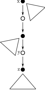
assume now that a vertex y∈Y′_{has degree}_≥_{4 (see Figure 1). Fix a successor}

z ofy inTx. All vertices of Y′ that lie in the subtreeTy\Tz have even degree

in Ty_\_Tz_{. But then the sum over all those rows of} _A

T[X′, Y′] that correspond

to vertices inTy_\_Tz _{is the zero vector, a contradiction to the fact that}_B _{is a}

basis. Hence every vertex in Y′ _{has degree 2 in}_T

x.

4. Follows from (1) and (3). ⊓⊔

x

y

[image:7.612.267.344.434.590.2]

z

Figure 1.The treeTx in the proof of Lemma 7. Triangles mean subtrees. Black vertices

are inX′_{, white vertices are in}_Y′ _{and all white vertices have degree 2.}

(8)

1. the vertices inX∪V(Tx)\ {x} are cleared, 2. all vertices in Y′ _{are occupied,}

3. exactly |Bx|cops occupy vertices of Tx.

Proof. Choose xas the root of Tx, and we letg :Bx→Y′ where for eachz ∈Bx

we letg(z) be the predecessor ofz in the orientation ofTx. From Lemma 7(3) and

Lemma 7(4) we know that g is a bijection. Roughly, the idea is that the cops occupying vertices of Bx move to Y′ according to the bijection g. This is done

bottom-up along Tx with the temporary employment of one additional cop.

By assumption, all vertices of Tx that lie in X′ \ {x} = Bx are cleared, and

for each vertex b∈Bx, eitherb is occupied by a cop, orNT(b)∩Y is occupied by

cops. The cops make a few moves such that for all b ∈ Bx, the set NT(b)∩Y is

occupied by cops. This is done as follows. For every leafbinTxthat is occupied by

a cop, we move the cop occupying b to the unique neighbor ofb in Y, i.e. to g(b). For this, we place the (k+ 1)st cop onbas well, and move the (one) cop frombto the neighbor in Y. By Lemma 7(2), the leaves ofTx have a unique neighbor inY.

Now, whenever all successors of a vertexb∈Bx⊆V(Tx) are occupied by cops, we

move the cop occupying b to g(b) (again with the temporary help of the (k+ 1)st cop). Proceeding like this from the leaves ofTxto the root, by Lemma 7(3), finally,

exactly the vertices inY′ _{are occupied by cops and the vertices in}_X_∪_V₍_T

x)\ {x}

are cleared. Part 3 follows from Lemma 7(4). This finishes the proof. ⊓⊔

Theorem 9 Any tree T satisfiespw(T)≤lrw(T). Moreover, givenT and a linear ordering of its vertex setV witnessinglrw(T), there is an algorithm of running time O(|V|2_·_log2₍_|_V_|₎₎_{that computes a path decomposition of}_T _{of width at most}_lrw(_T₎_.

Proof. If |V(T)| ≤1, then the theorem holds. Assume now that |V(T)| ≥ 2. Let

v1, . . . , vn be a linear ordering of V(T) witnessing k := lrw(T). For i ∈ [n] let Xi:={v1, . . . , vi}andYi:={vi+1, . . . , vn}.

We describe a strategy for k+ 1 cops. The strategy follows the linear ordering of V(T). For each new vertexvi that has to be cleared, we describe atransition –

a finite sequence of monotone cop moves to make sure thatvi is cleared. After the ith transition, the following invariants hold.

(I1) Every vertex inXi is cleared.

There is a basis Bi⊆Xi of the rows of AT[Xi, Yi] such that

(I2) eachb∈Bi satisfies:

bis occupied by a cop orNT(b)∩Yi is occupied by cops, and no vertex

in the setXi\Biis occupied by a cop.

(I3) The cops occupy exactly|Bi|vertices.

Let ℓ be the greatest index i ≤ k such that the rank of AT[Xi, Yi] is equal to i.

Then ℓ ≥1 because |V(T)| ≥ 2. The first ℓ transitions simply consist in placing cops on the vertices v1, . . . , vℓ, successively. Obviously, after each such transition,

the invariants hold.

Suppose we have completed theith transition, and we want to make the (i+1)st transition. Moving from AT[Xi, Yi] toAT[Xi+1, Yi+1], exactly one of the following

cases occurs.

(a) InAT[Xi+1, Yi+1], the new vertexvi+1 is in the span ofBi.

(9)

Observe that Bi can span the rows of AT[Xi+1, Yi+1], but may be linearly

de-pendent in AT[Xi+1, Yi+1]. If it is linearly dependent in AT[Xi+1, Yi+1], then the

size of a maximum linearly independent subset ofBi is|Bi| −1, because deleting a

column can only decrease the rank by one.

Claim 1:If the size of a maximum linearly independent subset ofBiinAT[Xi+1, Yi+1]

is|Bi| −1, then there exists a vertexvN ∈NT(vi+1)∩Bi such thatBi\ {vN}is a

maximum linearly independent subset ofBi in AT[Xi+1, Yi+1].

Proof of the Claim: If Bi is linearly dependent in AT[Xi+1, Yi+1] and linearly

independent inAT[Xi, Yi], there exists a row ofAT[Xi, Yi] corresponding to a vertex u∈Bi that is generated byBi\ {u}and that has a 1 at the column corresponding

tovi+1, and henceu∈NT(vi+1). ⊣

IfBiis linearly dependent inAT[Xi+1, Yi+1], we pickvN ∈NT(vi+1)∩Bias in

Claim 1 and we letB′

i:=Bi\vN. If Bi is linearly independent inAT[Xi+1, Yi+1],

we letB′

i :=Bi. Ifvi+1 is in the span of Bi, we letBi+1 :=Bi′. Otherwise, we let Bi+1:=Bi′∪ {vi+1}. Obviously,Bi+1is a basis of AT[Xi+1, Yi+1].

For each v spanned by Bi+1 let Tv denote theBi+1-basic tree of v at the cut

(Xi+1, Yi+1). The following follows from the fact thatT is a tree and the vertexvN

is adjacent tovi+1.

Claim 2:AssumingBiis linearly dependent inAT[Xi+1, Yi+1], letvN ∈NT(vi+1)∩

Bi be as in Claim 1.

(i) TheBi+1-basic tree ofvN does not containvi+1.

(ii) If moreovervi+1is spanned byBiinAT[Xi+1, Yi+1], thenV(Tvi+1)∩V(TvN) =∅

and there is no edge other than{vN, vi+1}between a vertex ofTvi+1and a vertex

ofTvN. ⊣

We distinguish two cases, depending on whether a cop occupiesvi+1.

Case 1.After theith transition, vi+1 is not occupied by a cop.

Then by the inductive invariant (I1), the set NT(vi+1)∩Xi+1=NT(vi+1)∩Xi is

occupied by cops, and henceNT(vi+1)∩Xi⊆Bi by the inductive invariant (I2).

Case 1.1Vertexvi+1 is in the span ofBi inAT[Xi+1, Yi+1].

If vi+1 has no neighbors in Yi+1, then we use the (k+ 1)st cop to step on vi+1

and remove the cop again. Otherwise, letT′ _{be the}_B

i+1-basic tree ofvi+1, and let

B′ _⊆ _B

i+1 be the minimal subset of Bi+1 spanning vi+1. Since T has no cycles,

V(T′₎_∩ _N

T(vi+1)∩Xi+1=∅. Hence we can use Lemma 8 to move toNT(vi+1)∩

Yi+1 with at most|B′|+ 1≤k+ 1 cops, ending in a position where at mostkcops

are on V(T). Since NT(vi+1)∩Yi+1 is occupied by cops, we can use the (k+ 1)st

cop to step onvi+1and then lift the (k+ 1)st cop up again, thus clearingvi+1. We

have then clearedXi+1.

It remains to verify (I2) and (I3). By the inductive hypothesis, (I2) is already satisfied, and ifBiis linearly independent inAT[Xi+1, Yi+1], (I3) is also satisfied. So

assumeBi is linearly dependent in AT[Xi+1, Yi+1]. If vN does not have a neighbor

in Yi+1 we can safely remove the cop from vN. Otherwise, if it has a neighbor in Yi+1, we can use Lemma 8 to move toNT(vN)∩Yi+1, and we then lift up the cop

from vN. By Claim 2, we can do it safely. In this way, we end the transition with

a position of |Bi+1| cops on V(T). This follows from Lemma 8(3) and Claim 2.

Hence all three invariants are satisfied. Finally, note that all performed cop moves are monotone.

Case 1.2.Vertexvi+1 is not in the span ofBi inAT[Xi+1, Yi+1].

IfBiis linearly independent inAT[Xi+1, Yi+1], then we place a cop invi+1and then

(10)

dependent inAT[Xi+1, Yi+1]. IfvN has no neighbors inYi+1, we place the (k+ 1)st

cop on vi+1 (vi+1 is not already occupied by a cop) and we then remove the cop

from vN. After these moves, at mostk cops are occupying vertices.

Now, ifvN has a neighbor inYi+1, take theBi+1-basic treeTvN ofvN and use

Lemma 8 to move cops inV(TvN)\ {vN}toNT(vN)∩Yi+1. Claim 2 guarantees the

safety of these moves. After these moves, at most kcops are occupying vertices. If

vi+1 was occupied by a cop, then remove the cop that is still occupying the vertex

vN. If vi+1 was not occupied by a cop, then we place the (k+ 1)st cop on vi+1

and remove the cop that occupy the vertex vN. After these moves,vi+1 is cleared

and since we did not recontaminate Xi, Xi+1 is cleared. Moreover, exactly |Bi+1|

vertices of T are occupied by cops (Lemma 8(3) and Claim 2), and since the other cops are not moved, (I2) is satisfied. Hence the three invariants are satisfied. Again, note that all performed cop moves are monotone.

Case 2.After theith transition,vi+1 is occupied by a cop.

By the inductive invariant (I1), each vertex b∈NT(vi+1)∩Xi+1=NT(vi+1)∩Xi

is cleared, hence eitherbis occupied by a cop, orNT(b)∩Yi+1is occupied by cops.

Case 2.1.Vertexvi+1 is in the span of Bi inAT[Xi+1, Yi+1].

For everyb∈ {vN, vi+1}such thatV(Tb)∩Yi+1 contains an unoccupied vertex, we

use Lemma 8 to move cops inV(Tb)\ {b}toV(Tb)∩Yi+1. This is possible, because

theBi+1-basic trees involved are pairwise disjoint and pairwise connected viavi+1

only (Claim 2). After that, we remove the cops occupying vertices in{vN, vi+1}. The

cop moves are monotone, and we can conclude that the three inductive invariants are satisfied.

Case 2.2.Vertexvi+1 is not in the span ofBi in AT[Xi+1, Yi+1].

As in Case 1.2 we may assume that Bi is linearly dependent in AT[Xi+1, Yi+1],

otherwise the three invariants are trivially satisfied. If V(TvN)∩Yi+1 contains an

unoccupied vertex, we use Lemma 8 to move cops in V(TvN)\ {vN} to V(TvN)∩

Yi+1. After that, we remove the cop occupying the vertex vN. The cop moves are

monotone, and we can conclude that the three inductive invariants are satisfied. Let us now discuss the time complexity and assume T has n vertices. From

Cases 1andCases 2in order to clean the vertexvi+1 we may move some cops to

NT(vi+1)∩Yi+1 and/or toNT(vN)∩Yi+1, and this can be done in timeO(n) using

the Bi+1-basic trees of vi+1 and vN. So it is enough to show that the Bi+1-basic

trees of vN and vi+1 can be constructed in time O(n·log2(n)). If |Bi| =k, then

by Gaussian elimination one can compute a row basis Bi+1 of AT[Xi+1, Yi+1] in

time O(k2_·_n_{), and eventually identify the subset} _S _of _B

i+1 that generates vN if Biis linearly dependent inAT[Xi+1, Yi+1], and similarly we can identify the subset

S′ _of_B

i+1 that generates vi+1 if this latter one is in the span ofBi. Now, fromS

andS′ _{we can compute the}_B

i+1-basic trees ofvN and ofvi+1, respectively, in time

O(n). Since k≤log(n) (the linear rank-width of a tree is bounded by log(n)), we can conclude that vi+1 can be cleaned in timeO(n·log2(n)), and hence a winning

strategy with k+ 1 cops can be computed in time O(n2_·_log2₍_n_{)), which in turn}

gives rise to a path decomposition of widthk. ⊓⊔

Note that the statements of Theorems 2 and Theorem 3 fail for Kn, the complete

graph withn≥3 vertices. While lrw(Kn) = 1 and lcw(Kn) = 2, we have pw(Kn) = n−1.

Proof of Theorem 2.The theorem now follows from Lemma 5 and Theorem 9. ⊓⊔

Theorem 2 combined with [13] immediately gives the following as a corollary.

(11)

We conclude this section with two examples illustrating the cop strategy in the proof of Theorem 9. In particular, the first one shows that it is not sufficient for the cops to simply follow the vertices along the linear ordering witnessing the linear rank-width.

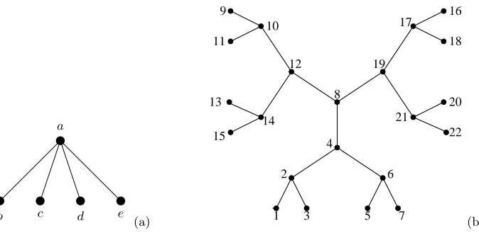
Example 11 1. LetT be the graph shown in Figure 2(a). The orderingb, a, c, d, e is a witness for lrw(T)≤1. The strategy for two cops according to the proof of Theorem 9 is as follows: the first cop moves tob and then the second cop moves toa and remains there. Now the first cop moves toc, d, e in this order. 2. The tree T in Figure 2(b) satisfies lrw(T) = 2. The given ordering (attached

to the vertices) witnesses lrw(T) ≤ 2. The strategy for three cops according to Theorem 9 is {1},{1,2},{2,3},{2,4},{4,5},{4,5,6},{4,6,7},{4,8},{8,9}, {8,9,10},{8,10,11},{8,10,12},{8,12,13},{8,13,14},{8,14,15},{8,16},{8,16,17}, {8,17,18},{8,17,19},{8,19,20},{19,20,21},{21,22}.

b

a

c _d e

(a)

18

3 1 14 9

8

17

20

22

7 5 4

2 6

13

15 11

10

19 12

21

16

[image:11.612.139.476.300.468.2]

(b)

Figure 2.The star of Example 11(1) and the tree of Example 11(2).

4 Linear Clique-Width and Path-Width

In this section we prove Theorem 3, characterizing the linear clique-width of trees in terms of their path-width.

Let us recall the definition of linear clique-width [14,19,31]. Letk be a positive integer. A k-labeled graph is a pair (G, γ) where Gis a graph and γ:V(G)→[k] is a mapping (that maps each vertex to one ofk labels); we will also denote it by (V(G), E(G), γ). Thek-labeled graph consisting of a single vertex labeled byi∈[k] is denoted by (i, γ_i). The set LIN-CWk of k-labeled graphs is defined inductively

with the following operations.

1. For eachi∈[k], (i, γi) is in LIN-CWk.

2. If i, j ∈[k] and (G, γ) is in LIN-CWk, then (ρi→j(G), γ′) is in LIN-CWk and

denotes thek-labeled graph (V(G), E(G), γ′_{) with}

γ′₍_x_{) :=}

(

(12)

3. Ifi, j ∈[k], i6=j, and (G, γ) is in LIN-CWk, then (ηi,j(G), γ) is in LIN-CWk

and denotes thek-labeled graph (V(G), E′_{, γ}_{) with}

E′_:=_E₍_G₎_{∪ {{}_{x, y}_{} |}_γ₍_x_{) =}_i_and_γ₍_y_{) =}_j_}_.

4. Ifi∈[k] and (G, γ) is in LIN-CWk, then (G⊕i, γ′) is in LIN-CWk and denotes

the graph (V(G)∪ {z}, E(G), γ′_{) where}_{z /}_∈_V₍_G_{) and}

γ′₍_x_{) :=}

(

γ(x) ifx∈V(G),

i ifx=z.

An expression built with the operations i, ρi→j, ηi,j and ⊕ according to the

definition of LIN-CWk is called a linear k-expression. The linear clique-width of

a graph G, denoted by lcw(G), is the minimum k such that G is isomorphic to a graph in LIN-CWk (after forgetting the labels). For example the linear

clique-width of a path of length 3 is 3. Note that if H is an induced subgraph ofG, then lcw(H)≤lcw(G). Moreover, any lineark-expressiontdefining a graphGdefines a linear ordering of V(G) witnessing the ordering in which the vertices of Gappear in t.

Lemma 12 ([10,14]) Any graphGsatisfieslcw(G)≤pw(G) + 2. ⊓⊔

Lemma 13 Let T be a tree obtained from three trees T1, T2 and T3 by adding a

new vertex r adjacent to one vertex in each of the three trees. If lcw(Ti) ≥k for each i∈ {1,2,3}, thenlcw(T)≥k+ 1.

Proof. Ifk= 1 then eachTi is a single vertex and henceT is a star with 3 leaves,

and we have lcw(T) = 2, because at least two different labels are necessary for adding an edge.

Assume that k > 1. This implies in particular, that each Ti has at least two

vertices. Let ℓ := lcw(T). We show thatℓ ≥k+ 1. Let t be a linear ℓ-expression definingT. and letπ:= (v1, . . . , vn) be the linear ordering ofV(T) corresponding to t. W. l. o. g. assume that the operations intare carried out in such a way, that each introduction of a new vertex v (operation type 1) is followed by a disjoint union (operation type 4), which in turn is followed by all possible edge additions involving

v (operations of type 3) and finally by recolorings that leave us with the smallest number of labels that is possible at this step [10, Proposition 2.101]. Moreover, we can assume that there is one distinguished label, theunlabel, that is assigned to a vertex once all its neighbors inT have been constructed (see for instance [33]).

Assume that v1 ∈/ V(T2) and vn ∈/ V(T2). Let π2 := u1, . . . , up be the linear

ordering ofV(T2) obtained by restrictingπtoV(T2) and lett2be the corresponding

subterm of t, which by the assumption above is a linear k-expression defining the treeT2. Let (X, Y) be a cut inπ2, whereXis partitioned into at leastklabel classes

(defined by the pre-images of the ≥k different labels), and assume that int2 we

cannot reduce the number of labels at (X, Y) by a recoloring operation. Such a cut exists because by assumption, lcw(T2) = k. If X is partitioned into more than k

label classes, then we are done, because then ℓ≥ k+ 1. Hence assume that X is partitioned into exactlyk label classes.

Choose a cut (X′_{, Y}′_{) of} _π _{such that} _X _⊆ _X′ _and _Y _⊆ _Y′_{. Since} _T _\_T

2 is

connected and by the choice oft2, there are two verticesxandysuch thatx∈X′\X,

y∈Y′_\_Y_{, and}_{_{x, y}_{} ∈}_E₍_T_{). Assume w.l.o.g that}_x_∈_V₍_T

1). Ify has no neighbor

in X, then, int, the vertexxcannot have the same label as any other vertex inX, and, sinceX is already partitioned intoklabel classes, this shows that ℓ≥k+ 1.

Assume now that there is a vertexz inX that is a neighbor of y. Theny =r,

(13)

rhas only one neighbor inT2and also one neighbor inT1. Now if one of the neighbors

ofzinT2is contained inY, thenxcannot have the same label as any other vertex

inX, and henceℓ≥k+ 1. Hence we may assume thatNT2(z)⊆X. Ifxandz have

different labels, then the label ofxmust be unique and ℓ≥k+ 1. Hence we may assume thatxandzhave the same label. Then no other vertex inX has this label. Towards a contradiction, suppose that at the cut (X′_{, Y}′_{) in} _t_{there are only} _k labels. If there is a vertexx′ _in_T

1with{x′} ∪NT(x′)⊆X′, then by the assumption

above x′ _{is labelled by the}_unlabel _in _t _{and we can reduce the number of labels at} the cut (X, Y) int2by assigning theunlabel toz(becausezdoes not have the same

label as any other vertex in X) – a contradiction to the choice of (X, Y). Hence every vertex inV(T1)∩X′has a neighbor inY′. Sincexandzhave the same label,

all the neighbors of NT1(x)⊆X

′_{. Using this and the fact that}_k _≥_{2, we see that} there exists at least one vertex x′ ₆₌_x_in _V₍_T

1)∩X′ and this vertex must have a

neighbor in Y′_{. But no vertex in} _T

2 can have the same label asx′. Again, we can

reduce the number of labels at the cut (X, Y) int2 by assigning the label of x′ to

z – a contradiction to the choice of (X, Y). Hence there are at leastk+ 1 labels at the cut (X′_{, Y}′_{) in}_t_{, proving that lrw(}_T₎_≥_k_{+ 1.} _⊓_⊔ We use the following Lemma, proved in [13, Theorem 3.1].

Lemma 14 ([13]) Let T be a tree and let k≥1 be an integer. Thenpw(T)≤k if and only if for allv∈V(T)at most two of the trees in T\v have path-widthkand

all others have path-width less thank. ⊓⊔

Lemma 15 Any treeT containing a path of length three satisfieslcw(T)≥pw(T) + 2. Proof. We use induction on k := pw(T). Ifk = 1 we are done because the linear clique-width of paths of length three is 3. If k= 2, then any tree of path-width 2 contains the treeR3obtained from the star with 3 leaves by subdividing once each

edge (cf. Figure 3), and by [22] lcw(R3) = 4. Now assume that for some k ≥ 2,

any tree having path-widthℓ≤k and containing a path of length three has linear clique-width at leastℓ+ 2. LetT be a tree that contains a path of length three and satisfies pw(T) =k+ 1. By Lemma 14 there exists a vertex r∈V(T) such that at least three trees inT\rhave path-width at leastk. Sincek≥2 each of these trees contain a path of length at least three, and by induction, these trees have linear clique-width at leastk+ 2 and hence by Lemma 13, lcw(T)≥k+ 3. ⊓⊔ Proof of Theorem 3. The first statement follows from Lemmas 12 and 15. For the second statement, if T does not contain a path of length three, then it is a star. Since stars with at least one edge have linear clique-width 2 and path-width 1, we can conclude that lcw(T) = pw(T) + 1. ⊓⊔

Before extending the result to forests, let’s warm up with some examples. The forestT consisting of two isolated edges satisfies lcw(T) = 3, while each of the con-nected components ofT has linear clique-width 2. Moreover, the forestT′_consisting of an isolated vertex and an isolated edge satisfies lcw(T′_{) = 2 (first construct the} edge), and the forestT′′_{obtained from}_T′ _{by adding a second isolated edge satisfies} lcw(T′′_{) = 3. For extending our results from trees to forests, we use the following} straightforward observation.

(14)

the connected components ofT assume the maximum of the linear clique-widths of the connected components of T, thenlcw(T)is equal to the maximum of the linear clique-widths of its connected components +1.

Proof. LetT1, T2, . . . , Tpbe the connected components ofT, and letk:= max{lcw(Ti)}.

Let t1, t2, . . . , tp be respectively the linear expressions defining T1, T2, . . . , Tp, and

lett′

i :=ρi→0(ti), where 0 is theunlabelcolor, that is never used to create an edge.

Lett:=tp⊕t′p−1⊕ · · · ⊕t′1. It is clear thatt definesT because the color 0 is never

used to create an edge. Assume T contains a path of length 3 and letT1, . . . , Tℓ be

the trees with a path of length 3. Then, for each 1≤i≤ℓ, lcw(Ti) = pw(Ti)+2 and tiuses surely theunlabel color, and forℓ+ 1≤i≤p, we have lcw(Ti) = pw(Ti) + 1.

Therefore, the linear expression tuseskcolors.

If any of theTi’s has a path of length 3, thenTis a disjoint union of stars andk=

2. Now, if lcw(T1) = 2, and lcw(Ti)≤1 for alli6= 1, thenL2≤i≤p1⊕(η1,2(1⊕2))

clearly defines T. Finally, if lcw(T1) = lcw(T2) = k = 2, then it is proved in [33]

that the linear clique-width ofT is 3. ⊓⊔

Corollary 1. There is a linear time algorithm that computes the linear clique-width of any n-vertex forest T, and a linear lcw(T)-expression can be computed in time O(n·log(n)).

Proof. From [13] there is a linear time algorithm that computes the path-width of any forest, and an optimal path-decomposition can be computed in time O(n·

log(n)) for every n-vertex forest. Hence, the statement follows from Observation 16 characterizing the linear clique-width of forests, and the proof of Lemma 12 in [10], which computes from an optimal path-decomposition (P, B) of widthka linear (k+2)-expression in timeO(max{k, ℓ}·n) whereℓis the maximum number of edges

in a bag of (P, B). ⊓⊔

5 Minimal Excluded Acyclic Vertex-Minors

As an application, in this section we identify the minimal excludedacyclic vertex-minors for linear rank-width kby using both Lemma 14 and Theorem 2.

For a graphGand a vertexxofG, thelocal complementation atxofGconsists in replacing the subgraph induced on the neighbors of xby its complement. The resulting graph is denoted byG∗x. IfH can be obtained fromGby a sequence of local complementations, then Gand H are calledlocally equivalent. A graphH is called avertex-minor of a graphGifHis isomorphic to a graph obtained fromGby applying a sequence of local complementations and deletions of vertices. The graph

H is aproper vertex-minor ofGifH is a vertex-minor ofGand|V(H)|<|V(G)|. A graph G is a minimal excluded vertex-minor for the class of graphs of linear rank-width k, if lrw(G)> k and lrw(H)≤kfor all proper vertex-minors H ofG. See [8,24] for more information on vertex-minors.

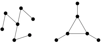
We say that a graphGis aminimal excluded acyclic vertex-minorfor the class of graphs of linear rank-widthk, ifGis acyclic and every proper acyclic vertex-minor ofGhas linear rank-width less thank. Note that a minimal excluded acyclic vertex-minor may not be a minimal excluded vertex-vertex-minor. For example,R3of Figure 3 is

a minimal excluded acyclic vertex-minor for the class of graphs of linear rank-width at most 1, but it contains the net graph, also of Figure 3, as a proper vertex-minor, which in turn is a minimal excluded vertex-minor for the class of graphs of linear rank-width at most one [1].

(15)

[image:15.612.218.398.97.177.2]

Figure 3.The subdivided 3-starR3, and the net graph.

Let H1 :={R3}. For k ≥2, let Hk be the set of (pairwise non isomorphic) trees

obtained by taking a new vertexrand three trees inHk−1, and by linking this new

vertex to one vertex in each of these three trees. Notice that all the trees in Hk

have the same size. ByRk we denote the set of (pairwise non isomorphic) treesT′

obtained from treesT ∈ Hk by adding a new vertex adjacent to one vertex ofT. A rooted tree inHk∪ Rk is a treeT inHk∪ Rk rooted at some vertex.

A rooted tree H is a rooted vertex-minor of a rooted tree G if H is a vertex-minor ofG,H is obtained without applying a local complementation at the root of

Gand the root ofH is mapped to the root ofG. We recall that ifT is a rooted tree andv is a vertex ofT then we denote byTv _{the subtree of}_T _{rooted at}_v_.

Lemma 17 Letk≥2and letT be a rooted tree of linear rank-widthk. Let2≤ℓ≤ k and letv ∈V(T)be such that Tv _{has linear rank-width} _{ℓ. Then} _Tv _{has a rooted} tree inHℓ−1∪ Rℓ−1 as a rooted vertex-minor.

Proof. We prove it by induction onℓ. Letv be such thatTv _{has linear rank-width}

2. By Lemma 14 there exists a vertex u in Tv _{such that} _Tu _{is isomorphic to a}

rooted star, rooted at its center, by subdividing at least once three of its edges. LetH be the rooted subtree ofTv _{induced by the vertices in the path from}_v _to_u

and three paths of length two originated fromu. It is clear thatHu _{is isomorphic}

to a rooted tree in H1 (by taking in the tree in H1 the vertex of degree three as

root). Now it is clear that H admits a rooted tree inH1∪ R1 as a rooted

vertex-minor by applying local complementations at intermediate vertices in the path from

v to uand removing them after each local complementation. Since H is a rooted vertex-minor ofTv_{, we are done.}

Now assume the claim is true for all vertices v of T such that Tv _{has linear}

rank-width at mostℓ′_{and let}_u_{be a vertex of}_T _{such that}_Tu_{has linear rank-width} ℓ′_{+ 1. By Lemma 14 there exists a vertex} _v _in _Tu _{such that} _Tv _{has linear}

rank-widthℓ′_{+ 1 and three neighbors} _v

1, v2 andv3such thatTvi has linear rank-width

ℓ′_{. By inductive hypothesis for each} _i _{∈ {}₁_,₂_,₃_} _{there exists a rooted tree} _H

i in Hℓ′₋₁∪R

ℓ′₋₁such thatH

iis a rooted vertex-minor ofTvi. For eachi∈ {1,2,3}the

local complementations applied to obtainHi do not modify the tree inT\Tvi. So

the rooted tree obtained fromTv_{and composed of the}_H

is and of the paths fromu

to thevis is a rooted vertex-minor ofTu. We obtain a tree inHℓ′∪ R

ℓ′ as a rooted

vertex-minor ofTu_{as follows. If}_H

iis inRℓ′₋₁, then apply a local complementation

at vi, and then remove vi. In this way, we get a vertex-minor of Tv rooted at v

and isomorphic to a rooted tree in Hℓ′. By applying local complementations at

intermediate vertices in the path fromv to uand removing them after each local complementation we get a rooted tree inHℓ′∪ R_ℓ′ as a rooted vertex-minor ofTu.

⊓ ⊔

(16)

Proof. Let T be a tree with linear rank-width k+ 1. By Theorem 2 and Lemma 14 there exists a vertex r and three trees T1, T2 and T3 of T \r such that each

Ti has linear rank-widthk and has a vertexri adjacent tor. Let F :=T[V(T1)∪

V(T2)∪V(T3)∪ {r}], which is a subtree ofT. Notice that by Lemma 14F has linear

rank-width k+ 1. Let us rootF in r and letr1, r2 andr3 denote the neighbors of

r in F. By Lemma 17 each Ti has a rooted tree Hi in Hk−1∪ Rk−1 as a rooted

vertex-minor. Then the treeF′ _{composed of the rooted trees}_H

is and of the edges {r, ri}is a rooted vertex-minor ofF. We obtain a tree inHk fromF′ as follows. If Hiis inRk−1, then apply a local complementation atri, and then removeri. Since

we can do each local complementation independently, we are done. ⊓⊔

Theorem 19 For each k ≥ 1, the set Hk is the set of minimal excluded acyclic vertex-minors for linear rank-width k.

Proof. One can prove by induction, by using Theorem 2 and Lemma 14, that each tree in Hk has linear rank-width k+ 1 and is minimal (as a tree) with respect to

this property. Moreover, by Lemma 18 any tree of linear rank-widthk+ 1 contains as a vertex-minor a tree inHk. So it is enough to prove that two trees inHk are not

locally equivalent. Bouchet has proved in [8] that two trees are locally equivalent if and only if they are isomorphic. Hence, since no two trees inHk are isomorphic, we

are done. ⊓⊔

Notice that Theorem 19 is another unexpected relation between linear rank-width and path-rank-width of trees. In fact, as proved in [38] the set Hk is also the set

of acyclic (topological) minor obstructions for path-width k.

6 Conclusion

We proved that linear rank-width and path-width coincide on forests, and we de-termined the linear clique-width of forests in terms of their path-width. While the proof of the former result uses a game characterization of path-width, the proof of the latter is based on a Lemma 13 which gives a recursive characterization of the linear clique-width of trees (similar to Lemma 14 for path-width of trees). Indeed, linear rank-width can be characterized recursively in a similar way [26, Lemma 4.1], and this characterization can be used to prove the equality of linear rank-width and path-width on forests. Our characterizations imply the existence of linear time al-gorithms for computing the linear rank-width and the linear clique-width of forests. The recent paper [3] gives a polynomial time algorithm for computing the linear rank-width of distance-hereditary graphs. It is still wide open, whether a similar re-sult can be obtained for computing linear clique-width. More generally, it is natural to ask whether there is a polynomial time algorithm for computing linear rank-width (or path-rank-width or linear clique-rank-width) on graphs of bounded rank-rank-width. It is also open, whether there is a polynomial time algorithm that computes linear rank-width (or linear clique-width) on series-parallel graphs.

It should be possible to extend our methods to characterize linear NLC-width (cf. [19]) of trees in terms of their path-width (similar to Theorem 3), but it seems harder to identify the exceptions (as the stars for clique-width) and the basic graphs to start the induction (as the R3 graph).

(17)

excluded vertex-minors for linear rank-width k (we know from [25] and [3] that their number is doubly exponential in k). In [24] it is proved that the size of the excluded vertex-minors for rank-width k is bounded by (6k+1₋₆₎_/_{5, and similar}

results exist for tree-width and path-width [30]. Can we get a similar result for linear rank-width? Such a bound would prove the existence of an effective algorithm for checking whether a graph has linear rank-width at most k, for fixed k, while we only know from [34] that an algorithm exists.

Contrary to (linear) rank-width (linear) clique-width is not monotone with re-spect to vertex-minor inclusion. For example, the pathP on three edges has (linear) clique-width 3, while the graphGobtained fromP by a local complementation at a vertex of degree 2 inP is a triangle with a pendant edge, andGhas (linear) clique-width 2. Characterizing linear clique-clique-width with respect to the induced subgraph inclusion seems to be a hard task and few results have been obtained [17,23]. Can we at least characterize the linear width of co-graphs (which have clique-width at most 2) or, more generally, of distance-hereditary graphs (which have clique-width at most 3) in order to identify the set of distance-hereditary excluded induced subgraphs for linear clique-widthk?

The characterizations of linear rank-width and linear clique-width of forests in terms of their path-width are surprising. However, we believe that forests are ex-ceptional and, except for special types of graphs (e. g. grids), such characterizations are not to be expected. But we believe that the results in this paper can be used to (approximately) compute the linear rank-width or clique-width of tree-like graphs.

References

1. Isolde Adler, Arthur M. Farley, and Andrzej Proskurowski. Obstructions for linear

rank-width at most 1. Discrete Applied Mathematics, 168:3–13, 2014.

2. Isolde Adler and Mamadou Moustapha Kanté. Linear rank-width and linear clique-width of trees. In Andreas Brandstädt, Klaus Jansen, and Rüdiger Reischuk, editors,

WG, volume 8165 ofLecture Notes in Computer Science, pages 12–25. Springer, 2013.

3. Isolde Adler, Mamadou Moustapha Kant´e, and O.-joung Kwon. Linear rank-width

of distance-hereditary graphs. In Dieter Kratsch and Ioan Todinca, editors,

Graph-Theoretic Concepts in Computer Science - 40th International Workshop, WG 2014. Revised Selected Papers, volume 8747 ofLecture Notes in Computer Science, pages 42–55. Springer, 2014.

4. Daniel Bienstock, Neil Robertson, Paul D. Seymour, and Robin Thomas. Quickly excluding a forest. J. Comb. Theory, Ser. B, 52(2):274–283, 1991.

5. Hans L. Bodlaender and Ton Kloks. Efficient and constructive algorithms for the

pathwidth and treewidth of graphs. J. Algorithms, 21(2):358–402, 1996.

6. Hans L. Bodlaender, Ton Kloks, and Dieter Kratsch. Treewidth and pathwidth of

permutation graphs. SIAM J. Discrete Math., 8(4):606–616, 1995.

7. Hans L. Bodlaender and Rolf H. M¨ohring. The pathwidth and treewidth of cographs.

In John R. Gilbert and Rolf G. Karlsson, editors,SWAT, volume 447 ofLecture Notes

in Computer Science, pages 301–309. Springer, 1990.

8. Andr´e Bouchet. Transforming trees by successive local complementations. J. Graph

Theory, 12(2):195–207, 1988.

9. Andr´e Bouchet. Circle graph obstructions. J. Comb. Theory, Ser. B, 60(1):107–144,

1994.

10. Bruno Courcelle and Joost Engelfriet. Graph Structure and Monadic Second-Order

Logic, A Language-Theoretic Approach. Cambridge University Press, 2012.

11. Bruno Courcelle and Stephan Olariu. Upper bounds to the clique width of graphs.

Discrete Applied Mathematics, 101(1-3):77–114, 2000.

12. Nick D. Dendris, Lefteris M. Kirousis, and Dimitrios M. Thilikos. Fugitive-search

games on graphs and related parameters. Theor. Comput. Sci., 172(1-2):233–254,

(18)

13. Jonathan A. Ellis, Ivan Hal Sudborough, and Jonathan S. Turner. The vertex sepa-ration and search number of a graph.Inf. Comput., 113(1):50–79, 1994.

14. Michael R. Fellows, Frances A. Rosamond, Udi Rotics, and Stefan Szeider.

Clique-width is np-complete.SIAM J. Discrete Math., 23(2):909–939, 2009.

15. Robert Ganian. Thread graphs, linear rank-width and their algorithmic applications. In Costas S. Iliopoulos and William F. Smyth, editors,IWOCA, volume 6460 ofLecture Notes in Computer Science, pages 38–42. Springer, 2010.

16. Chris Godsil and Gordon Royle.Algebraic graph theory, volume 207 ofGraduate Texts

in Mathematics. Springer-Verlag, New York, 2001.

17. Frank Gurski. Characterizations for co-graphs defined by restricted nlc-width or

clique-width operations.Discrete Mathematics, 306(2):271–277, 2006.

18. Frank Gurski. Linear layouts measuring neighbourhoods in graphs. Discrete

Mathe-matics, 306(15):1637–1650, 2006.

19. Frank Gurski and Egon Wanke. On the relationship between nlc-width and linear nlc-width.Theor. Comput. Sci., 347(1-2):76–89, 2005.

20. Frank Gurski and Egon Wanke. The nlc-width and clique-width for powers of graphs

of bounded tree-width. Discrete Applied Mathematics, 157(4):583–595, 2009.

21. Pinar Heggernes, Daniel Meister, and Charis Papadopoulos. A complete characterisa-tion of the linear clique-width of path powers. In Jianer Chen and S. Barry Cooper,

editors,TAMC, volume 5532 ofLecture Notes in Computer Science, pages 241–250.

Springer, 2009.

22. Pinar Heggernes, Daniel Meister, and Charis Papadopoulos. Graphs of linear

clique-width at most 3.Theor. Comput. Sci., 412(39):5466–5486, 2011.

23. Pinar Heggernes, Daniel Meister, and Charis Papadopoulos. Characterising the linear

clique-width of a class of graphs by forbidden induced subgraphs. Discrete Applied

Mathematics, 160(6):888–901, 2012.

24. Sang il Oum. Rank-width and vertex-minors.J. Comb. Theory, Ser. B, 95(1):79–100,

2005.

25. Jisu Jeong, O.-joung Kwon, and Sang-il Oum. Excluded vertex-minors for graphs of linear rank-width at most k. Eur. J. Comb., 41:242–257, 2014.

26. O joung Kwon. Connecting rank-width and tree-width via pivot-minors, 2012. Master’s Thesis.

27. Nancy G. Kinnersley. The vertex separation number of a graph equals its path-width.

Information Processing Letters, 42(6):345 – 350, 1992.

28. Lefteris M. Kirousis and Christos H. Papadimitriou. Searching and pebbling. Theor.

Comput. Sci., 47(3):205–218, 1986.

29. Ton Kloks and Hans L. Bodlaender. Approximating treewidth and pathwidth of some classes of perfect graphs. In Toshihide Ibaraki, Yasuyoshi Inagaki, Kazuo Iwama,

Takao Nishizeki, and Masafumi Yamashita, editors, ISAAC, volume 650 of Lecture

Notes in Computer Science, pages 116–125. Springer, 1992.

30. Jens Lagergren. Upper bounds on the size of obstructions and intertwines. J. Comb.

Theory, Ser. B, 73(1):7–40, 1998.

31. Vadim V. Lozin and Dieter Rautenbach. The relative clique-width of a graph. J.

Comb. Theory, Ser. B, 97(5):846–858, 2007.

32. Nimrod Megiddo, S. Louis Hakimi, M. R. Garey, David S. Johnson, and Christos H.

Papadimitriou. The complexity of searching a graph. J. ACM, 35(1):18–44, 1988.

33. Daniel Meister. Clique-width with an inactive label.Discrete Mathematics, 337:34–64, 2014.

34. Sang-il Oum. Approximating rank-width and clique-width quickly.ACM Transactions

on Algorithms, 5(1), 2008.

35. Sang-il Oum and Paul D. Seymour. Approximating clique-width and branch-width.

J. Comb. Theory, Ser. B, 96(4):514–528, 2006.

36. Petra Scheffler. Die Baumweite von Graphen als ein Maß f¨ur die Kompliziertheit

algorithmischer Probleme. Akademie der Wissenschaften der DDR, Berlin, 1989. PhD thesis.

37. Karol Suchan and Ioan Todinca. Pathwidth of circular-arc graphs. In Andreas

(19)

38. Atsushi Takahashi, Shuichi Ueno, and Yoji Kajitani. Minimal acyclic forbidden minors

for the family of graphs with bounded path-width. Discrete Mathematics,

127(1-3):293–304, 1994.