City, University of London Institutional Repository
Citation:
Alam, S. S. & Jianu, R. (2016). Analyzing Eye-Tracking Information in
Visualization and Data Space: from Where on the Screen to What on the Screen.. IEEE
Transactions on Visualization and Computer Graphics, PP(99), doi:
10.1109/TVCG.2016.2535340
This is the accepted version of the paper.
This version of the publication may differ from the final published
version.
Permanent repository link:
http://openaccess.city.ac.uk/15527/
Link to published version:
http://dx.doi.org/10.1109/TVCG.2016.2535340
Copyright and reuse: City Research Online aims to make research
outputs of City, University of London available to a wider audience.
Copyright and Moral Rights remain with the author(s) and/or copyright
holders. URLs from City Research Online may be freely distributed and
linked to.
City Research Online:
http://openaccess.city.ac.uk/
[email protected]
Analyzing Eye-Tracking Information in
Visualization and Data Space: from Where on
the Screen to What on the Screen
Sayeed Safayet Alam
∗,
Member, IEEE,
and Radu Jianu
†,
Member, IEEE
Abstract—Eye-tracking data is currently analyzed in the image space that gaze-coordinates were recorded in, generally with the help of overlays such as heatmaps or scanpaths, or with the help of manually defined areas of interest (AOI). Such analyses, which focus predominantly on where on the screen users are looking, require significant manual input and are not feasible for studies involving many subjects, long sessions, and heavily interactive visual stimuli. Alternatively, we show that it is feasible to collect and analyze eye-tracking information in data space. Specifically, the visual layout of visualizations with open source code that can be instrumented is known at rendering time, and thus can be used to relate gaze-coordinates to visualization and data objects that users view, in real time. We demonstrate the effectiveness of this approach by showing that data collected using this methodology from nine users working with an interactive visualization, was well aligned with the tasks that those users were asked to solve, and similar to annotation data produced by five human coders. Moreover, we introduce an algorithm that, given our instrumented visualization, could translate gaze-coordinates into viewed objects with greater accuracy than simply binning gazes into dynamically defined AOIs. Finally, we discuss the challenges, opportunities, and benefits of analyzing eye-tracking in visualization and data space.
F
1
I
NTRODUCTIONE
YE-tracking allows us to locate where users are looking on a computer screen [1], [2] and is often used to record peoples’ gazes while they are performing tasks that involve visual stimuli, and to analyze this data off-line to see how people interpreted the stimuli and solved the tasks [3]. Diagnostic eye-tracking has been used widely in psychology and cognitive science to help researchers understand thought and affect mechanisms [4], and in data visualization and human computer interaction (HCI) to explain how people use visual interfaces [3].To date, eye-tracking data is collected and interpreted in a low-level form, as gaze-coordinates in the space of rendered visual stimuli that gazes were recorded for. Relating this data to the semantic content of the stimuli is generally done offline by human analysts or coders who inspect gaze heatmaps visually, or define area of interest (AOIs) manually. As such, this process requires significant manual intervention and is especially difficult for studies involving many subjects, long sessions, and interactive content.
The work we describe here rests on the observation that for visual content that a computer generates on the fly, such as data visualizations, the structure and layout of the visual content is known at rendering time. Thus, for data visualizations with source code that is open to instrumentation, gaze-coordinates provided by an eye-tracker can be related to the rendered content of the visu-alization in real-time, yielding a detailed account of visuvisu-alization
• ∗S. S. Alam is with the School of Computing and Information Sciences, Florida International University, Miami, FL, 33199.
E-mail: [email protected]
• † R. Jianu is with the School of Computing and Information Sciences, Florida International University, Miami, FL, 33199.
E-mail: [email protected]
Manuscript received April 19, 2005; revised September 17, 2014.
elements, and implicitly data elements, that users are viewing. Our paper shows that this instrumentation approach is indeed feasible and produces data that can be collected over long sessions involving open-ended tasks and interactive content. Moreover, the collected data is derived directly from the visualization’s underlying data, and thus has semantic meaning without the need for additional coding. As such, this data can be particularly well suited to explain how people forage for, analyze, and integrate information in complex visual analytics systems and workflows.
While this idea is similar to previous work on 3D objects of interest (OOI) [5], and dynamic AOIs [6], detecting individual data and visualization objects that are being viewed (e.g., nodes in a network) is different than binning gazes into AOIs, which are traditionally large, non-overlapping, and lack data-derived semantic meaning. Instead, we evaluate the feasibility of collecting data that is highly granular and has semantic meaning. This creates interesting opportunities for data analysis, which we exemplify in Section 4 and discuss in Section 5, but also involves a challenge: how can we accurately use eye-tracking data, which is generally imprecise and low resolution, to discriminate between many small, intertwining visual objects which are typical of data visualization content?
a given time [7], [8]. We contribute by introducing and evaluating an algorithm that can “intelligently” detect viewed objects from gaze coordinates in real-time and that is tailored to visualization content, and we reveal and quantify viewing patterns such as those described above for one specific visualization.
To evaluate the feasibility of collecting and analyzing eye-tracking data directly in visualization and data space, we used the aforementioned algorithm to instrument an interactive visual-ization of IMDB data and collect viewed-object data from nine subjects. We then showed that the instrumentation yielded useful results in two ways. First, we show that viewed objects identified by our instrumentation method are tightly related with tasks we asked users to do. Second, we show that differences between the manual annotations of five coders who were asked to analyze the raw gaze data, and our automatically collected data, are not greater than differences between the coders’ own annotations. As part of this quantitative evaluation, we also show that our novel algorithm for detecting viewed objects outperforms two na¨ıve implementations.
Our contributions are: (i) a qualitative and quantitative demonstration of the validity, effectiveness, and potential of an-alyzing eye-tracking data in visualization and data space; (ii) an “intelligent” algorithm for detecting viewed objects from eye-tracking data in visualizations that are open for instrumentation, and its quantitative evaluation; (iii) a demonstration of the ex-istence of viewing patterns in visualization and a methodology to compute them; (iv) a discussion of methods, benefits, and applications for collecting and analyzing eye-tracking data in visualization and data space.
2
R
ELATEDW
ORKEye-tracking can locate users’ gazes on a computer screen [1], [2] and is a technology that is becoming increasingly accurate, fast, and affordable [3], [9]. Eye-tracking is often used to record peoples’ gazes while performing tasks that involve visual stimuli, and to analyze the data off-line to gain insight into how people interpreted the stimuli and solved the tasks [3]. For example, eye-tracking was used to understand how people perceive faces [10], [11], to study how attention changes with emotion [12], to under-stand changes in perception that are caused by disease [13], and to gain insight into how students use visual content to learn [14], [15], [16], [17]. Within the field of data visualization, examples of eye-tracking studies include but are not limited to work by Pohl et al. and Huang et al. on graph readability [18], [19], [20], Burch et al.’s work on tree-drawing perception [21], [22], and work by Kim et al. on evaluating an interactive decision making visualization [23].
Eye-tracking data is traditionally interpreted and analyzed in the space of rendered visual stimuli that gazes were recorded for, using one of two analysis paradigms: point based or area of interest (AOI) based [24]. Point based analyses treat gaze samples or fixations as independent points while AOI analyses first aggregate gazes into areas of interest and then operate at this higher level of abstraction. Most often, experimenters define AOIs manually, but gaze clustering algorithms are also available to automatically define AOIs based on the available eye-tracking data [25], [26], [27].
Our work is closest to a sparse set of methods that seek to automatically relate gazes to the semantics of computer generated content. Several papers allude to the fact that AOIs could be
defined dynamically for such cases [28], [29], but none formalize an approach or quantify feasibility. More concretely, for dynamic stimuli with known 3D structure, researchers have explored the concept of objects of interest (OOI), in which gazes are auto-matically assigned to 3D objects in the scene [5]. More recently, Bernhard et al. looked at similar gaze-to-object mapping in the context of understanding what people were looking at in virtual 3D environments [30]. Our work presents a more detailed account of how gazes can be automatically assigned to content typical of 2D information visualizations and evaluate how effective this can be.
Moreover, our method of detecting viewed objects improves over na¨ıve methods by leveraging Salvucci’s “intelligent gaze interpretation” paradigm [7], [8]. Specifically, Salvucci found that simply assigning gazes to an object if the gazes’ coordinates are within the bounds of the object is insufficient, and that leveraging the semantics of visual content can significantly improve our ability to predict which objects are viewed. More recently, Okoe et al. found similar results, albeit using a different method [31], [32]. We extend on such work by presenting an intelligent gaze interpretation’ algorithm that is tailored to content typical of data visualization and by evaluating it.
Finally, the visualization community proposed a plethora of visualization and visual analytics tools for both point-based and AOI based eye-tracking analysis. Blascheck et al. provides a com-prehensive review of such methods [24]. Most relevant to our work are methods for AOI visualization, since our data is in essence a highly granular and annotated AOI data. Popular examples of such techniques include scarf plots [33], AOI rivers [34], and AOI transition matrices [35]. Also relevant are visual analytics principles and systems for analyzing AOI data, such as work by Andrienko et al. [36], Weibel et al. [37], and Kurzhals et al. [29]. However, the data our instrumentation allows us to collect differs from regular AOI data through its high granularity, connection with the underlying data of visualizations, and uncertainty about whether an object AOI was truly viewed. Moreover, the focus of the work we present here is not in proposing novel techniques of analyzing data collected in visualization and data space, but on whether and how this can be done accurately and whether it is beneficial.
3
M
ETHODSabout these changes as soon as the visualization is redrawn and will map subsequent gaze samples to the new visual layout.
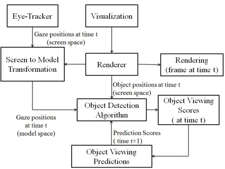
Fig. 1: Real-time detection of viewed objects in generative visual-izations.
Next, we describe an effective algorithm for mapping gaze samples to objects that users are viewing. As shown in Figure 1, we will assume that gaze samples have already been transformed from screen space into model space. As such, the basic input of our algorithm is a stream of gaze samples in model space, and a list of visual primitives drawn on the screen, together with their shape and position. Naturally, as most modern visualizations are interac-tive, this visual structure of the visualization is likely to be highly dynamic. The algorithm outputs a stream of viewed visualization and data primitives (e.g., nodes, labels) in real-time, as users are viewing them in the instrumented visualization. Of course, our approach is limited in that it cannot be applied to already rendered images or videos and requires that the visualization’s source code can be altered. We discuss these limitations in Section 5.3.
We will describe our algorithm incrementally in the following three sections, starting from a na¨ıve approach that simply draws AOIs dynamically around visualization objects, to a predictive one that detects objects more accurately by using knowledge about how specific visualizations are typically used. A comparative evaluation of these three object detection algorithms is presented in Section 4.2.1.
3.1 Algorithms for viewed object detection in data vi-sualizations
3.1.1 AOI-based viewed object detection
A na¨ıve viewed object detection approach is to treat object shapes as dynamic AOIs and determine that a viewed object is that with the most recent fixation landing in its AOI. This is a natural first try at detecting viewed visual objects from gaze data automatically, given that manually drawn AOIs are typically used in the same manner in offline eye-tracking data analysis, and that the similar concept of objects of interest (OOIs) has been proposed already by Stellmach et al. [5] for generative 3D content.
The problem with this approach is that for highly granular visual content, such as individual nodes or labels, users often fixate in the vicinity of the object rather than on the object itself. We demonstrate and quantify this observation in Section 4. A potential solution to this problem could be to make object AOIs slightly
larger than the objects themselves. However, larger AOIs may lead to AOI overlap in cluttered visualizations and to the inability to assign a gaze sample or fixation to any single AOI. Ultimately, the problem lies with an inability to determine with absolute certainty what a user is looking at, and is described in more detail in the next section.
3.1.2 A probabilistic approach to viewed object detection
Unlike mouse input, eye-tracking can only indicate a small screen region that a user is fixating, rather than a particular pixel. Typically, such a region is about one inch in diameter, though specific values depend on the user’s distance to the monitor, and is determined by how human vision works. As such, we argue that it is generally impossible to tell with absolute certainty which object a user is viewing, if the user is fixating in the vicinity of multiple close objects (Figure 2(a)). This is not a significant problem for traditional AOI analyses, which generally use large AOIs. However, our goal is to detect the viewing of granular visual content, such as network nodes or glyphs, in cluttered visualizations.
Fig. 2: (a) A real visualization example in which a user fixates in the vicinity of multiple close object groups (red dot). (b) predictive method: even though the latest gaze sample falls equidistantly between visual objectsO3andO4, we suspect thatO3is the more
likely viewing target given that (i) it is highlighted, and (ii) it is connected toO1, which is likely to have been the object that the
user viewed previously (vs1=0.6>vs2=0.4).
As such, we advocate for a fuzzy interpretation of gaze data and detecting likelihoods that objects are viewed rather than certainties. To this end, we can compute object gaze scores gs
(for all objectsiin a visualization, and at all timest) that range between zero- the object is not viewed, and one- the object is certainly viewed as shown in Figure 3 and Formula 1.
gsi,t=1−min(1,(
d
R)) (1)
[image:4.612.312.564.284.455.2]Fig. 3: Calculating a gaze scoregsfor a given object and a gaze sample landing nearby, wheredis the distance from the object to the gaze sample, andRapproximates the size of the user’s foveated region.
Finally, we note that the object scores (gs) do not directly equate to probabilities. The distinction is important because it implies that our implementation can detect two objects as being viewed simultaneously (gs1=1 and gs2=1). We think this is
appropriate since a person can in fact visually parse multiple objects at the same time if they fall within the user’s foveated region, and even think of multiple objects as a unit for specific task purposes. We discuss this in more detail in Section 5.5.
3.1.3 A predictive algorithm for viewed object detection in data visualization
Salvucci and Anderson described the concept of “intelligent gaze interpretation” in the context of a gaze-activated interface [8]. Their method achieved better accuracy in detecting which inter-face control a user is gazing at, by integrating both the proximity of the gaze to the control, and the likelihood that the control would be the target of a gaze-interaction, based on the current state and context of use of the interface. Formally, their algorithm identifies the most likely currently viewed itemiviewedby solving
iviewed=argmax
i∈I
[Pr(g|i)·Pr(i)]
wherePr(g|i)is the probability of producing a gaze at location
g given the intention of viewing item i, and Pr(i) is the prior probability of an item i being the target of a gaze-interaction. In Salvucci and Anderson’s proof of concept implementation these prior probabilities were based on assumptions about how an interface might be used and were hardcoded into the system.
We adapt Salvucci and Anderson’s paradigm to more accu-rately determine which object a user is viewing, in the ambiguous case when a gaze-sample lands close to multiple objects (e.g., Figure 2(a).
For example, in a network visualization we may assume that a user who has just viewed a nodenwill more likely view one ofn’s neighbors than a random other node, perhaps especially if the user previously highlighted nodenand its outgoing edges. In Section 4 we show qunatitatively that this assumption is in fact true for one visualization we tested.
We consider a simplified such scenario in Figure 2(b): four visual objects (O1...4), two of which are connected (O1 andO3),
and one of which is highlighted (O3), are shown on the screen. A
new gaze sample registers betweenO3andO4at timet. Intuitively,
it is more likely that O3 was viewed since it is highlighted.
Moreover, if we knew thatO1 was viewed just before the current
moment, and, as described above we assume that users generally view neighboring nodes together, then this likelihood becomes even stronger.
Formally, we compute vsi,t (i.e., the viewing score vs of
objecti at timet) by weighing the gaze scoregsi,t described in
Section 3.1.2 by a prediction scorepsi,tthat objectiis a viewing
target at timet:
vsi,t=gsi,t×psi,t (2)
This prediction score is computed based on the likelihood that the object is viewed given the current state of the visualization (e.g., the object is highlighted), and the likelihood that it is viewed if some other specific object (e.g., a node’s neighbor) was viewed just before it. Those two components are formalized by the α
score andβscore in Formula 3, and are described below.
psi,t=αi,t×βi,t (3)
First, we will assumeα is given as an input to our algorithm. Concrete examples of whatα could be linked to are whether an object is highlighted (larger alpha) or not, whether an object is part of a group of objects recently queried by the user, or whether an object is known to be of particular interest to the users’ current workflow (e.g., because they have viewed it often before, because the visualization was constructed using those objects as initial seeds, because they are mentioned as keywords in a user’s profile). Second, we will compute β based on a viewing transition functionTbetween objects:T(j,i)gives the likelihood that object
i is viewed after object j is viewed. We will again assume that
T(j,i)is given as input to our algorithm. Concrete examples of what T(j,i)could be linked to are whether objects i and j are somehow connected or related. This connection could be either visual, such as an explicit edge or leader line or an implicit sharing of similar visual attributes (e.g., color, shape), or semantic (e.g., both nodes are actors).
To computeβ, we could considerβi,t=T(j,i)but that would
involve knowing j, the previously viewed object, with absolute certainty. This is problematic because we often cannot unequiv-ocally determine which item was viewed at any given time. For example, as illustrated in Figure 2(b),O1’s previous viewing score
(vs1,t−1 =0.6), is just slightly larger than O2’s viewing score
(vs2,t−1 =0.4), and thus an absolute choice of O1 over O2 as
previously viewed element would be rather arbitrary. In other words, we cannot say with absolute certainty which of the two objects was viewed before because the user fixated between them. In more general terms, our computation of βi,t must account
for multiple items j that may have been viewed before. These itemsjare those with a previous visual scorevsj,t−1that is greater
than 0. As such, we compute βi,t as a weighted average of all
transition probabilities from objects j with vsj,t−1>0 , to our
current item i. The weights are given exactly by the likelihood that an object jwas viewed before - in other words by its previous viewing scorevsj,t−1. This computation is captured by Formula 4.
βi,t=
∑
j
vsj,t−1×T(j,i)
∑
j
vsj,t−1
, where
0≤i≤nandgsi,t>0
0≤j≤nandvsj,t−1>0
0≤j≤nandgsj,t=0
of. For example, in our simplified scenario, usingO3as a previous
element in a competition between itself and O4 would result in
an open feedback-loop and should be avoided. This restriction is reflected in Formula 4 by the 3rd inequality. The algorithm pseudocode is provided in Algorithm 1.
Algorithm 1Viewed Object Detection Algorithm
1: Inputs:
Oi,...,n= tracked visualization objects (shapes, positions)
g(x,y) =gaze sample in model space (timet)
αi,...,n=view weights (αi,...,n∈[0,1])
T(i,j) =viewing transition function (T(i,j)∈[0,1])
2: Outputs:
vsi,t=momentary viewing scores of all objects (i=1, . . . ,n).
3: fori←1 tondo
4: Computegsi,tusing Formula 1
5: max←0
6: fori←1 tondo
7: ifgsi,t>0then
8: Computeβi,tusing Formula 4 9: ps′i,t←αi,t×βi,t
10: ifps′i,t>maxthen
11: max←ps′i,t
12: fori←1 tondo
13: vsi,t←gsi,t× ps′i,t max
Lastly, we note two more factors. First, to optimize for speed, we only compute prediction scores for objects with non-zero gazes (Algorithm 1, line 7). Second, in our implementation we compute viewing scores for every gaze sample, rather than every fixation. We believe that doing so leads to results that are less dependent on how fixations are computed and more robust. Since our eye-tracker’s sampling rate is 120Hz, the scoresvsj,t−1were
computed just 8ms ago, an interval generally shorter than the time it takes for people to shift their attention to a new object. As such, instead of using the rawvsj,t−1score, we use an average of
the last several viewing scores, and, for all practical purposes, the term vsj,t−1 should be replaced in the previous formulas
by∑kk==151 vsj,t−1, which, given our eye-tracker’s 120Hz temporal
resolution, averages samples over approximately 125ms, a time window we observed to be close to an average fixation duration.
However, we note that our algorithm can take as input fixations rather than individual gaze samples, in which case this step would not be necessary. Moreover, additional smoothing and filtering such as those summarized by Kumar et al. [38] could be used as a pre-processing step to clean gazes before feeding them into our algorithm. For example, we tried removing gaze samples with high velocity as they are likely to be part of saccades, but observed no discernable improvement in our algorithm’s output.
Performance analysis:The algorithm needs to swift through all tracked elements (n) to find those in the proximity of a gaze sample or fixation (kt). Then, to compute the term β for each
of the kt potentially viewed elements, the algorithm will iterate
overkt−1objects with non-zero viewing scores from the previous
iteration. As such, the algorithm is linear if we consider the number of objects that a user can view at any time to be a constant. However, that is not necessarily true since in special cases the entire visualization may fall within the algorithm’s R
radius (e.g., the visualization is zoomed out too much). However, in this case the output of the algorithm would be irrelevant anyway
and the algorithm should not be run. Thus, the algorithm is limited primarily by the clutter of the visualization, rather than the amount of computation.
3.2 Instrumenting a concrete visualization
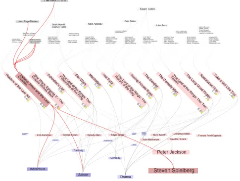
We have used the previously described principles to instru-ment Doerk’s interactive PivotPaths visualization of multifaceted data [39], which we linked to the popular internet movie database (IMDB). Shown in Figure 4, the visualization renders movies in the center of the screen, actors on top, and genres and directors at the bottom. Actors, directors, and genres are connected by curves to the movies they associate with, and are larger, and their connections more salient, if they are associated with multiple movies. Actors, genres, and directors are colored distinctively, which is particular important for genres and directors since they occupy the same visual space. Such views are created in response to users’ searches for specific movies, actors, and directors, and show data that is most relevant to the search. As shown in Figure 4, users can hover over visual elements to highlight them and their connections. Users can also click on visual elements to transition the view to one centered on the select element. Finally, users can freely zoom and pan.
We opted to instrument this particular visualization for three reasons. First, it is highly interactive and would thus be sig-nificantly difficult to analyze using manual gaze data analysis. Second, it contains visual metaphors, graphic primitives, and interactions typical of a wide range of visualizations. Third, we used the popular IMDB data source to leverage the familiarity of our prospective user-study subjects with it.
To apply the previously described instrumentation algorithm to this visualization, we had to choose appropriate values for the
αandβfactors used in Formula 3. To this end, we made informal assumptions about how the visualization may be used, a method also employed by Salvucci [8]. For instance, we assumed that transitions between connected items would occur more often than between unconnected items. We also assumed that elements that are hovered or highlighted are more likely to be viewed than those that are not. We translated these assumptions into specific weights, as exemplified in Table 1. As we will show in Section 4, these assumptions hold for the pivot paths visualization and the nine subjects that used it in our study.
A more principled way to determine typical viewing patterns and sequences in a specific visualization is to run a pilot study and collect data using the algorithm described in Section 3.1.2, which does not require theα andβ inputs. Such preliminary data could be used to determine typical usage patterns and help refine viewed object detection by informing the choice of appropriateα andβ
factors. We show how such an analysis can be done in Section 4.
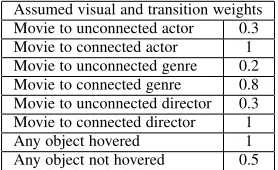
Assumed visual and transition weights
Movie to unconnected actor 0.3
Movie to connected actor 1
Movie to unconnected genre 0.2
Movie to connected genre 0.8
Movie to unconnected director 0.3
Movie to connected director 1
Any object hovered 1
[image:6.612.369.508.627.712.2]Any object not hovered 0.5
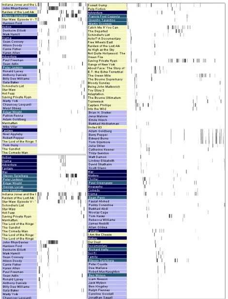
Fig. 4: PivotPaths visualization of IMDB data. Movies are displayed in the center of the screen, actors at the top, and directors and genres share the bottom space. Actors, directors, and genres associated to movies are connected through curves. Users can highlight objects and their connected neighbors by hovering over them.
Finally, as part of instrumentation, our system collected ap-plication screen shots, interactive events (e.g., hovering, zooming, panning), raw gaze samples captured at a rate of 120Hz, and visual elements with non-zero viewing scores computed at the same rate of 120Hz. For each viewed element we recorded the type (i.e., movie, actor, director, genre), its label, its gaze score (gs), its prediction score (ps), and the aggregated viewing score (vs). All recorded data was time stamped.
4
E
VALUATIONWe collected data from 9 subjects, each using our instrumented vi-sualization for approximately 50 minutes on a series of structured and unstructured tasks. We used this data data to test the validity and effectiveness of our approach in two ways.
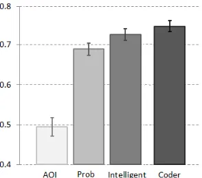
First, we compared the output of the intelligent algorithm to human annotation data. We found that data collected automatically was on average as similar to human annotations, as human annotations were similar to each other. Moreover, we conducted this analysis for all three viewed detection algorithms described in Sections 3.1.1 to 3.1.3 and found that the AOI algorithm performs
poorly compared to the other two, and that the predictive algorithm improves detection accuracy by about 5% (Figure 5).
Second, we demonstrate that our instrumentation method can provide relevant information and can be leveraged in novel and interesting ways. Specifically, we show both qualitatively and quantitatively that viewed objects detected by our instrumentation are closely correlated to the tasks we asked people to do, and that data collected automatically from many users can answer novel questions about how people use visualizations (Figures 6 and 7).
Third, we show quantitatively that the assumptions we made informally in the previous sections, about how people view our vi-sualization, hold. Specifically, as shown in Table 2, our users were significantly more likely to look at objects that were highlighted and connected to each other.
4.1 Study Design
Setup: We used the visualization and data described in Section 3, and an SMI RED-120Hz connected to a 17” monitor. Subjects were seated approximately 30′′away from the display.
them were male and three were female. Subjects were paid $10 for their participation.
Protocol: Subjects were first given a description of the study’s purpose and protocol. They were then introduced to our IMDB PivotPaths visualization and asked to perform a few training tasks to help them get accustomed with the visualization. This introductory part lasted on average 10 minutes. The main section of the study followed, involved multiple instances of four types of tasks, and lasted approximately 50 minutes.
Tasks: We asked subjects to complete four types of tasks. We aimed to balance structured tasks and unstructured tasks. To solve structured tasks, subjects had to consider a set of objects that was better defined and less variable than in unstructured tasks. This made it easier for us to test the degree to which our detection of viewed objects is aligned with the data required to complete the tasks. On the other hand, data collected for unstructured tasks may be better at informing designs of future analysis systems of such data. We limited the time we allowed subjects to spend on each task for two reasons: to manage the total duration of the study, and to make results comparable across time and users.
• Task1 (structured):Finding four commonalities between pairs of movies. The tasks were limited at three minutes each, and subjects solved the following four instances of this task: (a) Goodfellas and Raging Bull; (b) Raiders of the Lost Ark and Indiana Jones and the Last Crusade; (c) Invictus and Million Dollar Baby; (d) Inception and The Dark Knight Rises.
• Task2 (structured): Ranking collaborations between a director and three actors (2 minutes). Subjects completed four task instances centered around the following directors: (a) Ang Lee; (b) Tim Burton; (c) James Cameron; (d) David Fincher.
• Task3 (semi-structured): Given three movies, subjects were asked to recommend a fourth (5 minutes). Subjects solved three such tasks: (a) Catch Me If You Can, E.T. the Extra-Terrestrial, and Captain Phillips; (b) To Kill a Mockingbird, The Big Country, and Ben-Hur; (c) Inglou-rious Basterds, The Avengers, and Django Unchained.
• Task4 (unstructured): Given a brief and incomplete description of the “Brat Pack”, a group of young actors popular in the 80’s, subjects were asked to find additional members and movies they acted in. Subjects solved one such task, in approximately 5 minutes.
4.2 Results
4.2.1 Data collected automatically is similar to that of hu-man annotators
We tested whether the outputs of the three algorithms described in Sections 3.1.1 to 3.1.3 (AOI, probabilistic, and predictive) are comparable to annotation data obtained from human coders who inspected screen-captures with overlaid gaze samples and manually recorded what subjects looked at. As shown in Figure 5, we found that the overlap between human annotations and the predictive algorithm’ s output is similar to the overlap within the set of human annotations, and that the predictive algorithm outperforms the other two.
Specifically, we enlisted the help of five coders and asked them to annotate eye-tracking data corresponding to one task of approximately three minutes, for each of six subjects. The task was the same for all coders - task 1b. The six subjects
were selected randomly and were the same for all five coders. Coders spent approximately one hour per subject and six hours in total completing their annotation. This long duration meant it was unfortunately not feasible to code data from more users or more tasks than we did. Four coders completed all six assigned annotation tasks, while one was able to annotate the data of only three subjects.
Coders used an application that allowed them to browse through screen captures of a users’ activity with overlaid gaze coordinates. We asked coders to advance through the videos in 100ms time-steps, determine what visual objects their assigned subjects were viewing, and record those objects along with the start and end time of their viewing. If unsure which of multiple objects was viewed, coders were allowed to record all of them.
We transformed each coder’s annotation for each subject into temporal vectors with 100ms resolution. These vectors contained at each position one or several objects that were likely viewed by the subject during the 100ms time-step corresponding to that position. We then created similar representations from our automatically collected data. Finally, we defined a similarity measure between two such vectors as the percentage of temporally aligned cells from each vector that were equal. Equality between vector cells was defined as a non-empty intersection between their contents.
For each algorithm, we computed the similarity of its output for each subject’s data to all available human annotations of the same data. This yielded 4 coders × 6 subjects + 1 coder ×
3 subject = 27 similarities per algorithm. We averaged these similarities and plotted them as the first three bars in Figure 5. Then, we compared each coder’s annotation of a subject’s data to all other available annotations of the same data. Since we had five annotations for three subjects, yielding 3 subjects×10 annotation pairs = 30 similarities, and four annotations for the remaining three subjects, yielding 3 subjects × 6 annotation pairs = 18 similarities, this process resulted in a total of 48 similarities, which we averaged and plotted as the last bar of Figure 5.
The data we collected allowed us to perform this analysis for all three algorithms described in Section 3.1. Specifically, if we only consider gaze scoresgsthat are equal to one (Section 3.1.1) and no predictive component, we essentially have the output of the AOI algorithm. If we limit the analysis togsscores alone, without the prediction component described in Section 3.1.3, we have the output of the probabilistic approach described in Section 3.1.2.
4.2.2 Data collected automatically is relevant and useful
We used two visual representations and analyses to show that data collected automatically is tightly correlated with the tasks that users had to do. We chose this evaluation for two reasons. First, it provides evidence that the automatic instrumentation approach can be used to solve the inverse problem: an observer or analyst who is unfamiliar with a subject’s intentions can determine what these are by looking at the subject’s visual interest in particular data.
Fig. 5: Comparison between automated and manual viewed object detection. The first three bars show the overlap between the outputs of the three algorithms described in Section 3.1 and annotation results of human coders. The last bar shows the overlap within the set of human annotations. Values correspond to aver-ages over multiple tasks, multiple subject data sets, and multiple annotators, and are computed as described in Section 4.2.1. Error bars extend by one standard error.
First, we created heatmap representations from our collected data (Figure 6) to illustrate qualitatively the strong connection between the tasks our subjects performed and the data we collected. We listed viewed objects vertically, discretized viewing scores by aver-aging them over 500msintervals, and arranged them horizontally. Thus, time is shown horizontally, viewed objects vertically, and intensity of heatmap cells indicate the degree to which an object was viewed at a given moment in time. The viewed objects listed vertically were colored based on their type (movie, actor, director, genre) and could be sorted by either first time they were viewed, amount of viewing activity, or type.
Figure 6, left, shows the data collected from a subject per-forming task 1b: finding commonalities between two Indiana Jones movies. The upper heatmap is ordered by the amount of visual attention that the subject dedicated to each element in the visualization. We notice that elements at the top of the heatmap are tightly connected to the subjects’ task. In the bottom panel, viewed items are ordered by category (genre, director, movie, actor). We notice a clear temporal pattern: the movies involved directly in the task were viewed throughout the analysis, actors were considered early on, followed by genres, then directors, and ultimately a quick scan of other movies. We observed this pattern for most subjects and believe it was caused by the ordering used in the task’s phrasing: we asked subjects to determine actors, genres, and directors that were common between the two movies.
Figure 6, right, shows a subject’s results for one of the instances of task 3, which was significantly less structured than task 1 (see Section 4.1). This heatmap was sorted by the first time each object was viewed and shows how subjects were moving through different aspects of the analysis. Heatmaps associated to these task types typically showed a wider range of viewed objects, as indicated by the heatmap’s greater height. We attribute this pattern to the more exploratory nature of the task.
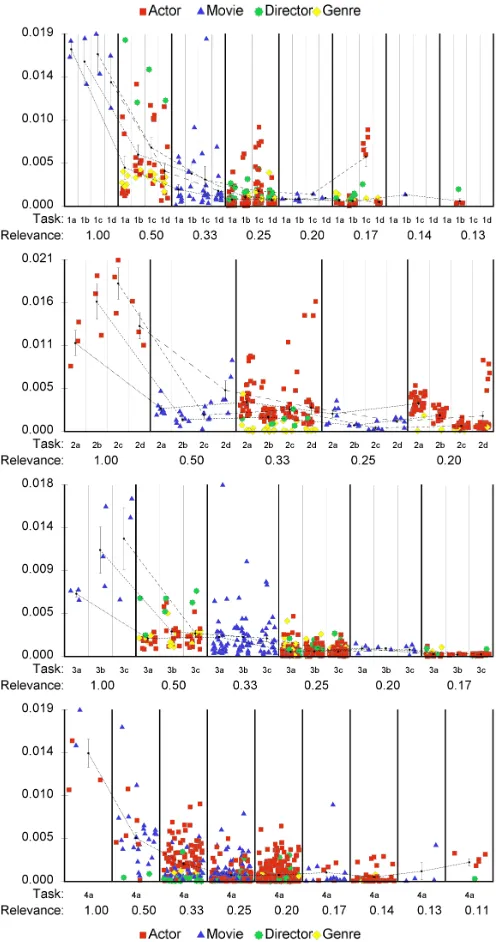
Second , we formalized the relevance of each visual item to a particular task and plot this relevance against the amount of interest that each item attracted, as shown in Figure 7. These plots quantify the degree to which tasks determine users’ interest in visual items, and demonstrates that our instrumentation captures
relevant data.
[image:9.612.101.248.42.172.2]We formalized the relevance of a visual item to a task as Relevance = 1/(1+d), whered is the shortest graph distance between that item and items mentioned directly in the task de-scription. To exemplify, the relevance of Goodfellas and Ranging Bull to task 1a is 1 as they are the focus of the task, that of Martin Scorsese is 1/2 because he directed both movies, while that of other movies directed by Scorsese is 1/3. This definition is not fully accurate as items might be relevant to a task even though they are not directly mentioned in the description. For instance, items that eventually constitute a user’s answer will elicit more attention. Moreover, this definition is particular to the visualization we instrumented.
Figure 7 facilitates several insights. First, even though many items were shown to subjects during their tasks, only very few were viewed for significant periods of time, and many were not viewed at all. Second, the types of data that users focus on correlates with the particularities of each task. For example, task 3 involved movie recommendations and Figure 7 illustrates that genres and directors were viewed significantly more than in task 4, which involved determining the identity of a group of actors and seemed to drive users to mostly focus their attention on actors.
4.2.3 Assumptions about viewing transition patterns hold
We performed a qunatitative analysis of our subjects’ viewing-transition patterns, using the data we collected during our study, and found that the informal assumptions we made in Section 3.1.3 were correct: our users showed strong preferences to view objects that were highlighted or connected to previously viewed objects. The last three columns in Table 2 compare the probability with which our users viewed one object category after another (e.g., viewed a highlighted actor after a movie) as computed from data we collected, to a null hypothesis in which users pick next items to view at random. The quantitative results show for instance that after viewing a movie, our users were four times more likely to look at an actor that was highlighted (Ratio=4.081), and eleven times more likely to look at an actor that was both highlighted and connected to the previously viewed movie (Ratio=11.484), than if users were viewing items at random.
To reach these results, we first discarded the prediction com-ponent from the data we collected, since it represents exactly the assumption we seek to evaluate. We then counted direct viewing transitions between all types of objects (sources) to all other types of objects (targets) and divided them into categories based on whether targets were highlighted, connected to the sources, or both (Table 2). For example, after looking at a movie title, our users looked at an actor that was unconnected to that movie and unhighlighted 793 times and at an actor that was connect to the movie and highlighted 616 times. Since in our visualization connections existed only between movies and actors, genres, and directors, transitioning to a connected or highlighted and connected target was only possible when transitioning to and from movies.
These counts were translated into observed transition probabil-ities by normalizing them by the total number of transitions from each type of source to each type of category. For example , our users transitioned in total 1784 times from a movie to an actor, of which 147 transitions were from a movie to a highlighted actor, yielding an observed transition probability of 147/1784=0.082.
Movie to
No. of transitions
Observed trans. prob.
Unbiased trans. prob.
Ratio Observed Unbiased
Actor
- 793 0.445 0.898 0.495
H 147 0.082 0.02 4.081
C 228 0.128 0.052 2.473
CH 616 0.345 0.03 11.484
Movie - 5727 0.761 0.899 0.846
H 1798 0.239 0.101 2.376
Director
- 304 0.537 0.887 0.606
H 37 0.065 0.021 3.088
C 51 0.09 0.055 1.647
CH 174 0.307 0.038 8.176
Genre
- 193 0.33 0.792 0.417
H 40 0.068 0.033 2.045
C 69 0.118 0.102 1.159
CH 282 0.483 0.072 6.693
Actor to
No. of transitions
Observed trans. prob.
Unbiased trans. prob.
Ratio Observed Unbiased
Actor - 4711 0.685 0.962 0.713
H 2164 0.315 0.038 8.207
Movie
- 839 0.469 0.82 0.572
H 213 0.119 0.058 2.046
C 386 0.216 0.076 2.843
CH 352 0.197 0.046 4.284
Director - 68 0.701 0.959 0.731
H 29 0.299 0.041 7.271
Genre - 43 0.524 0.931 0.563
H 39 0.476 0.069 6.918
Director to
No. of transitions
Observed trans. prob.
Unbiased trans. prob.
Ratio Observed Unbiased
Actor - 71 0.747 0.958 0.78
H 24 0.253 0.042 5.964
Movie
- 271 0.494 0.792 0.623
H 55 0.1 0.04 2.478
C 130 0.237 0.108 2.198
CH 93 0.169 0.06 2.841
Director - 384 0.706 0.93 0.759
H 160 0.294 0.07 4.216
Genre - 256 0.522 0.899 0.581
H 234 0.478 0.101 4.708
Genre to
No. of transitions
Observed trans. prob.
Unbiased trans. prob.
Ratio Observed Unbiased
Actor - 61 0.656 0.9791 0.67
H 32 0.344 0.021 16.47
Movie
- 229 0.118 0.261 0.453
H 46 0.024 0.008 3.001
C 172 0.089 0.093 0.956
CH 138 0.071 0.013 5.288
Director - 282 0.591 0.973 0.608
H 195 0.409 0.027 15.174
[image:11.612.313.561.42.513.2]Genre H- 348526 0.3980.602 0.9430.057 10.6270.422
[image:11.612.57.291.72.581.2]TABLE 2: Transitions from a source object to a target object, divided by: (i) type of source and target; (ii) whether the target was highlighted (H); (iii) whether the target was highlighted and connected to the source (HC); (iv) and whether source and target were neither highlighted nor connected. Columns show: (i) the number of direct transitions for the source/target combination; (ii) the observed transition probability from the source to that target; (iii) the (unbiased) probability of transition between source and target if all elements had equal probability to be viewed; (iv) the ratio between observed and unbiased transition probabilities.
Fig. 7: Users’ interest in data objects, in relation to each objects’ relevance to a task, for twelve tasks of four types. Each individual task is plotted in its type’s corresponding chart as a subdivision across multiple relevance categories. Relevance was computed as described in Section 4.2.2, and plotted for all objects that were visible to subjects during each task. The average interest in objects with the same task relevance are linked by separate polylines for each individual task; errors bars extend from the averages by one standard error.
Thus, observed transitions should be compared to the default case which assumes that users treat all visual objects equally. Assume the following simplified case: a movie is connected to two of ten actors shown in a visualization. We observe that of ten transitions from that movie to one of the actors, five were to a connected actor, while five were to unconnected actors. The two observed probabilities, to connected and unconnected actors, would in this case be equal at 5/10=0.5. However, if there was no transitioning preference, the probability of transitioning to any actor would be equal to 0.1, that of transitioning to a connected actor 0.2, while that of transitioning to an unconnected actor 0.8. Thus, our observed transition probability from a movie to a connected actor is 0.5/0.2=2.5 times higher than the default, unbiased probability, while our observed transition from a movie to an unconnected actor is a fraction (0.5/0.8=0.625) of the unbiased one.
To compute unbiased probabilities, every time we counted a transition from a source to a target, we also counted all target options available to a user at that point, given the state and structure of the visualization at the time of transition. Reverting to our simplified example, for each of our ten observed transitions we would count two possible transitions to connected actors and eight possible transitions to unconnected actors, ending up with 20 counts for connected actors, and 80 counts for unconnected actors. These numbers allow us to compute the two unbiased probabilities as 20/(20+80)and 80/(20+80).
5
D
ISCUSSION 5.1 BenefitsIt took each of our coders approximately six hours to produce a detailed and accurate coding of just eighteen minutes of user data (6 subjects × 3 minutes). This illustrates the importance of moving beyond interpreting eye-tracking in stimulus space. The instrumentation we described and evaluated makes it feasible to analyze eye-tracking data from many subjects, using highly interactive content, for long analysis sessions. Such analyses can be done immediately after or even as the data is collected since no manual annotation of the data is required.
Moreover, the collected data has semantic meaning that is tied to the underlying data of the visualization and is thus amenable to a much richer set of visual and computational analyses than tradi-tional eye-tracking data. Such analyses, which we exemplified in Sections 4.2.2 and 4.2.3 , focus on data and concepts, and are thus significantly different from current eye-tracking analyses, which generally are aimed at understanding low-level visual perception in static visualizations.
Our work provides a quantitative framework that can be used to explore questions related to how users perceive visualizations in general, how domain experts look at particular types of data, and how analysts use visualization to search for relevant data and aggregate them into hypotheses. Currently, visualization re-searchers often have to rely solely on discussions with domain experts, think aloud studies, and recordings of user activity, all of which provide only qualitative data and often require additional coding and interpretation.
5.2 Applications
As described above, our approach can be useful in understanding how users forage for, integrate, and hypothesize about data using
complex, interactive visualization systems. For example, visual analytics applications could be instrumented to facilitate the ex-ploration of domain expert workflows, of how expertise influences data search and analysis patterns, and of visual strategies and data associated with successful hypothesis generation and testing. Similarly, the instrumentation of visual learning environments could lead to insight into how students learn and what makes some learners more effective than others. Given the proliferation of education through visual, interactive environments, particularly as part of massive MOOC instruction, this could have significant impact.
In both aforementioned cases, the data can also explain how visualizations support analysis, discovery, and learning, and how they may be changed to make them more efficient. For example, given a particular domain, we could quantify which data best answers which questions, what types of data are often used together, and how visual widgets are viewed in an analysis process. Results could then be used to optimize specific visualizations systems or generic visualization methods. Section 4 exemplifies quantitative and qualitative analyses that are possible using our approach.
Viewing data collected automatically during a user’s session could also be used more directly to support analytic workflows. For example, the data could be transformed automatically into summaries that capture the user’s activity during a day, week, or month. Such summaries could be used to refresh the user’s mem-ory at a later time, communicate progress to peers or supervisors, and provide useful hints to other users or analysts exploring similar questions in similar data-sets.
Moreover, detecting viewed objects online opens up two specific opportunities. First, analyzing eye-tracking data in real-time could be used in teaching. By instrumenting learning envi-ronments, we could allow instructors to track students’ progress in lab assignments in real-time, to detect students that are not tending to elements crucial for solving or understanding the assigned problems, and to provide help proactively. Second, it would allow us to create a new generation of gaze-contingent visualizations that can detect in real-time data that is of particular interest to a user and make recommendations of unexplored data with similar attributes. The ever lower cost of eye-trackers, currently under $150, makes it conceivable that eye-trackers may be included in regular work stations, rendering our suggested new applications as potentially impactful.
5.3 Limitations
Our approach is restricted to visualizations with open source code and cannot be used to automate the full spectrum of current eye-tracking studies (e.g., analysis of real imagery or of commercial systems). This problem is to some degree inherent to any software or hardware instrumentation: whether one wishes to capture an application’s interaction data, a website’s activity, or a network’s throughput, one needs privileged access to those systems. Thus, like most instrumentations, our approach is intended primarily for creators or owners of data visualizations who wish to understand how their visualizations are used, and to discover changes that could make their visualizations more efficient. Moreover, this limi-tation is offset by new analysis and interaction opportunities which our approach enables, a few of which we discussed previously.
an overhead. This is also a general instrumentation problem and should be solved on a case by case basis, by considering of the tradeoff between the overhead of instrumenting a specific system and the benefits of collecting data from it. For example, if the development of a visual analytics system takes a year from re-quirements elicitation to final implementation, and instrumenting it would allow developers to gain significant insight into how the system is used, then spending an extra week to instrument the rendering code may seem warranted. Our future plans include bundling the predictive algorithm into an instrumentation library (Section 5.6) to reduce the cost of instrumenting visualizations.
Finally, picking the right parameters to our predictive algo-rithm may be difficult for some visualizations, given that a solid understanding of how users parse and interpret visualizations does not yet exist. To address this, in Section 4.2.3 we give a methodology to quantify transition and viewing probabilities from real data collected from users. Such computations could be performed during a pilot study, to reveal usage patterns in a par-ticular visualization. Furthermore, since we believe visualizations are rarely used in a random fashion and that specific tasks and visual outputs elicit certain gaze patterns, we think further research could lead to a more general understanding of the probabilities our algorithm relies on. More importantly, our framework facilitates exactly this type of unexplored questions in ways previously not possible, as exemplified by the analyses in Section 4.
5.4 Performance gains by using a predictive approach
An important contribution was to show that by leveraging a predictive model of how users view data in a visualization we can detect objects more accurately than by just relating gazes to visual object geometry. While in our particular example the gain was relatively small (5%), we think that benefits are highly dependent on the type of visualizations that are instrumented, and that some visualizations will benefit significantly more from the predictive approach.
This belief is supported by the results shown in Table 2, which reveal very strong biases in how people use visualizations (e.g., subjects were up to 11 times more likely to view highlighted items connected to previously viewed items, than to view random other items). We believe this to be generalizable to many visualizations, especially those that show large, heterogeneous data, and those that are intended for in-depth, focused analyses. The first aspect means that the same data are likely to be used differently based on context and task. The second aspect means that tasks can significantly constrain what data is viewed.
The degree to which such viewing patterns can and need to be leveraged predictively depends on the particularities of each visualization. For example, in our particular case study, the different data categories (i.e., movies, directors, actors, genres) were spatially separated in different panels. As such, if a gaze landed between multiple data objects, these were generally of the same type. This means that our algorithm never got the chance to use object category as a discriminator. Instead, in a traditional node link diagram for example, multiple definable categories of nodes share the same space, and are distinguishable by specific visual attributes or semantic meaning (e.g., proteins in a protein interaction network can be kinases, receptors, etc.). In such a case, an algorithm could use knowledge that a user is currently scanning for, or generally more interested in, a particular type of node, to distinguish between the viewing of nodes that are placed next to each other but are from different categories.
More generally, a visualization will benefit more from our predictive approach if heterogeneous content is cluttered and shares the same space, and the visualization provides visual and semantic cues that allow users to select subsets of data that are relevant to a particular task or analysis. Such visualizations are fairly commonly used in real, complex visual analytic applica-tions. Instead, if the visual content is sparse and well separated, then computing gaze scores alone would be sufficient and our algorithm’s predictive component would not create any benefit.
5.5 Evaluating viewed object detection
The above mentioned variability in accuracy makes it hard to assess the real impact of the predictive method. Moreover, compar-ing the output of the predictive algorithm to annotations of human coders is questionable since, if coders look primarily at momentary gaze positions, rather than trying to understand what users aim to do more broadly, then their annotation may be closer to our our simpler, probabilistic detection. This latter problem raises an issue about whether human coders can provide a robust ground truth for evaluating techniques such as ours, and whether such ground truths could be improved if eye-tracking data was collected in conjunction with a think-aloud protocol.
First, we note that we see the quantitative evaluation described in Section 4 as an evaluation against the state-of-the-art rather than against a ground truth. In other words, we don’t claim that our method produces results that are accurate with respect to what people actually looked at. Instead, we claim that our method allows us to analyze the data in the same way a human could, only much faster.
Second, we believe that striving towards a reliable ground truth is slightly misguided in the context of evaluating eye-tracking instrumentation. People often view elements even without con-sciously realizing it, since vision is by-and-large a subconscious process [3]. People also are able to register multiple objects in a fixated region, while not fixating any one object specifically. For example, while reading people often skip short words or syllables, while still registering that they are there. Moreover, for specific tasks, people may think about multiple objects as single data units of analysis. For example, a user of a graph visualization might think in terms of nodes for some tasks (e.g., are two nodes connected?) but may reason in terms of clusters of nodes or cliques for other tasks (e.g., what is the largest clique in the graph?). In the latter case users may fixate at the center of a node cluster to assess the properties of the cluster as a whole, rather than fixate on individual nodes. Finally, people also occasionally stare at visual objects while in fact thinking of something else [3]. These issues lead to interesting questions about whether we track what subjects look at or what they see.
given by Ogolla who showed that concurrent think-aloud protocols change visual patterns, especially for exploratory tasks [41].
Finally, the evaluation described in Section 4.2.2 implements in fact an evaluation against a ground truth that is loosely defined by the tasks subjects had to do. These tasks, especially the structured ones, dictated what users had to look at in order to solve them, and the two visual representations in Figures 6 and Figure 7 indicate how close our automatically collected data comes to that ground truth. Such ground truths are somewhat approximate and not sufficiently detailed, but can nevertheless show that data collected automatically is relevant.
5.6 Future Work
We hypothesize that there is a set of general principles about how people take in visual and data content that are valid across visualizations. For example, most visualizations have a mechanism for highlighting specific elements, either through interaction or through queries, and we showed that this highlighting matters in how people view elements. Second, while we studied connected elements in the context of a node-link like diagram, establishing a visual connection between elements is also employed in brushing and linking interactions or the use of leader lines. We think our finding that users view connected elements together also applies to these more general cases. Third, most data featured in visual-ization can be divided into semantic groups (e.g., actors, movies, directors; protein kinases, protein receptors; conference papers, journal papers) and we hypothesize that viewing transitions be-tween and within such categories are also not random. Finally, we showed that in our particular case study, users identified data that is highly connected to their task and then shifted their attention repeatedly and almost exclusively within that data group. Again, we believe this is a behavior that is generalizable. Demonstrating these generalities and exploring other patterns is beyond the scope of this paper but the framework we proposed allows us to easily explore and quantify such patterns in other visualizations. This would both deepen our understanding of how visualizations are used and provide guidelines for choosing appropriate inputs to our algorithms.
More work is also needed to understand the impact of different parameters involved in viewed object detection. For example, how far away from an item can a user fixate and still be considered to be viewing the item? The parameter that captures this in our algorithm isR, and, while we use a constantRfor all items, this is unlikely the best approach. Based on qualitative observations in the data we collected, and knowledge of the interplay between peripheral vision and the fovea [42], we believe users fixate close to items if they are surrounded by clutter, but exhibit significantly more variability if items are isolated. Thus, we hypothesize thatR
should adjust itself dynamically based on the clutter of the region that a user is fixating. A further question is whetherRshould be changed based on the visibility or discriminating features of an item: can subjects fixate farther and still perceive an item if that item is large enough?
Additional work is also needed to understand how to and whether we can detect visual objects other than nodes or labels, such as for instance polylines in a parallel coordinate plot, con-tours in a group or set visualization, or cells in a heatmap. It is unclear how to compute a gaze score (gs) for such objects since there is no research to describe how people fixate them.
Finally, to reduce the overhead of instrumentation, our future plans include making the predictive algorithm available as an
instrumentation library. A developer would link this library to the visualization and maintain a correspondence between what is shown on the screen at any given time and visual objects registered with the library. Thus, when a new object is added to or removed from the screen, or when its position or shape changed, these changes would need to be registered with the library. Interestingly, this workflow would integrate well with the add-remove-update pattern typical of D3. Additionally, developers would create classes of objects, for instance based on data semantics (e.g., kinases, movies, actors) or visual aspect (e.g., highlighted, glyphs of a certain kind), and specify transitions probabilities between them. The library would implement the algorithms described here and provide in real time a list of visual items that a user is viewing.
6
C
ONCLUSIONIn visualizations that are open to instrumentation, gaze informa-tion provided by an eye-tracker can be used to automatically detect what visual objects users are likely to be viewing. Such detection can provide results that are almost as accurate as annotations created by human coders, provided that detection is done “intelli-gently”, by using gazes together with a prediction of which objects are likely to be viewed at a given time. Data collected in this way is highly granular and has semantic content because it is linked to the data underlying the visualization. For this reason, and because it does not require any human pre-processing, object viewing data can be collected and analyzed efficiently for many subjects, using interactive visualizations, for long analytic session, and could be used in studies that explore how analysts hypothesize about data using complex visual analytics systems.
R
EFERENCES[1] C. Ware and H. H. Mikaelian, “An evaluation of an eye tracker as a
device for computer input2,”ACM SIGCHI Bulletin, vol. 18, no. 4, pp. 183–188, 1987.
[2] R. J. Jacob, “The use of eye movements in human-computer interaction
techniques: what you look at is what you get,”ACM Transactions on
Information Systems (TOIS), vol. 9, no. 2, pp. 152–169, 1991.
[3] A. T. Duchowski, Eye tracking methodology: Theory and practice.
Springer, 2007, vol. 373.
[4] K. Rayner, “Eye movements and cognitive processes in reading, visual search, and scene perception,”Studies in Visual Information Processing, vol. 6, pp. 3–22, 1995.
[5] S. Stellmach, L. Nacke, and R. Dachselt, “3d attentional maps: aggre-gated gaze visualizations in three-dimensional virtual environments,” in Proceedings of the international conference on advanced visual interfaces. ACM, 2010, pp. 345–348.
[6] F. Papenmeier and M. Huff, “DynAOI: A tool for matching
eye-movement data with dynamic areas of interest in animations and movies,” Behavior Research Methods, vol. 42, no. 1, pp. 179–187, 2010. [7] D. D. Salvucci, “Inferring intent in eye-based interfaces: tracing eye
movements with process models,” inProceedings of the SIGCHI
con-ference on Human Factors in Computing Systems. ACM, 1999, pp. 254–261.
[8] D. D. Salvucci and J. R. Anderson, “Intelligent gaze-added interfaces,” in Proceedings of the SIGCHI conference on Human factors in computing systems. ACM, 2000, pp. 273–280.
[9] L. Sesma, A. Villanueva, and R. Cabeza, “Evaluation of pupil center-eye corner vector for gaze estimation using a web cam,” inProceedings of the symposium on eye tracking research and applications. ACM, 2012, pp. 217–220.
[10] K. Guo, H. Shawet al., “Perceiving facial expression from varying face orientations: an eye-tracking study,” 2014.
[11] J. R. Shasteen, N. J. Sasson, and A. E. Pinkham, “Eye tracking the face in the crowd task: why are angry faces found more quickly?”PloS one, vol. 9, no. 4, p. e93914, 2014.