Surplus Identification with Non Linear Returns ESRI WP522 December 2015

ESRI working papers represent un-refereed work-in-progress by researchers who are solely responsible for the content and any views expressed therein. Any comments on these papers will be welcome and should be sent to the author(s) by email. Papers may be downloaded for personal use only.

Surplus Identification with Non-Linear Returns

Peter D. Lunn* and Jason J. Somerville†

Abstract: We present evidence from two experiments designed to quantify the impact of cognitive constraints on consumers' ability to identify surpluses. Participants made repeated forced-choice decisions about whether products conferred surpluses, comparing one or two plainly perceptible attributes against displayed prices. Returns to attributes varied in linearity, scale and relative weight. Despite the apparent simplicity of this task, in which participants were incentivised and able to attend fully to all relevant information, surplus identification was surprisingly imprecise and subject to systematic bias. Performance was unaffected by monotonic non-linearities in returns, but non-monotonic non-linearities reduced the likelihood of detecting a surplus. Regardless of the shape of returns, learning was minimal and largely confined to initial exposures. Although product value was objectively determined, participants exhibited biases previously observed in subjective discrete choice, suggesting common cognitive mechanisms. These findings have implications for consumer choice models and for ongoing attempts to account for cognitive constraints in applied microeconomic contexts.

*Corresponding Author: [email protected]

† Department of Economics, Cornell University.

Keyword(s): Surplus Identification, capacity constraints, bias and precision, S-ID Task

JEL Codes: D11, D12, D81, D83

Acknowledgements: These experiments were conducted as part of PRICE Lab, a research programme funded by four economic regulators in Ireland: the Central Bank of Ireland, Commission for Energy Regulation, Competition and Consumer Protection Commission and ComReg. The authors are especially grateful to Mark Bohacek for assistance with the experimental environment and design, to Stephen Lea, George Loewenstein, Féidhlim McGowan and Ted O'Donoghue for illuminating discussions and comments on drafts, and to audiences at the Economic and Social Research Institute, Network for Integrated Behavioural Sciences and Trinity College Dublin for feedback.

1

Introduction

Benefit accrues to economic agents through the process of exchange when what is acquired is worth

more than what is given up. A prerequisite for making gains from trade, therefore, is that agents

can accurately identify surpluses. This paper presents evidence that cognitive limitations disrupt

surplus identification, even when agents attend fully to a small volume of complete information. The

findings have implications for consumer choice models that aim to incorporate cognitive constraints

and the response of firms to such constraints.

To spot surpluses agents must integrate information about product attributes and prices.

Re-turns to different attributes and combinations of attributes may vary in scale and linearity.

Further-more, in a dynamic economy, prices, attributes and preferences evolve. Learning new associations

between them is an ongoing process for agents seeking to maximise utility; a process that is subject

to at least occasional error. Most of us have goods tucked away at home that did not live up

to our assessment when we bought them, as well as cherished possessions that we value far more

than originally anticipated. Doubtless such outcomes are, in part, due to stochastic variation in

unobservable product quality, but they may also be caused by failure to integrate observable

infor-mation accurately when deciding to purchase, i.e., to imprecise identification of surpluses. Thus,

the human ability to integrate non-linear and, often, novel attribute information is fundamental to

economic exchange and market efficiency. It is this ability that we examine experimentally.

Empirical assessment of how accurately people identify surpluses is, of course, hampered by the

subjective and unobservable nature of preferences. Previous investigations have mainly focused on

markets where relative surpluses can be (nearly) objectively defined, for example where goods are

(effectively) homogeneous (Grubb, 2009; Wilson and Waddams Price, 2010; Choi et al., 2010). The

assumption is that where consumers opt to pay more for essentially the same product they are failing

to identify surpluses accurately. The evidence, reviewed briefly below, suggests that consumers in

some markets fail to identify the highest surpluses, with mixed evidence regarding learning. Such

findings are generating an increasingly rich theoretical literature, with contrasting approaches to

the formalisation of cognitive constraints within models of consumer decision-making (Woodford,

2014), discrete choice (Matejka and McKay, 2015) and, increasingly, industrial organisation (Grubb,

2015).

adapted from the study of perceptual detection, keeping product attributes and associated returns

under complete experimental control. As described in detail below, we incentivise participants

to identify objectively defined surpluses based on a price and just one or two directly observable

product attributes. The method measures the magnitude of surplus required for reliable detection

when returns to attributes differ in linearity, scale and relative weight. The results reveal how the

accuracy of consumers’ surplus detection varies as a function of the shape of attribute returns. This

variation in accuracy is illuminating with regard to the concept of a “complex product”, which is

extensively used but rarely defined.

Our experimental results suggest that descriptively accurate choice models might focus on

im-precision in the integration of information when consumers must map incommensurate internal

scales to compare attributes and prices. We show that this imprecision is large and varies

sys-tematically with the shape of attribute returns. When people map attribute magnitudes to prices

they are able to detect a surplus reliably only when it corresponds to a substantial proportion of

the price or attribute range. The experiments reveal that surplus detection is largely unaffected

by whether returns are linear or non-linear, provided they are monotonic, but that it deteriorates

when returns are non-monotonic. Moreover, despite considerable exposure to the product and

re-peated feedback, decisions are subject to persistent biases, with only a modest role for learning.

We conclude that inaccuracy of surplus identification on this scale is likely to be an important

determinant of consumer outcomes in different product markets, with associated implications for

microeconomic models. The magnitude of the errors we uncover is consistent with Luce’s (1959)

view that decision-making is essentially a process of probabilistic choice.

The paper is organised as follows. Section 2 briefly reviews evidence on the ability of consumers

to identify surpluses, together with relevant theoretical developments. Section 3 describes the

“Surplus Identification” (S-ID) Task. Section 4 describes Experiment 1, which investigated surplus

identification for single-attribute products with varying degrees of diminishing returns. Section 5

presents Experiment 2, which increased the complexity of the attribute-price relationship via a

sec-ond attribute and non-monotonic associations. Section 6 explores additional hypotheses regarding

2

Literature review: Limits to Surplus Identification

2.1 Empirical Evidence

A growing empirical literature documents how consumers, in at least some markets, miss out on

surpluses. Apparent “mistakes” can be identified without the need to make strong assumptions

about preferences where offerings are (effectively) homogeneous and so the maximisation of

con-sumer surplus reduces to a process of cost minimisation, assuming positive marginal utility of

money. For instance, substantial numbers of mobile phone consumers fail to choose the lowest cost

tariff for their personal pattern of usage from a limited number of non-linear price plans (Grubb,

2009; Lambrecht and Skiera, 2006), probably because of overconfidence and inattention (Grubb

and Osborne, 2015). Similar evidence has been obtained for two- and three-part tariffs in domestic

electricity markets by Wilson and Waddams Price (2010), who conclude that “many of the choices

are consistent with genuine decision error or inattention” (p.665). Consumers in these studies faced

non-linear price structures. Some evidence suggests that non-linear returns to attributes may be

difficult for consumers to assess, including non-linear measures of fuel efficiency in the car market

(Larrick and Soll, 2008) and returns to compound interest in financial services markets (Lusardi

and Mitchell, 2011).

Other evidence suggests that consumers sometimes fail to assess surpluses accurately because

they overweight largely irrelevant but prominently advertised product attributes, or underweight

price components. This can be as simple as overweighting premium brands and, hence, failing to

benefit from cheaper generic medicines (Bronnenberg et al., 2015). In relation to indexed mutual

funds, laboratory experiments (Choi et al., 2010) and data on fund flows (Barber et al., 2005)

suggest overweighting of past performance information and underweighting of fees. This may have

implications for market structure since, despite the homogeneity of the good, price dispersion for

indexed funds rivals that for actively-managed ones (Hortacsu and Syverson, 2003). Grubb (2015)

reviews additional evidence for consumer errors when prices are multidimensional.

2.2 Constrained Capacity in Consumer Choice Models

Since at least Simon (1955), some microeconomic models have sought to incorporatebounded

ad-ditional capacity constraints to an otherwise standard utility maximisation model (Lipman, 1995).1

More recent models ofrational inattentionexploit information theory to recast economic agents as

input-processing vehicles subject to finite Shannon capacity limits (Sims, 1998, 2003; Sims et al.,

2010).2 Agents allocate limited attention optimally across information sources.3

Contrastingly, Woodford (2014) applies a capacity constraint to the processing of information

over time rather than across multiple sources, modelling the agent as an optimal sensor facing a

discrete choice, where the benefit of waiting to observe more signals trades off against the

prob-abilistic cost of an option becoming unavailable. Again, a fundamental limit is imposed on the

mutual information between the input state and an output signal, but the central trade-off to be

optimised differs. Because Woodford (2014) incorporates time, his model makes predictions about

decision response times that we test via the S-ID task.

Models of rational inattention provide generalisable explanations for stochastic errors, but little

guidance on the extent of inaccuracy or variation in errors across contexts. Other approaches

maintain the optimisation framework but introduce a non-optimal “behavioural” assumption to

explain why, in specific circumstances, surpluses may not be accurately identified. K˝oszegi and

Szeidl (2013) propose that utility is “focus weighted”, with greater weight placed on attributes

that differ most between available options. Bordalo et al. (2013) make the similar, but distinct,

assumption that additional weight is given to options with attributes that stand out relative to

other options. Implicit is a more general assumption about cognitive capacity, namely that there is

either too much immediate attribute information or too great a reliance on memory for attribute

weights. The result is context-specific calibration and, hence, non-optimal attribute weighting and

inaccurate surplus identification.

The above models represent advances in our understanding of how agents might miss out on

surpluses. Despite differences of approach, they possess important commonalities. Cognitive

ca-pacity is constrained with respect to the volume of relevant information that can be processed, or

attended to, simultaneously. However, the models make only limited predictions about the

mag-nitude and variability of errors. Yet the source of inaccuracies, their scale and variation across

1_{Alternative approaches dispense entirely with the concept of optimisation in favour of heuristics (see Gigerenzer}

and Selten (2002)). See also Harstad and Selten (2013) and Rabin (2013).

2_{While Shannon Entropy has been primary used to model information-processing costs in the rational inattention}

framework, more generalized cost functions exist (see Caplin and Dean (2013)).

3_{When each option is equally likely to be chosen ex ante, the probability of choosing an item reduces to the}

markets have further theoretical significance. Most obviously, small individual errors may imply

trivial deviations from optimal outcomes, but large errors could imply significant welfare losses.

Consumer errors have implications for industrial organisation too. An increasingly developed

the-oretical literature explores the implications when the potential for errors is endogenous both to the

extent of consumer search and to firms’ decisions to exploit opportunities to obfuscate quality or,

more commonly, price (Gabaix and Laibson, 2006; Carlin, 2009; Wilson and Waddams Price, 2010;

Ellison and Wolitzky, 2012; Grubb, 2015). While space does not permit a thorough treatment

here, two points are notable. First, there is empirical evidence of firm obfuscation (Ellison and

Ellison, 2009; Muir et al., 2013). Second, the precise source of consumer error can be important to

firms’ decisions to obfuscate, to equilibrium price dispersion and to the relationship between prices

and marginal costs (Gabaix and Laibson, 2006; Gaudeul and Sugden, 2012; Gabaix et al., 2015;

Spiegler, 2014).

2.3 Learning to Identify Surpluses

The view that preferences develop over time through mistakes and feedback forms the basis of

Plott’s (1996)discovered preferences hypothesis. Applied to surplus identification, it suggests that

consumer mistakes reduce with feedback and market experience as consumers learn what they like.

Evidence of consumers’ capacity for learning is mixed. Costly mistakes can lead consumers to

make better choices, for instance in local telephony and credit card markets (Miravete, 2003;

Agar-wal et al., 2005, 2008). However, in telecommunications and electricity markets consumer mistakes

have been shown to persist (Lambrecht and Skiera, 2006) and to repeat over multiple switches

(Wilson and Waddams Price, 2010). This mixed evidence may imply that different psychological

mechanisms are key to different instances where consumers misjudge surpluses. The nature of

feed-back may matter. A credit card customer who does not initially consider the possibility of incurring

a particular penalty, may factor this possibility in after a single application of the fee. In contrast,

if surpluses are misjudged in a market with multiple product attributes or price components, agents

may remain unaware of the missed surplus and, consequently, error prone.

Even given sufficient information and feedback, evidence from psychology suggests that the

potential for learning may ultimately be limited. Dating back to Miller (1956) and beyond, an

that require them to process, simultaneously, more than around four separate “chunks” of

infor-mation (Cowan, 2000). A substantial literature also investigates the ability to learn functional

relationships, typically by requiring individuals to predict outcomes based on the magnitudes of

multiple cues. Broadly speaking, simple monotonic associations are learned best, but performance

deteriorates as cues are added and non-linear functions become more complex (Busemeyer et al.,

1997).

3

The Surplus Identification (S-ID) Task

3.1 Conceptual framework

The empirical research described above highlights markets where consumers misjudge surpluses.

Models of consumer choice and industrial organisation have been amended to account for the implied

limits to cognitive capacity. Yet a richer understanding of the prevalence, magnitude, persistence

and cause of consumers’ failure to identify surpluses is required. The experiments described here

offer a fresh approach, which centres on obtaining full experimental control over the scale, linearity

and relative weight of product attributes. This section introduces the logic of the experimental

task.

The Surplus Identification (S-ID) Task is an experimental paradigm devised by Lunn and

Bo-hacek (2015). It measures consumers’ ability to integrate attribute information from first

princi-ples, beginning with simple products that possess a single clearly observable characteristic, then

increasing complexity in an experimentally controlled fashion. In this way, it permits the empirical

isolation of those aspects of the attribute-price relationship that have a negative impact consumers’

surplus identification, allowing controlled investigation of what truly constitutes a “complex”

prod-uct. This contrasts with previous approaches that test for consumer biases in specific markets.

Instead the task isolates cognitive limitations that are likely to generalise across markets.

The S-ID task blends techniques from studies of perception, psychophysics and experimental

economics. Participants are presented with novel, computer-generated products, consisting of one or

more attributes and a price tag. We refer to these products as “hyperproducts”, because they permit

complete experimental control over the attribute-price hyperspace. Our hyperproducts possess

participants, thereby minimising any influence of prior beliefs or preferences. The attributes consist

of standard perceptual stimuli, the relative magnitudes of which previous studies of perception have

shown can be discriminated with high accuracy. This is important, because we are interested in how

accurately consumers integrate information to gauge surplus, not how accurately they discriminate

perceptual magnitudes.

The S-ID task tests surplus identification via a two-alternative forced-choice (2AFC) task,

as routinely employed in studies of perceptual detection (Macmillan and Creelman, 2004). The

attribute-price relationship is set by the experimenters and participants are incentivised to learn

it from examples and practice with feedback. Prices, attribute magnitudes and, hence, surpluses,

then vary over a succession of trials. On each trial, the consumer judges the surplus to be either

positive or negative, responding via one of two buttons, then receiving feedback. The S-ID task

therefore simulates the process of encountering a new product, making repeated purchase decisions

and receiving feedback about the surplus gained (or lost). Thus, the task circumvents the problem

of unobservable preferences by incentivising participants to identify surpluses that are objectively

defined and expressed in monetary terms. With this level of experimental control, surplus can be

varied from trial to trial and a precise statistical estimate of the probability of detection obtained.

Moreover, because the data are collected as a time-series, the extent and speed of learning can be

observed.

The S-ID task borrows from experimental economics by offering a clear incentive to adopt the

preference function set by the experimenters. In the experiments described below, a tournament

incentive was used. The most accurate performers received a significant monetary reward. Hence,

each participant’s unambiguous incentive was to learn and to apply the objective function that

related attribute magnitudes to prices as quickly and accurately as possible.

Several properties of the S-ID task are important to note. First, it is not a valuation or

pricing task: participants do not generate estimates of value or price, but decide only whether a

surplus is present. This feature is by design. When consumers decide on purchases they do not

typically generate numeric assessments. Second, participants are not placed under time pressure

but complete the sequence of trials in their own time, generally taking longer on more difficult trials.

While it is an empirical question as to whether surplus identification might improve with longer

feel they need to. Third, the unambiguous incentive to adopt the predetermined attribute-price

relationship imposes preferences upon participants. We contend that this process mimics learning

to apply subjective preferences formed through experience of real products. As described below,

the data offer empirical support, since we observe biases in our data that parallel those observed

in subjective discrete choice experiments, implying common cognitive mechanisms.

Overall, we find that participants readily grasp the idea of the S-ID task and compete for

rewards. The level of experimental control over repeated decisions generates rich data and permits

analyses that are beyond what is typically possible in most consumer choice experiments.

3.2 Main Measures

The SI-D Task is able to distinguish between inaccuracy arising from bias and from imprecision.

To quantify these effects, we employ two concepts from psychophysics: the “point of subjective

equality” (PSE) and the “just noticeable difference” (JND). Both correspond to the parameters of

a logistic “psychometric function” fitted to the bivariate data, where the binary dependent variable

is whether the participant responded that the surplus was positive and the continuous exogenous

variable is the magnitude of the surplus. When the surplus is very high, participants always respond

that it is positive; when it is very low they always respond that it is negative. Intervening levels

produce probabilistic responses.

The PSE and JND correspond to the location and slope respectively of the best fitting

psycho-metric function. Figure 1 illustrates the PSE and JND for data from a participant in one condition

in our first experiment. The PSE estimates the surplus at which the participant responded with a

probability of 0.5. Thus, the negative PSE indicates overestimation of surplus; a positive PSE would

indicate underestimation. One JND is then the difference in surplus required for the probability

that the participant detected a positive (or negative, since the psychometric function is symmetric)

surplus to rise from 0.5 to 0.86, which equates to one standard deviation of the underlying logistic

distribution. For an unbiased subject, it estimates how much surplus is needed to identify the

We model the probability of responding “Yes” to a surplus by the standard logistic formula, 4

Pr(“Yes”) = exp(θ0+θ1Surplus(%)) 1 + exp(θ0+θ1Surplus(%))

. (1)

The estimated coefficients for this sample data are θb₀ = 0.77 and θb₁ = 9.50, giving a PSE of

b

θ0/θb₁ = −8.1% and a JND of π/(θb₁

√

3) = 19.1%. Hence this participant perceived zero surplus

when in fact there was a negative surplus of 8.1%. The JND indicates than the participant required

an increase in surplus equivalent to 19.1% of the price range to detect it with 86% reliability.

Figure 1: Sample data from experiment 1

The primary analyses measure changes in the PSE and JND by condition and over time.

Es-timating individual psychometric functions by participant and condition – as in equation (1) –

entails loss of statistical efficiency, so we instead estimate mixed effects logistic (MEL) models to

the complete data. Individuals are assumed to vary randomly in bias and precision, allowing for a

correlation between the two. Tests for changes by condition in the underlying fixed effects

param-eters constitute the main hypothesis tests of interest. Relative to an individual-level analysis, this

approach improves statistical power (Moscatelli et al., 2012).

4_{The use of a logistic is standard in psychophysics and micro-founded by models of rational inattention in situations}

4

Experiment I

The most simple test of surplus identification with non-linear returns involves a single-attribute

product with a monotonic, continuous relationship between attribute and price. Experiment 1

aimed to generate baseline measures of accuracy and learning when facing diminishing returns to

attributes of varying degrees.

4.1 Method

Consumers from the Dublin area (N=36) were recruited through a market research company,

bal-anced by gender (19 female), age (M=36.1; SD=12.8) and working status (61% employed). Each

received a e20 participation fee. Participants were informed that the most accurate performer in every ten would win a e50 shopping voucher. (In addition to the main sample of 36, another 26 participants completed a pilot experiment to test how accurately the product attributes could be

discriminated, as briefly described at the beginning of Section 4.2).

The three “hyperproducts” used were Golden Eggs, Victorian Lanterns and Mayan Pyramids

- products with intuitive value that participants would be highly unlikely to have valued or traded

previously. Each hyperproduct could vary on two attributes (see Figure 2).5 _{For the Golden Egg,}

overall size and the fineness of the surface texture (highest spatial frequency component) varied.

For the Victorian Lantern, the ratio of an inner blue flame to the overall flame and the number of

sparks emitted from the base varied. For the Mayan Pyramid, the width of the staircase and the

mouldiness of the bricks varied. On any one experimental run, however, participants attended to

only a single attribute, which uniquely determined the surplus. Each of the six attributes therefore

matched a standard visual discrimination task that has been thoroughly investigated previously:

discrimination of size, texture, ratio, numerosity, interval and colour saturation respectively.

The objectively defined price of the product on each trial depended on one attribute, as follows:

Phct=βh0+βh1xtα(c), xt∈[0,1], α(c)∈ n

1,2

3, 1 3

o

(2)

wherePhct is the price of hyperprudcth on trialtfor condition c in Euro,βh0 is the minimum

price a hyperproduct can take, βh1 scales attribute magnitudes onto the price range for a given

5

hyperproduct,xtis the normalised magnitude of the relevant attribute on trial t, and α(c) defines

the degree of diminishing returns. The value ofα(c) was therefore the main manipulation of interest

and took one of three values - 1 (linear,c= 1), 2/3 (moderate diminishing returns,c= 2), and 1/3

(rapid diminishing returns, c = 3). For each hyperproduct, the price range was always the same:

e180-420 for the Golden Egg;e7-35 for the Lantern; ande23,000-172,000 for the pyramid. Participants completed the following experimental procedure.6 Before each of six (two attributes

x three products) pseudo-randomised experimental runs, they were shown systematic examples of

attribute magnitudes and corresponding prices, followed by eight “practice” trials. They then

un-dertook 72 “test” trials. On each trial, t = 1, ...72, the task was always the same, to determine

whether the product was worth more (surplus) or less (no surplus) than the displayed price.

Par-ticipants proceeded at their own speed, with brief breaks between experimental runs and a longer

refreshment break after the third run. The session, including break, typically lasted just under an

hour.

The main experimental conditions, c ∈ {1,2,3}, corresponded to the three values of α(c),

pseudo-randomised across participants and attributes such that each participant completed two

runs for each condition, with the proviso that the two attributes of each hyperproduct corresponded

to different values of α(c). In addition, to check whether perceptual constraints played any role,

the range,r ∈ {high,low}, of attribute magnitudes was manipulated. In the “high” condition, the

maximum available perceptible range (based on pilot studies) was used, while in the “low” condition

this range was halved. Notwithstanding the non-linearity, one unit of the attribute was therefore

worth twice as much in the low range condition. Hence there was a total of three conditions, c,

three hyper-products,h, and two range conditionsr, leading to 18 possible combinations that were

pseudo-randomised across our 36 subjects.

The surplus, ∆t, on each trial was selected using an adaptive procedure. Each run of 72 test

trials consisted of nine blocks of eight. Within a block, ∆t corresponded to four positive and four

equal and opposite negative surpluses with a constant separation, {7δ, 5δ, 3δ, δ, -δ, -3δ, -5δ,

-7δ}, where δ was a proportion of the mean price, presented in a random order. If the participant

responded correctly on seven or eight trials,δ was reduced for the next block; if six were correct,δ

6

remained unchanged; if less than six, δ was increased. Thus, the difficulty of the task adapted to

the participant’s performance to aid efficient estimation of their capability.7

For each trial, t, the hyperproduct and displayed price were selected as follows. A “display

price”,P_htd, was drawn at random from a uniform distribution such thatP_htd ∈[βh0+|∆t|, βh0+βh1− |∆t|].

The surplus was added to generate the “product price”, i.e.,Pht=Phtd+∆t. The unique solution for

the relevant attribute magnitude, xt, was then derived and set according to (2). The non-relevant

attribute magnitude was selected randomly. Note that there was no correlation between the display

price and the correct answer, i.e, the probability of a positive or negative surplus was always 0.5.

Both the hyperproduct and its display price remained on screen until the participant responded

via one of two buttons on a response box. The participant then received three types of feedback:

a green tick or a red cross indicated whether the response was correct, an auditory beep

accom-panied an incorrect answer, and the truePht was presented. Feedback was left on screen until the

participant pressed a “NEXT” button.

4.2 Pilot Experiment

Prior to the main experiment, a pilot (N=26) checked the perceptual ability to discriminate the

attribute magnitudes. The findings matter, because noise inherent in perceptual representations

is not of interest here; imprecision in relating those representations to surpluses is. The pilot

design was identical to that described above, except that two hyperproducts were simply presented

alongside each other. One had an attribute magnitude calculated as for P_htd, the other as for Pht.

The participant had to determine which was superior.

Since normalised attribute magnitudes vary from zero to one, the JND can be measured as an

absolute difference. Figure 3 presents mean JNDs for the six attributes, in high and low range

conditions.8 The attributes were discriminated with high accuracy, with differences of less than 0.1

perceived reliably. There was variability across the attributes, with between 10 and 31 separate

levels of magnitude discernible.9 Thus, if perceptual noise were to limit performance in Experiment

7

Note that participants were aware that an adaptive procedure was being followed but unaware of how it worked and, hence, not able to make inferences based on the sequence of presentations. They were also aware that performance was being measured by the overall accuracy obtained, not by the proportion of correct responses. Thus, they understood that there was no gain to be had from temporarily responding incorrectly to then obtain easier trials.

8

Twelve runs for the mould condition were excluded due to a data recording error.

9

1, a similar pattern across attributes would arise.

Figure 3: Average JNDs across attribute and range condition.

4.3 Results

Mixed Effects Logits (MELs) were estimated using the following general specification:

In

Pr(“Y es”) 1−Pr(“Y es”)

ihcrt

= (φ0+µi) + (γ0+υi)sihcrt+φzhrct+γzhrct∗sihcrt (3)

where sihcrt = ∆icrt/βh1 is the normalised surplus for individual, i, on trial, t, for a given

hyperproduct, h, condition c and attribute range r. The fixed effects coefficients are denoted by

φ0, γ0,φ and γ. The model has normally distributed random effects, µi and υi with correlation

corr(µi, υi).10 zhrct is a vector containing the experimental manipulations of interest, including

dummy variables for the relevant range, r, extent of non-linearity, α(c), and any other variables

or interactions of potential interest. zhrct enters both individually and as an interaction term with

surplus,sihcrt. The vector of coefficientsφtherefore determines how bias varies across experimental

conditions, whileγ determines variation in precision.

From the properties of the logistic distribution, the average JND and PSE for a given attribute,

10

Note that the alternative fixed effects approach, with eachµiandυiincluded as regressors, leads to no substantive

change in the overall pattern of results. Moreover, the estimatedµiandυiare approximately normally distributed,

j= 1,2,3,4,5,6 (two for each hyper-product), and value ofα≡α(c), are given by

J N Dj,α=

π √

3.

1

γ0+γj +γα+γj∗α

(4)

P SEj,α=−

φ0+φj+φα+φj∗α

γ0+γj+γα+γj∗α

(5)

where, as in equation (3), eachφterm is the estimated coefficient for the appropriate condition

and each γ is the estimated coefficient for its interaction with the surplus. Thus, γj∗α is the

coefficient for the two-way interaction between the dummy variable for an attribute, the dummy

variable indicating the extent of non-linearity, and the surplus. Intuitively, therefore, it estimates

the impact on the slope of the psychometric function (and hence on precision) of the combination

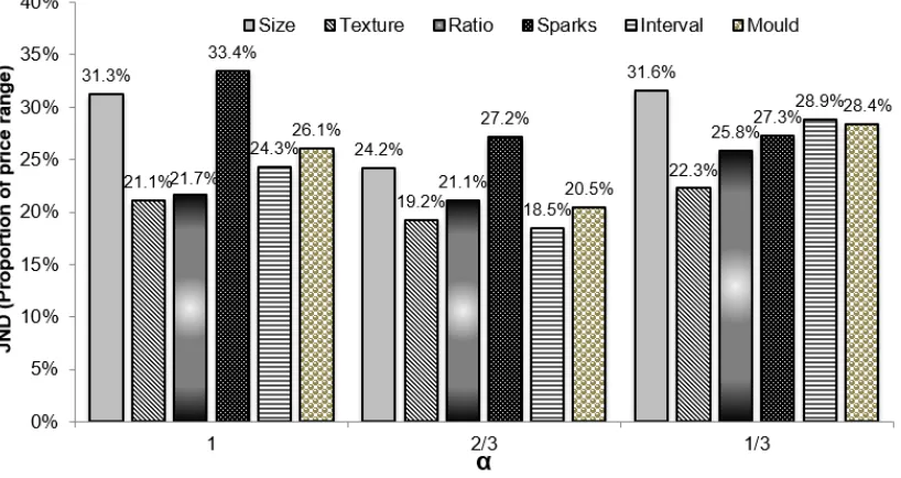
of a specific attribute and a specific α. Figure 4 presents estimated JNDs by attribute, j and

condition,c.

Figure 4: Average JNDs and acrossα condition and attributes.

Note: JNDs estimated from MEL model with dummies for each attribute and level ofα, plus interactions between the two.

Three findings are of note. The first is the level of absolute performance. Even with a single,

easily perceptible attribute related monotonically to price, surplus identification was imprecise. To

identify a surplus reliably, participants required it to exceed 18% of the price range, with a mean

discrimination (c.f., Figure 3), suggesting that imprecision did not result from perceptual noise.

Third, the non-linearity in the attribute-price relationship had little impact. In fact, there was a

slight advantage for the moderate diminishing returns case,α= 2₃.

Relative to imprecision, observed biases were small, The PSE was always in the region of 0-5

percentage points, albeit with a slight overall negative bias. On average, participants judged that

the surplus was zero when the product was, in fact, worth 1.5 percentage points less than the

displayed price.

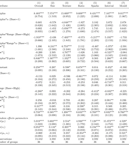
Table 1 provides a more detailed picture. Column (1) presents an overall model, aggregated

across attributes. The coefficient on the surplus is of course highly significant. The remainder

of the top half of the table presents interactions that test the impact of conditions on precision.

There was no overall effect of either non-linearity. The low attribute range had a modest negative

effect on the precision of surplus identification, although less so in the case of moderate diminishing

returns (α= 2₃). Precision was also influenced by location in the price range. The variable ‘Z-price’

corresponds to the display price expressed in standard deviations. The positive coefficient implies

that participants were somewhat more precise in the upper part of the price range.

The constant and its interaction terms indicate how the bias varied across conditions. The

positive coefficient confirms the slight general tendency to overestimate surplus. However, the

much larger effect was how the extent of bias varied across the price range. The positive coefficient

on Z-price shows that participants underestimated surpluses at the bottom of the price range and

overestimated them at the top.

Columns (2)-(7) estimate the model separately for each attribute.11 Variability in precision by

non-linearity and range was unrelated to perceptual discrimination, but followed a more complex

pattern. The advantage of moderate diminishing returns when the attribute range was low was

driven by two attributes only: the size and texture of the Golden Egg. Improved precision at higher

prices occurred for four of the six attributes. These inconsistencies may partly reflect idiosyncratic

aspects of the price ranges chosen for the three hyperproducts, such as the locations of salient round

prices, or may indicate non-linearities inherent in the perceptual coding of attribute magnitudes.

Nevertheless, four results were consistent across attributes: (1) surplus identification was imprecise;

(2) there was no advantage for linear over non-linear mappings of attributes to prices; (3) surpluses

11

Table 1: Mixed Effects Logit: Baseline models by attribute

(1) (2) (3) (4) (5) (6) (7)

Attribute Overall Size Texture Ratio Sparks Interval Mould Surplus 8.483*** 7.574*** 15.669*** 9.609*** 8.431*** 7.167*** 9.017***

(0.754) (1.519) (0.952) (1.225) (2.099) (1.991) (1.067) Surplus*α(Base=1)

2

3 0.685 -0.578 -4.048*** -1.827 3.182 3.872 2.878

(0.620) (1.642) (1.426) (2.005) (2.305) (2.692) (1.924)

1

3 0.002 -1.452 -5.056*** -0.273 1.745 3.142 0.643

(0.935) (1.667) (1.278) (1.680) (2.474) (3.557) (1.623) Surplus*Range (Base=High)

Low -1.919*** -2.438 -7.403*** -0.573 -5.217** 5.192** -1.733 (0.666) (2.105) (1.845) (1.781) (2.203) (2.153) (1.934) Surplus*Range*α(Base=1)

Low*2₃ 1.390 6.241** 6.753*** 2.112 -0.467 -5.375* -2.591 (1.001) (2.580) (2.248) (2.740) (2.752) (2.962) (2.689) Low*1

3 -0.200 2.505 4.767** -1.626 1.163 -8.525** -2.084

(1.073) (2.532) (2.139) (2.349) (3.066) (4.345) (2.643) Surplus*Z-price 0.846*** 1.567*** 1.332** 1.312* 0.383 1.266** -0.109 (0.209) (0.362) (0.605) (0.722) (0.584) (0.623) (0.667) Constant 0.258*** 0.267 0.598* 0.678*** 0.014 0.452* -0.160 (0.095) (0.188) (0.306) (0.161) (0.180) (0.252) (0.265)

α(Base=1)

2

3 -0.153 0.029 -0.596 -0.861*** 0.072 -0.114 0.280

(0.104) (0.272) (0.458) (0.180) (0.259) (0.337) (0.345)

1

3 -0.072 0.211 -0.253 -0.253 0.046 -0.718** 0.311

(0.108) (0.345) (0.513) (0.186) (0.405) (0.301) (0.318) Range (Base=High)

Low -0.280* 0.093 -0.202 -0.264 -0.412* -0.832** -0.225 (0.145) (0.222) (0.344) (0.203) (0.224) (0.387) (0.389) Range*α(Base=1)

Low*2

3 0.256 -0.016 0.793 -0.261 0.287 0.981** 0.236

(0.194) (0.387) (0.572) (0.262) (0.448) (0.444) (0.460) Low*1

3 0.317** 0.085 0.316 0.590* 0.315 0.569 0.205

(0.145) (0.344) (0.506) (0.348) (0.391) (0.486) (0.475) Z-price 0.733*** 0.565*** 1.208*** 0.632*** 0.769*** 0.832*** 0.760***

(0.064) (0.098) (0.104) (0.106) (0.101) (0.125) (0.109)

Random effects parameters

Var(µi) 5.019*** 5.602*** 2.554* 4.930*** 7.128*** 15.372*** 4.529*

(1.023) (2.088) (1.385) (1.770) (2.342) (4.753) (2.439) Var(υi) 0.052*** 0.116* 0.305** 0.060 0.194*** 0.183** 0.189***

(0.016) (0.064) (0.140) (0.059) (0.071) (0.072) (0.053) Cov(µi, υi) -0.069 -0.101 0.357 -0.354** -0.204 -0.175 0.521*

(0.095) (0.218) (0.222) (0.144) (0.263) (0.386) (0.317) Observations 15,552 2,592 2,592 2,592 2,592 2,592 2,592

Number of groups 36 36 36 36 36 36 36

were underestimated for low-value products and overestimated for high-value ones; (4) there was

heterogeneity across individuals, with the standard deviation across consumers equivalent to a

difference in JND of approximately 6 percentage points of the price range.12

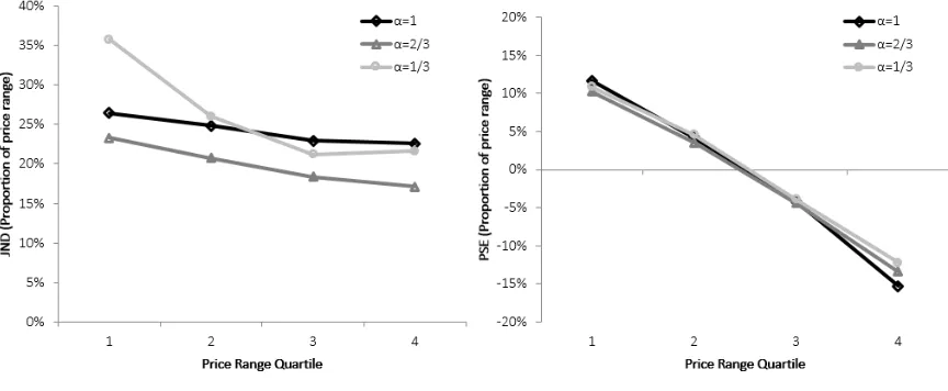
Figure 5 provides more intuition by presenting the estimated JND and PSE across price

quar-tiles, split by α condition. This confirms the modest improvement in precision at higher prices.

The JND for the first price quartile with severe diminishing returns (α= 1₃) stands out, suggesting

that when small changes in attribute magnitude translated into large changes in price,

percep-tual constraints evenpercep-tually reduced precision. However, changes in precision across the price range

were small compared to changes in bias, which were approximately linear and consistent across

conditions.

Figure 5: JND and PSE by α across price range

Note: The above estimates of the PSEs and JNDs are based on an estimated MEL that allows for all possible two-and three- way interactions between the price range quartiles,αconditions and the size of the surplus.

4.3.1 Learning

Trial number within each experimental run and its squared term were added to the baseline

spec-ification. Perhaps surprisingly, neither had a statistically significant impact on precision or bias

(p>0.25), indicating a lack of learning despite multiple exposures with feedback. To examine this

12

This is captured by the random effects parameter var(µi). While there was also variation in bias across individuals,

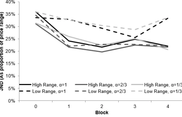
Figure 6: Average JND over time per experimental run.

Note: Each PSE is computed based on the parameter estimates from an MEL with non-linearity, range and block dummies specified, as well as their interactions. Block 0 refers to the initial 8 practice trials participants completed.

further, dummies separating each experimental run into four blocks of 18 trials were added to the

specification, which was also expanded to include a fifth block for the initial (non-incentivised)

practice trials (block 0). There was a statistically significant improvement in precision between the

practice and first block of test trials (p<0.001), but not thereafter. Although this difference may

reflect factors other than learning, such as participants experimenting with different strategies, the

implication remains that any learning was rapid. Figure 6 shows how JNDs evolved across

experi-mental runs for each α and range condition. For four of the six conditions, peak performance was

achieved after the practice trials, while for the other two learning was not robust.

A small learning effect did emerge over the whole experimental session (p<0.1), equivalent to

a decrease in JND of approximately three percentage points after 300 trials. This effect size is

small and its positive direction suggests that fatigue was not a factor. There was no equivalent

improvement in bias.

4.4 Discussion

The S-ID task produces quantitative measures of precision and bias in surplus identification. Facing

and systematically biased over the price range. Performance is clearly constrained by some form

of cognitive limitation.

The simplicity of the economic decision in Experiment 1 is important. Several recent models

that impose cognitive constraints on consumer choice hinge on how agents allocate limited attention

(Lipman, 1995; Sims, 2003), focus on a subset of relevant information (Bordalo et al., 2013; K˝oszegi

and Szeidl, 2013) or how they account for inevitable perceptual error (Woodford, 2012; Caplin and

Martin, 2015). Participants in Experiment 1 devoted their full attention to one salient attribute,

so allocation of attention across attributes was not involved. Similarly, attributes were designed

to minimise perceptual error. Indeed, the pilot study showed that relative magnitudes could be

perceived with high but variable precision across attributes. Contrastingly, surplus identification

was consistently imprecise. The limiting factor was, plainly, not perceptual in the sense of

dis-criminating relative magnitudes. Nor was performance affected by non-linear returns to attributes,

despite previous evidence that in some contexts consumers fail to account for non-linearities (see

Section 2).

Instead, the imprecision of surplus identification in Experiment 1 implies a more fundamental

limitation, the locus of which is neither perceptual, nor attentional, nor related to the shape of

returns. Rather, the ability to identify surpluses is limited by the need to compare relative location

on two otherwise incommensurate internal scales, one for monetary amounts, the other for attribute

magnitudes. The results suggest that internal representations of attributes can vary in granularity

(i.e., perceptual error) and linearity with only minimal impact on performance. Precision of surplus

identification is instead dominated by the mapping of one internal scale on to another, with limited

scope for learning once an initial mapping has been established. Such a constraint would explain the

consistent absolute level of performance, whereby the average observer requires a surplus equivalent

to one fifth of the price (or, equivalently, attribute) range for detection to be reliable.

An advantage of the S-ID task is that it generates separate measures of precision and bias. While

constraints in the mapping of incommensurate internal scales might explain uniform imprecision

across attributes, the consistent bias across the price range also requires explanation. Another

way to describe this bias is that, over trials, participants responded more to variation in attribute

magnitudes than to variation in prices. However, since this effect was independent of attribute,

might reflect a tendency for variation on a perceptual scale to be overestimated in comparison with

variation on a numeric one. This could happen if, for instance, the perceptual scale were subject to

visual contrast effects, leading differences in attribute magnitudes between successive presentations

to be exaggerated.

5

Experiment 2

The negligible impact of non-linear returns on surplus identification in Experiment 1 invites further

increases in the complexity of returns to attributes. The attribute-price relationships of everyday

products are frequently more elaborate than simple monotonic functions. What forms of complexity

might disrupt the uniformity of precision?

Experiment 2 increased the complexity, first, by incorporating a second attribute and, second,

by defining the attribute-price relationship via a range of more complex and economically interesting

functional forms, including some standard preference functions. (Hereafter we refer to the function

defining the attribute-price relationship as the “value function”.) These included functions with

increasing returns as well as non-monotonic and cyclical relationships.

The multi-dimensional attribute space also allowed us to test additional hypotheses arising

from Experiment 1. First, we reasoned that if biases when mapping attributes to prices result from

differences between the internal representations of visual and numeric quantities, a numeric product

feature would alter the bias. In half of the experimental runs, therefore, the magnitude of one of the

two attributes was presented numerically. Second, the use of numeric attribute magnitudes would

eliminate any error due to visual perception. Third, since adding a second attribute introduces

a new source of complexity in the form of the relative attribute weighting, we tested whether

performance was affected by relative weight. Lastly, and most straightforwardly, we hypothesised

that learning would be slower with more complex two-attribute products.

5.1 Method

Consumers from the Dublin area (N=24) were recruited through a market research company, with

approximate balance by gender (14 female), age (M=34.7, SD=13.0), and occupational status (54%

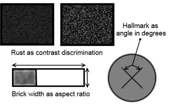
First, six additional attributes were employed.13 Three, one for each hyperproduct, were visual

(see Figure 7). On the Golden Egg, we varied a quality hallmark, the magnitude of which was

defined as the angle subtended by two intersecting lines. On the Victorian Lantern, we varied the

“rustiness” of the metal, defined as the contrast of an orange-brown versus black coloured texture.

On the Mayan Pyramid, we varied the flatness of the bricks, defined as the rectangular aspect ratio.

These visual stimuli were selected on the basis of the human ability to discriminate angle, contrast

and shape with relatively high precision.

Figure 7: Additional continuous attributes in Experiment 2

The other three attributes, again one for each hyperproduct, were numeric and appeared on

a label next to each hyperproduct (see figure 8). For the Golden Egg, we displayed the purity in

carats on a plinth; for the Victorian Lantern, fuel efficiency on a 25-point gradient scale; for the

Mayan Pyramid, age in years on a scroll.

Extending equation (2) to the two-attribute case,

Phtv =βh0+βh1fv(x1t, α1, x2t, α2) fv(·)∈[0,1] α1+α2= 1 (6)

wherevdenotes one of six value functions and theβs map the overall product magnitude,fv(·),

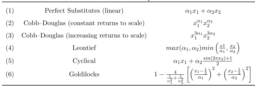
onto the price range for a given hyperproduct, h. Table 2 shows the six functional forms of fv(·),

which were designed to increase the complexity of the attribute-price relationship. Function (1) was

linear, with perfectly separable attributes. Function (2) had constant returns to scale overall, but

Figure 8: Numeric attributes in Experiment 2

diminishing returns (DRS) per attribute. Hence, these two value functions were equivalent to those

in Experiment 1, although with two-dimensions they differed with regard to separability. Function

(3) exhibited increasing returns (IRS) overall and for at least one attribute. Function (4) consisted

of a standard preference function in which attributes were perfect complements: the product was

as good as its weakest attribute (Leontief preferences). This specific form of complexity required

participants, first, to make a relative comparison of the attribute magnitudes and, then, to compare

the weakest against the displayed price. Function (5) combined one attribute with linear returns

with a more complex non-linear periodic attribute. We hypothesised that a cyclical attribute, with

more complex non-linear returns, would reduce precision and slow learning. Finally, function (6)

applied a non-monotonic non-linearity to both attributes, such that the centre of the attribute

space defined a perfect product. We called this the“goldilocks” value function, because the product

price corresponded to the distance in attribute space from the “just right” attribute levels.

Participants completed one run per value function. Each began with a learning phase in which

systematic examples of hyperproducts and prices were shown. In Figure 9, the order and locations

of the examples in attribute space are shown, together with indifference curves assuming balanced

attribute weights. Participants then undertook eight practice trials and 56 test trials (t). After

the product price,Phtz, was drawn (identically to Experiment 1), one combination of x1t and x2t

Table 2: Value function specifications

(1) Perfect Substitutes (linear) α1x1+α2x2

(2) Cobb–Douglas (constant returns to scale) xα1₁ xα2₂

(3) Cobb–Douglas (increasing returns to scale) x3₁α1x3₂α2

(4) Leontief max(α1, α2)min

x1 α1, x2 α2

(5) Cyclical α1x1+α2sin(2πx2₂ )+1

(6) Goldilocks 1− 4

1 α2₁+

1 α2₂

_x1−1

2 α1

2

+x2− 1 2 α2

2

(i.e., equally weighted, 1₂,1₂; b = 1) for half the runs and unbalanced (2₃,1₃ or 1₃,2₃; b = 2) for the

other half. Value functions, products, combinations of attribute pairs, and attribute balance were

all pseudo-randomised across participants and runs.

5.2 Results

MEL models were estimated following the specification in equation 1, with only the exogenous

variables zhtvb augmented. The baseline model included dummy variables for value function, v,

whether attributes were balanced, b, and interactions between the two.14 The results (Table 2,

column (1) and Figure 10) reveal that increasing the complexity of the value function disrupted

surplus identification.

Before examining this variation more closely, the absolute level of performance invites comment.

In Experiment 1, a single attribute range matched the full price range. In Experiment 2, on average,

the range of each attribute mapped on to only half the price range. The JNDs in Figure 10 are

measured, therefore, as a proportion of an attribute range, such that precision when an attribute

was mapped to price on its own can be compared directly to precision when a second attribute was

simultaneously taken into account. In Experiment 2, reliable surplus identification with the easiest

value functions required a surplus equivalent to one third to one half of an attribute range, compared

to one fifth to one quarter in Experiment 1 (Figure 4). The higher JNDs indicate substantial loss

of precision when the second attribute had to be considered simultaneously.

While overall precision was reduced, Figure 10 again reveals little difference between monotonic

14

Figure 9: Learning phases by price function

linear and non-linear value functions. The Leontief value function with balanced attributes was

the only condition to produce JNDs as low as Experiment 1. The more complex periodic and

goldilocks value functions resulted in substantially greater imprecision. Table 2, column (1) provides

significance tests. The slight deterioration in precision with increasing returns was marginally

outside conventional levels of statistical significance, while the improvement in the Leontief case

was significant only when attributes were balanced. However, the deterioration with non-monotonic

value functions was highly statistically significant.

Although the complexity of the value function had a strong impact, variation in the relative

weights of the attributes did not. Unbalanced attributes significantly disrupted the Leontief value

function only. The additional complexity introduced by this value function primarily surrounded

the need for participants to make two sequential judgements, first assessing relative attribute

mag-nitudes, then the relationship of the weakest attribute to price. It is likely that the first stage was

disrupted by unbalancing the attributes.

Table 3: Mixed Effects Logits: Testing for variable in ability across value function

(1) (2) (3) (4)

Surplus 4.668*** 4.277*** 4.796*** 4.361*** (0.437) (0.501) (0.466) (0.525) Surplus*Value Function (Base=Linear)

Constant Returns to Scale 0.171 0.413 0.218 0.499 (0.535) (0.574) (0.538) (0.563) Increasing Returns to scale -0.756* -0.643* -0.787* -0.651* (0.434) (0.380) (0.447) (0.381) Leontief 3.000*** 3.153*** 3.393*** 3.567***

(0.502) (0.428) (0.560) (0.476) Cyclical -1.862*** -1.820*** -1.876*** -1.828***

(0.436) (0.430) (0.448) (0.446) Goldilocks -2.577*** -2.440*** -2.671*** -2.517***

(0.380) (0.398) (0.355) (0.380) Surplus*Unbalanced Attributes -0.171 -0.003 -0.225 -0.021

(0.451) (0.418) (0.473) (0.427) Surplus*Unbalanced Attributes*Value Function (Base=Linear)

Lenotief -2.584*** -2.867*** -2.955*** -3.272*** (0.818) (0.787) (0.883) (0.839) Surplus*Numeric attribute 0.583*** 0.647***

(0.224) (0.237)

Surplus*Z-price 0.084 0.183

(0.145) (0.198) Surplus*Numeric attribute*Z-price -0.208

(0.252)

Constant 0.311 0.267 0.298 0.242

(0.217) (0.222) (0.223) (0.225) Value Function (Base=Linear)

Constant Returns to Scale -0.634** -0.613** -0.624** -0.598** (0.263) (0.258) (0.273) (0.266) Increasing Returns to scale -0.197 -0.186 -0.169 -0.154

(0.396) (0.388) (0.413) (0.404) Leontief -0.279 -0.269 -0.289 -0.274

(0.307) (0.303) (0.323) (0.317) Cyclical -0.407* -0.405* -0.387 -0.380

(0.233) (0.231) (0.244) (0.246) Goldilocks -0.670*** -0.663*** -0.695*** -0.684***

(0.255) (0.253) (0.262) (0.260) Unbalanced Attributes -0.407 -0.396 -0.408 -0.390

(0.266) (0.261) (0.279) (0.272)

Numeric attribute 0.072 0.091

(0.103) (0.106)

Z-price 0.490*** 0.443***

(0.053) (0.062)

Numeric attribute*Z-price 0.098

(0.091)

Random effects parameters

Var(µi) 1.670*** 1.694*** 1.834*** 1.865***

(0.419) (0.425) (0.451) (0.456) Var(υi) 0.011* 0.011* 0.016* 0.016*

(0.006) (0.006) (0.009) (0.009) Cov(µi,υi) -0.011 -0.010 -0.032 -0.029

(0.051) (0.052) (0.060) (0.060) Observations 8,064 8,064 8,064 8,064

Number of groups 24 24 24 24

Figure 10: JNDs across value function and attribute balance conditions

Note: Each JND was computed based on a MEL that included the magnitude of the surplus, value function dummies, and an unbalanced weight dummy, as well as all two-way and three-way interaction terms.

overvalued. The consistency of this effect across value functions is evident from Figure 11 and

its statistical significance from Columns (2)-(4) of Table 2. Contrary to our hypothesis that this

bias might be caused by visual contrast effects, the bias was somewhat larger in the presence of

a numeric attribute, as indicated by the positive interaction between numeric attributes and the

normalised display price (Z-price). The numeric attribute did generate a slight but significant

improvement in precision. Translating the coefficients from Table 2, when the visual attribute was

replaced by a numeric one, for a monotonic value function, the JND fell from approximately 42%

to 37% of the attribute range.

5.2.1 Learning

It is important to investigate whether deterioration in the precision of surplus identification reflected

cognitive limitations or slower learning. As in Experiment 1, adding the trial number and its squared

term to the baseline model yielded no effect. Including the practice trials in the estimation produced

Figure 11: Variation in the PSE across the price range.

Note: Each PSE has been computed based on the parameter estimates from an MEL with all value function dummies, price quartile dummies, and their interactions included.

(p<0.05) on its square, in keeping with a rapid asymptotic learning curve. This pattern was not

consistent across value functions, however. Performance actually deteriorated for the goldilocks

value function relative to the practice trials (p<0.05). Indeed, this effect was large: average JND

was 32.2% percentage points higher than during the practice trials. The need to make judgements

relative to an absolute benchmark, a “just right” point retained in memory, appears to have greatly

increased imprecision despite repetition and feedback.

As in Experiment 1, the bias across the price range did not diminish; in fact it strengthened

marginally over the session. In contrast to Experiment 1, there was no overall improvement across

the experimental session.

5.3 Discussion

Experiment 2 confirms and extends the findings of Experiment 1. In this simplified and

experimen-tally controlled environment, with training and feedback over many trials, surplus identification is

imprecise, biased and subject to only modest learning. The absence of an advantage for linear over

non-linearity is increased to include turning points, however, performance declines substantially.

Attributes that can be both too large and too small are common. Examples include portion sizes

for food and drink, terms of loans, engine sizes; consumers often seek a “happy medium”.

The systematic bias across the price range is unaffected by the use of a numeric attribute, which

suggests it does not result from contrast effects associated with visual attributes. We return to

alternative possible causes in the General Discussion. Numeric attributes can, it seems, make a

marginal improvement to the precision of surplus identification, suggesting perhaps a small role

for perceptual error, but with the dominant capacity constraint in surplus identification being the

need to map one internal scale on to another.

6

Additional Tests and Analyses

This section details additional tests and analyses designed to address two issues regarding the

gen-eralisability of our results. First, surplus identification may require learning over days rather than

an hour, especially for complex non-linear value functions, where lack of learning could reflect poor

understanding rather than limited information integration. To explore this possibility, we recruited

some highly numerate economics students to compete in a surplus identification tournament

span-ning more than a week. Second, one could of course question whether our results generalise to

subjective choices among more familiar products. The S-ID task imposes preferences upon

partici-pants via incentives to match a predetermined function. It is not certain that this process engages

the same evaluation mechanisms as the identification of purely subjective surpluses. However, the

richness of the S-ID task data allow some instructive additional tests. Specifically, we test whether

several biases repeatedly documented in subjective consumer choice tasks also appear in our data.

In addition, we test specific predictions of Woodford’s (2014) Optimal Sensor Model, which have

been confirmed in subjective choice data. Positive results, in these tests strengthen the case that

common psychological mechanisms underpin responses in the S-ID task and subjective consumer

choices.

6.1 Additional test: send in the experts

Employing the experimental design of Experiment 2, a small group of economics undergraduates

were highly numerate and understood iso-value curves. Prior to each run, they were shown the

exact functional form offv(.), including graphical examples. Thus, any risk of misundersting was

eliminated. To increase opportunities for learning, value functions, attributes and weightings for

each participant remained the same across sessions; only presentation order varied. The experiment

was a tournament: the best performer won e50. Furthermore, participants were told before the third session that they would win e5 if performance in their third or fourth session improved on their first or second session respectively.

Figure 12 presents mean JNDs by value function across sessions. Surplus identification remained

imprecise, but JNDs were lower than for the sample of Dublin consumers, confirming this cohort’s

“expert” status.15 _{Reliable identification in the goldilocks case still required a surplus equivalent}

to half an entire attribute range, but precision for the periodic function approached that for the

monotonic functions. The main purpose of this additional test was to provide greater

opportuni-ties for learning, yet it remained modest. Over four sessions totalling 1,536 trials with feedback,

competing for meaningful rewards, there was a slight improvement in precision for the monotonic

value functions (p<0.05), but the effect was very small. Meanwhile, the large and systematic bias

across the price range was replicated (p<0.001) and immune to learning. Thus, while young, highly

numerate students can outperform a representative sample of consumers, imprecision and bias are

not easily overcome. The only outstanding query from this exercise is the better relative precision

with the periodic value function. While we cannot be sure, participants seemed to find the

graphi-cal presentation particularly helpful, perhaps allowing them to match turning points to prices more

easily.

6.2 Tests for biases in common with subjective choice tasks

The S-ID task mimics the situation where a consumer encounters a new product and begins to learn

its worth. Yet the cost of gaining complete scientific control over attributes, prices and surpluses is

the need to impose preferences. If the S-ID task data were to contain similar patterns to those seen

in subjective consumer choice experiments, however, this would support the contention of common

psychological mechanisms. We therefore tested our data for some specific biases previously observed

in choice experiments.

15

Figure 12: JNDs across sessions for our expert sample

Note: Each JND has been computed based on the parameter estimates from an MEL with all value function dummies, session number dummies, and their interactions included.

6.2.1 Dilution and familiarity effects

Consumers often struggle to ignore irrelevant attributes. Meyvis and Janiszewski (2002) call this

the “dilution” effect and demonstrate across ten studies that irrelevant information alters consumer

product appraisals. The data from Experiment 1 are ideal for testing for dilution, because

partici-pants focused on one attribute while an irrelevant one varied randomly. Half the time, the attribute

to be ignored had been relevant on a previous run. We therefore added to the baseline MEL model

(Table 1, column 1) variables for the price signalled by the irrelevant attribute, for whether it had

been previously relevant and for the interaction between the two. Consistent with dilution, the

higher the value signalled by the irrelevant attribute, the greater the probability that the

partic-ipant perceived a surplus (p<0.01).16 Interestingly, the interaction term was non-significant; the

effect did not depend on whether the attribute had previously been relevant. This may reflect the

design of the hyperproducts, because attributes were selected to make intuitive sense, e.g., bigger

16_{It is important to note that because our method permits the separation of bias and precision in surplus}

eggs were more valuable, rusty lanterns less, etc.

6.2.2 The attraction effect

The “attraction effect” refers to the greater likelihood of choosing a product that dominates another

on all attributes (Huber et al., 1982) and has been demonstrated for both matching and choice tasks

(Tversky et al., 1988). Although in our experiments only one product was visible during any one

trial, trials were sequential and the relationship between the attribute magnitudes of successive

products was essentially random. Hence, in Experiment 2, for some trials the product was better

on both attributes than the previous one, thereby dominating it. Conversely, for some others it

was dominated. We tested whether participants were biased by domination relative to the previous

product, by adding two dummy variables to the baseline model. There was indeed an attraction

effect: domination of the previous product exaggerated perceived surplus (p<0.05), while being

dominated by it diminished perceived surplus (p<0.1).

6.2.3 Loss aversion

Loss aversion was first formalised and investigated empirically by Kahneman and Tversky (1979).

An extensive literature has explored asymmetries in how humans and animals weight losses and

gains in choices. While explanations for these empirical phenomena remain controversial, replicable

findings that imply loss aversion in economic choice are numerous (Rick, 2011; Ericson and Fuster,

2014).

Each successive presentation in the S-ID task entails an increase or decrease in attribute

mag-nitude relative to the previous product (and feedback price). To the extent that the most recently

perceived attribute provides a reference point, loss aversion implies a downward bias in perceived

surplus on trials when the attribute magnitude decreased, compared to those when it increased,

all else equal. Experiment 1 offers an ideal test, as successive presentations varied in a single

monotonic attribute. We added to the baseline model a variable for the standardised change in

attribute magnitude relative to the previous product, interacted with a dummy to indicate a

de-crease or an inde-crease. This revealed a highly significant contrast effect: the difference in successive

magnitudes was exaggerated (p<0.001). Furthermore, there was a significant interaction with the

the PSE is shown in Figure 13. The contrast effect for decreases in attribute magnitude was slightly

more than twice that associated with equivalent increases, as is typically observed in studies of loss

aversion in choice experiments.17

Figure 13: PSEs for changes in price relative to previous product.

Note: PSE was computed from parameter estimates from an MEL model including the standardised difference in attribute magnitude between the current and previous product, interacted with a dummy variable indicating whether the difference was positive (gain) or negative (loss). Interaction terms and standardised display price (Z-price) were included as controls.

6.3 Testing predictions of Woodford (2014)

Woodford (2014) demonstrates that his Optimal Information Constrained Model (OICM) of discrete

choice predicts patterns of response times when individuals choose between food items (Krajbich

et al., 2010). Although our experiments were not designed explicitly to test this model, there are

two reasons to check for consistency with the OICM. First, consistency would support a broader

application of the OICM model. Second, finding a similar pattern of response times in the S-ID task

would again suggest common mechanisms underpinning responses in the S-ID task and subjective

consumer choice.

17