Numerical solutions of diffusion-controlled moving
boundary problems which conserve solute
T.C. Illingworth, I.O. Golosnoy
*Department of Materials Science and Metallurgy, University of Cambridge, Pembroke Street, Cambridge CB2 3QZ, United Kingdom
Received 4 November 2004; received in revised form 2 February 2005; accepted 2 February 2005 Available online 23 May 2005
Abstract
Numerical methods of finding transient solutions to diffusion problems in two distinct phases that are separated by a moving boundary are reviewed and compared. A new scheme is developed, based on the Landau transformation. Finite difference equations are derived in such a way as to ensure that solute is conserved. It is applicable to binary alloys in planar, cylindrical, or spherical geometries.
The efficiency of algorithms which implement the scheme is considered. Computational experiments indicate that the algorithms presented here are of first order accuracy in both time and space.
Ó2005 Elsevier Inc. All rights reserved.
MSC:65P05; 65M06; 80A22
Keywords: Diffusion; Modelling; Conservation; Phase change; Moving boundary
1. Introduction
For physical systems of inhomogeneous composition, diffusion is often observed to cause a change of phase, even in material held at a constant temperature. Understanding these phase changes is important, since the microstructure of an alloy can have a profound effect on its properties. They are also central
to many engineering processes, including the homogenisation of layers of foils [1] or powder blends [2]
and the solidification ofÔtransientÕliquid phases[3,4]. Phase changes can equally be induced by the diffusion of solute from some external source. Although the conditions of these processes are rather different, they are equally industrially important, arising, for example, in problems of gas storage[5], and in the surface
0021-9991/$ - see front matter Ó2005 Elsevier Inc. All rights reserved. doi:10.1016/j.jcp.2005.02.031
*
Corresponding author. Tel.: +44 1223 334 341; fax: +44 1223 334 567. E-mail address:[email protected](I.O. Golosnoy).
modification of particular components (either deliberately, through processes such as aluminisation[6], or unintentionally, as during the decarburisation of steels[7]).
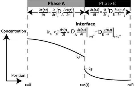
Diffusion-controlled phase changes can be described with reference to the situation drawn schematically in Fig. 1, where the concentration of solute (c) varies with position (r). Differences in chemical potential
Nomenclature
c=c(r,t) concentration
cA=c(s(t),t) equilibrium concentration of phase A in contact with B
cB=c(s(t)+,t) equilibrium concentration of phase B in contact with A
c1= c(1,0) far field concentration
DA=DA(c(r,t)) diffusion coefficient in phase A
DB=DB(c(r,t)) diffusion coefficient in phase B
k geometrical constant
M,N number of discretisation points
p=p(u,t) concentration (in phase A) q=q(v,t) concentration (in phase B)
r position
R position of far boundary
s=s(t) interface position
_
s¼s_ðtÞ ¼dsðtÞdt interface velocity
t time
u proportional position (in phase A)
v proportional position (in phase B)
dv spacestep (in phase B)
k constant related to geometry of system (1, 2 or 3 for planar, cylindrical or spherical,
respec-tively)
r constant between 0 and 1
j growth rate constant
[image:2.544.156.393.483.638.2]Subscripts are used to denote discretisations of space Superscripts are used to denote discretisations of time
energy are likely to be associated with such inhomogeneities, providing a driving force for the diffusion of matter. Composition profiles in each phase therefore also depend on time (t).
It is routine to use differential equations, commonly calledÔFickÕs lawsÕ, to model the way in which
com-position profiles evolve under the influence of diffusion[8]. Formulae of this type have been the subject of
much research and are well understood. However, in the present context, the analysis is complicated by the fact that diffusive processes occur simultaneously in two distinct phases.
The concentration of one phase in contact with the other is generally fixed by a thermodynamic con-straint. But the rate at which solute diffuses towards the interface through phase A and the rate at which it is removed into phase B are not necessarily equal. In order to conserve solute, therefore, the interface between the two phases must move. Writing the interface position ass=s(t), the following set of differential
equations can be used to model the complete system[9]:
rk1ocðr;tÞ
ot ¼ o or r
k1D
Aðcðr;tÞÞ ocðr;tÞ
or
; 06r6sðtÞ; ð1Þ
rk1ocðr;tÞ
ot ¼ o or r
k1D
Bðcðr;tÞÞ ocðr;tÞ
or
; sðtÞ6r6R; ð2Þ
DAðcðr;tÞÞ
ocðr;tÞ
or
r¼sðtÞ
DBðcðr;tÞÞ ocðr;tÞ
or
r¼sðtÞþ
¼ ½cBcA
dsðtÞ
dt ; r¼sðtÞ. ð3Þ
The first equation describes diffusion to the left of the interface, in phase A; the second equation refers to diffusion in phase B, to the right of the interface; the third describes the moving boundary condition at the interface, and is derived by requiring that solute be conserved there (subject to the assumption that it is at local equilibrium i.e. the concentrations are given by the equilibrium concentrationscAandcB). Together,
they form a coupled system of non-linear differential equations.
AlthoughFig. 1illustrates the planar case, these formulae can be applied to any geometry for which a
single parameter is sufficient to describe a location unambiguously. Eqs.(1)–(3) can therefore be used to
describe cylindrically or spherically symmetric systems, where radial distances define positions uniquely.
k= 1, 2 or 3 is a parameter which describes the geometry of the system (planar, cylindrical or spherical,
respectively).
Many of the situations in which diffusion-controlled phase changes are encountered typically involve isothermal conditions. In order to model these processes, it is therefore reasonable to assume that the
diffusion coefficients in Eqs.(1) and (2) are functions of composition only, and the equilibrium
concen-trations in Eq.(3) are constant. Evidently, it is possible to construct models that can describe the behav-iour of a system under non-isothermal conditions, or which incorporate the effects of heat flow. However, the scope of the present work is limited to the isothermal case. In addition, the Gibbs–Thompson effect will be neglected.
To complete the expression of the diffusion-controlled moving boundary problem, conditions at the fixed boundariesr= 0 andr=Ras well as initial conditions must be stated. For the modelling of processes such as homogenisation, zero-flux boundary conditions are most appropriate. A consequence of such conditions is that the solution must conserve solute. This is the case that will be considered in the present work. The most suitable initial conditions depend on the nature of the phase-change that is to be modelled. For the kind of homogenisation operations described above, the concentration at every point lies in a one-phase region of the phase diagram. But many metallurgical applications involve initial compositions that lie in the unstable two-phase region. In precipitation reactions, for example, a stable phase region grows from
a supersaturated matrix (whose concentration lies somewhere betweencAandcB).
Some closed form solutions to Eqs.(1)–(3)are known[10,11]. However, these formulae are only valid if
the diffusion coefficientsDAandDBare assumed to be independent of concentration. In addition, they are
solution can admittedly be extended to cover the case where neither of the phases is of zero initial size in planar geometries).
Such highly restrictive conditions mean that it is not possible to construct an analytical model of many situations that are of practical or industrial importance. In particular, the finite boundary conditions which are experienced by most real-life applications preclude any such attempt. Recourse must be made to
numer-ical methods of approximating the exact solution to Eqs.(1)–(3) instead.
2. Numerical solution techniques
Systems of differential equations with moving boundaries (also known as Stefan problems) arise in a variety of modelling situations across the sciences; many attempts have been made to solve them numeri-cally, as Crank has reported in great detail[12]. Furzeland, however, has noted that the most effective
ap-proach to solving a Stefan problem depends on the exact nature of the problem itself[13].
Many of the existing models developed specifically to describe diffusion-controlled phase changes have been limited to the planar geometry. This constitutes the simplest case, yet is sufficient to model certain
interesting applications, including transient liquid phase bonding[3]. The numerical techniques that have
previously been developed can be broadly distinguished by considering the way in which they discretise space.
The simplest methods[14,15]solve the diffusion equations(1) and (2)by discretising space with a fixed
mesh and imposing the requirement that the modelled position of the interface coincides with one of dis-cretisation points. This constrains the motion of the interface: it can only move in a step-wise manner, the nature of which is determined by the discretisation scheme. As well as being physically unrealistic, this approximation might additionally be expected to give rise to significant errors, since inaccuracies in esti-mated interface positions will directly affect the predicted behaviour of the system.
By including the interface position as a continuous variable in the model and solving a finite-difference form of Eq.(3)to predict its motion, it is possible to overcome this problem. Shinmura et al.[16]did this to investigate possible interlayer materials for bonding nickel. A similar model was developed by Zhou and North[17], who additionally introduced a quadratic expression for the concentration profile near the inter-face (in an attempt to better estimate the fluxes there and thus improve the accuracy of their method).
Extensions to include ternary systems have been implemented by Sinclair et al. [18], and the modelling
of moving boundaries in cylindrical and spherical geometries is possible using the commercially available
DICTRA code[19]. However, the precise mathematical details of this last algorithm remain rather unclear.
Difficulties in tracking the motion of the interface arise because of the discontinuity in the concentration profile there. Since the chemical activity of each species varies continuously across the sample, describing the way in which diffusion affects activity (rather than concentration) could potentially overcome these problems. Then, interface positions could be extracted from the predicted activity profiles, negating the need to describe the interface position explicitly (and therefore simplifying the analysis)[20]. Existing imple-mentations of schemes based on this concept have been found to agree very well with known analytical solutions[21,22].
the governing equations(1)–(3)in terms ofr(c,t) instead ofc(r,t). Unfortunately, in this new co-ordinate
system, the boundaries atr= 0 andr=Rare no longer fixed. This approach does not, therefore, simplify
the problem.
On the other hand, the transformations proposed by Landau[24]do introduce a co-ordinate system in
which all of the spatial boundaries are fixed. Numerical techniques based on this idea were first developed
by Murray and Landis in 1959 [25], although applications to the modelling of diffusion-controlled phase
changes came later, in the pioneering work of Tanzilli and Heckel[9]. Since then, the theory has been
ex-tended to include situations involving more than two species[26], more than one interphase boundary[27]
and concentration-dependent diffusion coefficients[28].
The Landau transformation involves two new positional variables (one for each phase). If phase A ex-tends fromr= 0 tor=s(t) (as shown inFig. 1),u¼ r
sðtÞfixes the extent of phase A to the domain 06u61. Writingp=p(u,t) to denote the concentration in terms of this new positional variable (which coincides with c(r,t) in phase A), the diffusion equation(1) can be written as[12]
½usk1 op
ots_ u s
op ou
¼ o
ou
½usk1DA
½s2
op ou
!
; 06u61; ð4Þ
where_s¼s_ðtÞ ¼dsðtÞ
dt.
For phase B, the domain r=s(t) to r=R can be described as 06v61 if v¼rsðtÞ
RsðtÞ. Writing q=q(v,t) =c(r,t) to denote the concentration in this new co-ordinate system, the diffusion equation (2)
can be written as
½vðRsÞ þsk1 oq
ots_
1v
Rs
oq ov
¼ o
ov
½vðRsÞ þsk1DB
½Rs2
oq ov
!
; 06v61. ð5Þ
The transformed version of the interface equation(3) is
DA
s op ou
u¼1
DB
Rs
oq ov
v¼0
¼ ½cBcA
ds
dt; u¼1; v¼0. ð6Þ
Although the new co-ordinate system has rendered the governing equations(4)–(6)into a form more
com-plex than(1)–(3), it has simplified the problem in that all of the boundaries are now fixed. Consequently,
any of the advanced numerical methods originally developed to solve systems of partial differential equa-tions with fixed boundaries can be applied to the problem. Since these methods are well understood, it might be anticipated that accurate solutions will be found more easily using the transformed co-ordinate system than would otherwise be the case.
A further advantage of using transformed space is that a constant (time-invariant) discretisation ofuand
vcorresponds to points whose position (in real space i.e. in therco-ordinate system) actually varies. In
other words, the mesh automatically adjusts itself to accommodate the motion of the interface, as shown inFig. 2.1It is therefore possible to introduce a non-uniform spatial discretisation that has a higher reso-lution in locations where large concentration gradients are expected (for example, near the interface). This can lead to improvements in the accuracy of an algorithm without compromising its efficiency.
The majority of the numerical models referred to above solve equations(1)–(3)(or, equivalently,(4)–(6)) with finite difference expressions that are explicit in nature. There are consequently limitations of the size of timestep which can be used to find a numerically stable solution. Accurate calculations therefore require a large computational effort.
1 Note that this is not anÔadaptive meshÕinasmuch as the location of the discretisation points corresponds to fixed values ofuandv;
In order to overcome this limitation, it is possible to construct implicit finite difference schemes that are stable for any timestep. However, this is not trivial, since the future interface position depends on future
composition profiles (and vice-versa). In other words, Eqs.(1)–(3)form a coupled set of equations. It
fol-lows that any implicit scheme must consider all three equations simultaneously. Since the interface equation
(3)is not linear, the entire problem involves solving a large system of non-linear equations at each timestep. This is potentially very demanding in terms of computing time. It follows that implicit schemes would not necessarily model moving boundary problems very much more efficiently than explicit methods.
A more fundamental problem with the existing algorithms is that none of them conserve solute.2It is
true that the way in which Eqs. (1)–(3) (or, equivalently, (4)–(6)) were derived means that it is possible
to ensure that solute is conserved (by imposing zero-flux conditions atr= 0 andr=R). However, the finite
difference schemes used to approximate the governing equations have, in all cases, resulted in numerical solutions which do not conserve solute. This problem has previously been identified by Crusius et al.
[image:6.544.170.381.93.393.2][29]and further investigated by Lee and Oh[30].
Fig. 2. The Landau transformation introduces new positional variables for which the interval [0,1] corresponds to the extent of one of the phases. A fixed discretisation of these variables therefore corresponds to points whose position in real space can be considered to be automatically adjusting to accommodate the motion of the interface.
2 This is not true of the enthalpy methods based on a description of the chemical activity gradients (rather than concentration); but
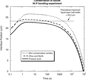
As an example of this effect, consider the predictions of Zhou and North [17], which are reproduced in Fig. 3. In order to model the bonding of nickel using Ni–P interlayers, they calculated how the half-thickness of a liquid layer varies whencA= 10.223 at.% and cB= 0.166 at.%. If the initial thickness and
concentration of phase A is 12.5lm and 19 at.%, respectively, and if phase B initially contains no solute,
it is possible to calculate aÔtheoreticalÕ maximum thickness for the liquid layer: approximately 23.2lm.
ThisÔmaximumÕ is exceeded by the numerical calculations, as can be ascertained fromFig. 3. The same is true of results generated from a model based on the Landau transformation and a standard discretisation of Eq.(6) [12], which was run using the same input parameters (DA= 500lm2s1, DB= 18lm2s1and
R= 3012.5lm) and a similar initial step size (1lm) and time step (0.01 s).
It is emphasised that non-conservation of solute is an inherent problem with existing numerical schemes, and is not simply a consequence of computational inaccuracies such as rounding errors. It arises because the numerical approximations used to calculate the fluxes near the interface when solving the interface
equation(3)are different to those used when approximating the diffusion equations(1) and (2). The extent
to which a numerical solution gains or loses solute depends on the precise nature of the finite difference forms used. In generally, it is non-negligible and is particularly large when large concentration gradients are present in the system[29,30]. Some authors have even used this value to estimate the accuracy of their calculations[28].
Non-conservation of solute is clearly a source of inaccuracy in any numerical model, since the exact
solutions to Eqs. (1)–(3) satisfy the physical requirement that matter must be conserved. Yet the
accu-racy of existing schemes is a question that has not been addressed in any great detail. Certainly, the
0 5 10 15 20 25 30
0.1 1 10 100 1000 104 105
Conservation of solute Ni-P bonding experiment
Zhou and North Non-conservative Landau
Present work
In
r
etf
e
c
ai
s
o
P i
tn
o(
µ
)
m
Time (s)
Theoretical maximum liquid layer half-width
[image:7.544.128.409.354.617.2]= 23.2µm
amount of solute lost or gained is related to the type of mesh that is used (as well as the details of the numerical scheme). If errors associated with non-conservation are to be limited, it is necessary to fix a maximum allowable timestep. Instead of identifying this maximum, previous workers have generally simply conducted calculations using rather fine discretisations of time. Restrictions of this type are re-quired both for implicit and explicit schemes, and will obviously affect the efficiency of any non-con-servative algorithm.
By using alternative finite difference approximations for Eqs.(1)–(3), it is possible to reduce the errors
associated with non-conservation for both fixed mesh[29]and moving mesh[30]methods. However, none
of the proposed improvements actually render the algorithms conservative of solute. The authors of the present work have previously shown that conservative schemes can be derived by adopting a different ap-proach to modelling the interfacial fluxes [31].
These improvements are limited to the planar geometry. Here, a conservative scheme which describes the behaviour of the diffusion-controlled moving boundary problem in cylindrical and spherical geometries is developed. The resulting fully implicit algorithm can calculate solutions to a known accuracy for any space-step or timespace-step.
3. A conservative scheme
3.1. Derivation
Existing methods of solving the two-phase diffusion problem use finite difference forms based on the
differential equations (3)or (6)to model the motion of the interface. But all such numerical schemes fail
to conserve solute. In order to derive conservative forms, instead of solving for the motion of the
inter-face directly, consider the total amount of solute present in the system. At any time t, this quantity is
given by Z sðtÞ
0
cðr;tÞkrk1drþ
Z R
sðtÞ
cðr;tÞkrk1dr¼ksðtÞ
Z 1
0
pðu;tÞ½usðtÞk1duþkðRsðtÞÞ
Z 1
0
qðv;tÞ½ðRsðtÞÞvþsðtÞk1dv;
wherekis a geometrical constant (k= 1 for the planar case, 2pfor the cylindrical and 4pfor the spherical). For the total amount of solute in the system to remain constant, this value must be time-invariant:
o ot sðtÞ
Z 1
0
pðu;tÞ½usðtÞk1duþ ðRsðtÞÞ
Z 1
0
qðv;tÞ½ðRsðtÞÞvþsðtÞk1dv
¼0. ð7Þ
In order to calculate a solution based on this expression, it is necessary to modify the diffusion equations too. To do so, note that the identities
oðps½usk1Þ
ot s½us
k1op
otþp½us
k1
_
sþpsðk1Þ½usk2us_ and
oðpu½usk1Þ
ou u½us
k1op
ouþp½us
k1
þpuðk1Þ½usk2s
can be used to express Eq.(4)as
o otðps½us
k1
Þ ¼ o
ou ½us
k1
_
spuþDA
s op ou
Similar identities can be used to cast Eq.(5)intoÔdivergentÕ form:
oðqðRsÞ½vðRsÞ þsk1Þ
ot ¼
o
ov ½vðRsÞ þs
k1
_
sqð1vÞ þ DB
Rs
oq ov
; 06v61. ð9Þ
In the same way that Eqs.(1)–(3)or(4)–(6)provide a complete mathematical description of the two-phase
diffusion-controlled moving boundary problem, the physical requirements of the system are fully expressed by Eqs.(7)–(9), though the interface equation is now expressed in an integral form (as opposed to a differ-ential form). The new formulation is more complicated than both those presented in the previous section, but it will be shown presently that they can be used to derive a finite difference scheme which conserves solute (and which might therefore be expected to be more accurate).
In order to derive a finite difference scheme, space is discretised atM+ 1 points. The firstN+ 1 points are given by a fixed discretisation ofu, which corresponds to the extent of phase A. Using a subscript nota-tion to denote discretisanota-tions of space, the points in phase A are written asu0= 0,u1,. . .,uN= 1, as indicated
in Fig. 2. The last MN+ 1 points are in phase B and are given by a fixed discretisation of v (at vN= 0,vN+ 1,. . .,vM= 1). Discretisations of time will be indicated using superscripts (e.g.tj).
Now integrate the divergent form of the diffusion equations(8) and (9)around each node over one
time-step. In phase A, Z uiþ1=2
ui1=2 Z tjþ1
tj o otðpsðsuÞ
k1
Þdtdu¼
Z tjþ1
tj
Z uiþ1=2
ui1=2
o ou ðsuÞ
k1
_
spuþDA
s op ou
dudt
can be re-written as Z uiþ1=2
ui1=2
fpjþ1sjþ1ðsjþ1uÞk1pjsjðsjuÞk1gdu¼
Z tjþ1
tj
ðsuiþ1=2Þ
k1
_
spiþ1=2uiþ1=2þ
ðDAÞiþ1=2 s op ou i
þ1=2
! (
ðsui1=2Þk 1
_
spi1=2ui1=2þ
ðDAÞi1=2 s op ou
i1=2
!) dt.
Taking a constant,pji, to approximate the variablepj=p(r,tj) over the intervalui1þui
2 ¼ui1=26u6uiþ1=2
¼uiþuiþ1
2 (and similarly forp
jþ1
i ), it is possible to simplify the integral on the left hand side of this equation:
Z uiþ1=2
ui1=2
fpjþ1sjþ1ðsjþ1uÞk1pjsjðsjuÞk1gdup
jþ1
i
k fðr
jþ1
iþ1=2Þ
k
ðrjiþ11=2Þkg p
j i
kfðr
j iþ1=2Þ
k
ðrji1=2Þkg;
where the notationrji1=2 is used forsjui± 1/2.
To discretise the right hand side of the equation, introduce a parameterr, such that 06r61. Then, tak-ing a constantpjiþr ¼rpijþ1þ ð1rÞpjito approximate the concentration arounduiover the interval between
tjandtj+ 1, the integral can be solved to give the following finite difference scheme for diffusion in phase A:
1
tjþ1tj
pjiþ1
k fðr
jþ1
iþ1=2Þ
k
ðrjiþ11=2Þkg p
j i
k fðr
j iþ1=2Þ
k
ðrji1=2Þkg
" #
¼ ðrjiþþ1r=2Þk1 s_jþrpjþr
iþ1=2uiþ1=2þ
ðDAÞ
jþr
iþ1=2
sjþr
op ou
jþr
iþ1=2
( )
ðrjiþ1r=2Þk1 s_jþrpjiþ1r=2ui1=2þ
ðDAÞjiþ1r=2
sjþr
op ou
jþr
i1=2
( )
i¼1;2;. . .;N1. ð10Þ
To find the numerical scheme for phase B, Eq.(9)is integrated over one spacestep and one timestep. The
1
tjþ1tj
qjiþ1
k fðr
jþ1
iþ1=2Þ
k
ðrjiþ11=2Þkg q
j i
kfðr
j iþ1=2Þ
k
ðrji1=2Þkg
" #
¼ ðrjiþþ1r=2Þk1 s_jþrqjiþþ1r=2ð1viþ1=2Þ þ
ðDBÞjþ
r
iþ1=2
Rsjþr
oq ov
jþr
iþ1=2
( )
ðrjiþ1r=2Þk1 s_jþrqjþr
i1=2ð1vi1=2Þ þ
ðDBÞ
jþr
i1=2
Rsjþr
oq ov
jþr
i1=2
( )
i¼Nþ1;Nþ2;. . .;M1; ð11Þ
where nowrji1=2 is used for (Rsj)vi± 1/2sj.
The left hand side of Eqs. (10) and (11)correspond to the change in the amount of solute in element
i over the interval between t=tj and t=tj+ 1. This must be balanced by the right hand side, which re-lates to the difference between the amount of solute diffusing into the element and the amount diffusing
out (the terms involving D), corrected for the changing size of the element (the advection-type terms
involving s_).
To generate a finite difference form of the conservation equation(7), it is necessary also to derive finite dif-ference approximations for the concentrations at the boundaries (i= 0,NandM), where Eqs.(10) and (11)do not apply. At the moving interface, local equilibrium implies thatpjN ¼pNjþ1¼cA andqjN ¼q
jþ1
N ¼cB. For the
fixed boundaries, on the other hand, zero flux requirements op
ou
u
¼0¼0 and
oq
ov
v
¼1¼0
are imposed.
Inte-grating(8)betweenu0andu1/2and(9)betweenvM1/2andvM, it is possible to derive the relationships
pj0þ1
k fðr
jþ1 1=2Þ
k
g p
j
0
kfðr
j
1=2Þ
k
g ¼ ðrj1þ=2rÞk1 s_jþrpj1þ=2ru1=2þ
ðDAÞ
jþr
1=2
sjþr
op ou
jþr
1=2
" #
( )
ðtjþ1tjÞ and
qjMþ1
k fðRÞ
k
ðrjMþ11=2Þkg q
j M
k fðRÞ
k
ðrjM1=2Þkg
¼ ðrjMþr1=2Þk1 s_jþrqjMþr1=2ð1vM1=2Þ þ
ðDBÞ
jþr
M1=2
Rsjþr
oq ov
jþr
M1=2
" #
( )
ðtjþ1tjÞ.
These equations have been written in such a way as to include the untransformed co-ordinaterji. That
notation, which corresponds to the physical position of each node at each timestep, is used as shorthand for the following relationships:
rji¼
uisj if i<N;
sj if i¼N;
ðRsjÞv
iþsj if i>N.
8 > < > :
To discretise the interface equation(7), the integrals are converted to finite sums. The difference between the amount of solute in each element at timetj+ 1and the amount at timetjis given by terms such as
pjiþ1fðrjiþþ11=2Þk ðrjiþ11=2Þkg pjifðrjiþ1=2Þk ðrji1=2Þkg and
qjiþ1fðrjiþþ11=2Þk ðrjiþ11=2Þkg qjifðrjiþ1=2Þk ðrji1=2Þkg;
kðtjþ1tjÞðrjþr
N1=2Þ
k1
_
sjþrpjNþr1=2uN1=2þ
ðDAÞjNþr1=2
sjþr
op ou
jþr
N1=2
( )
þcAððsjþ1Þ
k
ðsjÞk ðrjNþ11=2Þkþ ðrjN1=2ÞkÞ þcBððr
jþ1
Nþ1=2Þ
k
ðrjNþ1=2Þk ðsjþ1Þkþ ðsjÞkÞ
þkðtjþ1tjÞðrNjþþr1=2Þk1 _sjþrqjNþþr1=2ð1vNþ1=2Þ
ðDBÞjþ
r
Nþ1=2
Rsjþr
oq ov
jþr
Nþ1=2
( )
¼0. ð12Þ
Eqs.(10)–(12)form a complete discretisation of the problem described analytically in Eqs.(7)–(9), subject to zero-flux boundary conditions. The way in which they were derived has ensured that solutions calculated numerically using these expressions will conserve solute. In view of the paucity of data regarding the way in which diffusion coefficients depend on concentration for the majority of chemical systems, the remainder of this work makes the simplifying assumption that they are constant.
3.2. Implementation
In order to calculate a numerical solution using Eqs.(10)–(12), particular approximations for the terms that fall between discretisation points (i.e. at times j+r and positionsi± 1/2) must be chosen. It is also necessary to determine a method of solving the resulting set of simultaneous equations. Since these ques-tions relate directly to the overall accuracy and efficiency of the algorithm, it is worth considering them carefully.
It is well known that explicit schemes (r= 0) only produce numerically stable solutions to diffusion prob-lems when the timestep is smaller than some critical value, whereas any value of the timestep can be used with implicit schemes for whichrP1/2[32,33]. It is also known that any partially implicit scheme
(includ-ing the Crank–Nicolson scheme (r= 1/2)) can give unphysical oscillations in cases where large
concentra-tion gradients are present[32,34].
Large gradients are typical of diffusion-controlled phase changes. In order to generate realistic solutions, a maximal timestep must therefore be imposed for a given discretisation of space. When the spacestep is small, this auxiliary condition can be more restrictive than the stability requirement, rendering the methods very inefficient. Since fully implicit schemes (r= 1) are not subject to such restrictions, attention in the remainder of this work is limited to algorithms of this kind, though the velocity term will be taken to be
_
sjþr¼sjþ1sj
tjþ1tj.
Unphysical, oscillating solutions can also be generated if approximations for the terms at intermediate positions are not chosen carefully. For example, non-monotonic profiles can be predicted if the centred-difference approximation,pjiþ11=2¼pj
þ1
i1þp
jþ1
i
2 , is used[34,35]. On the other hand, the first order up/down-wind
approximations:
pjiþ11=2¼pjiþ1;pijþþ11=2¼pjiþþ11if the velocity is positive (sj+ 1>sj),
pijþ11=2¼pijþ11;pjiþþ11=2¼pijþ1if the velocity is negative (sj+ 1<sj),
do not, no matter what kind of discretisation scheme is used[34,35]. It follows that this type of approxi-mation is preferable to centred-difference formulae, even though it is only of first order accuracy.
When substituted into Eqs.(10)–(12), a set of simultaneous equations is generated. These involveM+ 3 unknowns: the future concentrationspj0þ1;p1jþ1;. . .;pjNþ1;qjNþ1;qNjþþ11;. . .;qjMþ1and the future interface position sj+ 1. Since all of the equations are coupled, if the implicit scheme is to conserve solute, the entire system must be solved simultaneously. But the fact that they form a non-linear system means that this is potentially very demanding in terms of computing time.
be written as a tri-diagonal matrix equation, a form for which cheap inversion algorithms are available
[36].) Conversely, if future concentrations were known, the future interface position could be calculated
from Eq.(12)relatively easily.
For the planar case, the authors have already shown that it is possible to implement an efficient
algo-rithm based on de-coupling the problem in this way [31]. The approach amounts toÔcoefficient freezingÕ:
firstly, future compositions are calculated using some fixed estimate ofsj+ 1; in turn, the concentration pro-file is frozen and a corrected estimate for the future interface position is calculated. In order to improve the accuracy of the estimates, the process is then repeated.
An iterative algorithm that considers Eqs. (10)–(12)sequentially therefore obviates the need to solve a
large system of non-linear equations simultaneously. Nevertheless, the non-linear equation(12)must still
be solved at each iteration. Although it only involves one unknown, finding an exact solution is not trivial. Furthermore, any estimate is likely to be refined by further iterations. Therefore, rather than finding an
ex-act solution to Eq.(12)for a particular frozen concentration profile, it may be adequate simply to find an
approximate solution. In the planar case, for example, a linearised version of Eq.(12)was found to provide
a sufficiently accurate solution without otherwise affecting the algorithm[31].
A linearisation for the spherical case is constructed using some estimated future interface position,sj+ 1, and future concentrations, pjiþ1and qjiþ1. An approximate root (which can then be used as an improved estimate of the interface position) is given bysjþ1
, where
ðsjþ1
s
jÞ 3ðrjþ1
N1=2Þ 2
pjNþ11=2uN1=23ðr
jþ1
Nþ1=2Þ 2
qjNþþ11=2ð1vNþ1=2Þ þcAfððsjþ1Þ
2
þsjþ1sjþ ðsjÞ2
Þ ððrjNþ11=2Þ2
h
þrjNþ11=2r
j
N1=2þ ðr
j N1=2Þ
2
ÞuN1=2g cBfððsjþ1Þ2þsjþ1sjþ ðsjÞ2Þ ððr
jþ1
Nþ1=2Þ 2
þrjNþþ11=2r
j Nþ1=2
þðrjNþ1=2Þ2Þð1vNþ1=2Þg
i
¼3ðtjþ1tjÞ ðrNjþþ11=2Þ2 DB
Rsjþ1
qjNþþ11cB
vNþ10
ðrjNþ11=2Þ2DA
sjþ1
cAp
jþ1
N1
1uN1
" #
.
ð13Þ
The basis of an efficient algorithm for solving Eqs. (10)–(12)is now clear – at each timestep:
(1) Takepji;qji andsjas initial estimates ofpijþ1;qjiþ1andsj+ 1. (2) Calculatesjþ1
using Eq.(13).
(3) Updatesj+ 1using this value.
(4) Calculatepjiþ1and qjiþ1using the tri-diagonal matrices which result from(10) and (11)(along with the boundary conditions).
(5) Updatepjiþ1 and qjiþ1 using these values.
Steps 2–5 are then repeated until successive estimates of the interface positionsj+ 1differ by less than some fixed tolerance. If the series of estimates does converge to some fixed value, it will correspond to a solution of the implicit set of discretised equations(10)–(12).
Computer code implementing this fully implicit and conservative algorithm has been prepared for the
planar and spherical geometries (k= 1 and 3). In the planar case, de-coupling and linearising the problem
4. Results and validation
Before addressing any other issue regarding output from the algorithm, it is confirmed that the numer-ical scheme conserves solute (to within rounding accuracy) in every calculation. Consider, for example,Fig. 3, where it is used to predict how the interface position varies as a function of time for one particular planar system. All of the calculations use the same input parameters and the time- and space-step in both of the models based on the Landau transformation are the same. The traces are all qualitatively similar, with one significant difference: the new scheme does not predict that the thickness of the liquid layer will exceed the theoretical maximum.
The question of whether the solution is accurate remains. For particular initial and boundary conditions, analytical solutions are available to describe the motion of an interface which is driven by diffusion[10]. These are all based on ZenerÕs expression for the concentration profile in an infinitely large matrix phase
surrounding a homogenous growing phase region that is infinitely small at timet= 0 [11]. For this case,
the concentration profile is given by
cðr;tÞ ¼c1þ
ðcBc1Þ
IkðjÞ
Ik
r
ffiffiffiffiffiffiffiffiffiffi 4DBt
p
; IkðuÞ ¼
Z 1
u
v1kev2dv; ð14Þ
wherejis a constant that depends on the geometry of the system (i.e.k), as well ascA,cBandc1(the initial concentration of the matrix):
2jkI
kðjÞej
2
¼cBc1
cBcA
.
A concentration profile of this nature implies that the position of the interface moves in a parabolic manner:
sðtÞ ¼j ffiffiffiffiffiffiffiffiffiffi4DBt
p
. ð15Þ
The availability of an exact solution affords an opportunity to asses the accuracy of the numerical scheme. However, the exact solution describes the situation where one phase (A) is initially infinitely small and where the other (B) is infinitely large, whereas the numerical solution has been developed to describe a system in which there are two phases, each of which is of a finite size. Despite this apparent difficulty, it is still possible to compare the two models.
Firstly, note that the finite extent of phase B does not affect the behaviour of the system so long as there is no diffusion taking place at the far end (r=R). It is therefore appropriate to compare numerical and ana-lytical predictions atÔshortÕtimes (when the effect of the far boundary is not significant). Secondly, the size of phase A is only zero fort= 0. Therefore, if the numerical calculations are initialised using the exact solu-tion at some finite time (when phase A is of finite extent and homogenous in composisolu-tion), the algorithm can be used to solve the early stages of the problem for which analytical formulae are available. It is then possible to compare numerical results with the exact solution.
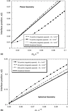
Numerical calculations have therefore been conducted for a system where atomic fractions of 0.4 and 0.2 are taken as values for the interfacial composition in phases A and B, respectively, and where the far-field value is 0.3. For a geometry whereR= 1 andDB= 1, the model was initialised using the exact profiles for a
time of 0.0001 (in the planar case) and 0.025 (in the spherical case) and run with a various meshes. Some of the associated results are presented inFig. 4.
According to Eq.(15), the interface position should vary with the square root of time. This behaviour is reflected in bothFigs. 4(a) and (b). However, there are some inaccuracies in the predictions. These arise due
to the finite difference approximations used for(4)–(6); naturally, the magnitudes of the errors depend on
In order to investigate the way in which particular choices for the timestep affect the accuracy of predic-tions, a very large number of nodes (10 000) was fixed, and calculations repeated for a various different timesteps. For each set of calculations, the difference between the numerical predictions and the exact solu-tion was calculated; associated data are presented inFig. 5. Further increases to the spatial resolution were
0 0.01 0.02 0.03 0.04 0.05 0.06 0.07 0.08
0.02 0.04 0.06 0.08 0.1
Planar Geometry
Analytical Solution
10 points (irregularly spaced) - t = 1x10⁻⁴ 10 points (regularly spaced) - t = 1x10⁻⁴ 100 points (regularly spaced) - t = 1x10⁻⁷
Interf
ace position, s(t)
Interf
ace position, s(t)
(a)
(b)
(DB t)1/2
0.1 0.15 0.2 0.25
0.05 0.06 0.07 0.08 0.09 0.1
Spherical Geometry
Analytical Solution
250 points (regularly spaced) -δt = 1x10⁻⁷ 25 points (irregularly spaced) -δt = 1x10⁻⁴ 25 points (regularly spaced) -δt = 1x10⁻⁴
[image:14.544.132.412.93.551.2](DB t)1/2
0 5 10-5 0.0001 0.00015 0.0002
0 0.002 0.004 0.006 0.008 0.01
Effect of timestep on accuracy of planar model
t = 4x10⁻⁵
t = 2x10⁻⁵
t = 1x10⁻⁵
)t
(
s
,r
or
r
E
u
nr
e
mi
c
a
l
)t
(
s
-
a
x
ec
t
D
(a)
(b)
Bt
0 0.0002 0.0004 0.0006 0.0008 0.001 0.0012 0.0014
0.003 0.004 0.005 0.006 0.007 0.008 0.009 0.01
Effect of timestep on accuracy of spherical model
δt = 4x10⁻⁵
δt = 2x10⁻⁵
δt = 1x10⁻⁵
)t
(
s
,r
or
r
E
u
ne
mr
i
a
cl
)t
(
s
-
a
x
ec
t
[image:15.544.124.412.90.622.2]DBt
0 0.0002 0.0004 0.0006 0.0008 0.001
0 0.002 0.004 0.006 0.008 0.01
Effect of spacestep on accuracy of planar model
400 points 200 points 100 points
)t
(
s
,r
or
r
E
u
ne
m
a
cir
l
)t
(
s
-
x
e
a
ct
D
(a)
(b)
Bt
0 0.0005 0.001 0.0015 0.002
0.003 0.004 0.005 0.006 0.007 0.008 0.009 0.01
Effect of spacestep on accuracy of spherical model
500 points 250 points 1000 points
)t
(
s
,r
or
r
E
u
nm
e
ri
c
a
l
)t
(
s
-
a
x
ec
t
[image:16.544.129.417.100.622.2]DBt
found to have no discernable effect on the accuracy of the algorithm, indicating that the errors shown in
Fig. 5are dominated by the coarse discretisation of time.
For both geometries, decreasing the timestep improves the accuracy of the model: halving the timestep decreases the error by a factor of approximately two. This demonstrates that the algorithm is first order accurate in time. In fact, the planar model performs rather better than that, as halving the timestep reduces the error by a factor slightly greater than two.
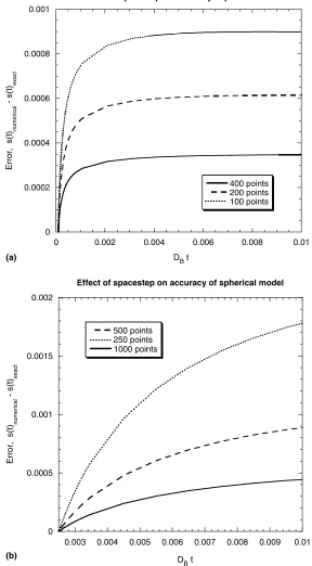
In Fig. 6, the error in the solution calculated by the numerical algorithm is shown for various
dif-ferent spacesteps. Because it uses a transformed co-ordinate system, the spatial variables u and v are
discretised rather than real space. Since the analytical solution with which the numerical model is being
compared is only valid when phase A is uniformly at its equilibrium concentration, cA, the behaviour
of the numerical system is determined purely by the spacing between nodes in phase B, dv. The results
clearly indicate that increasing the number of points in phase B (i.e. decreasing dv) means that more
accurate solutions can be calculated. As might be expected of a model that uses simple up/down-wind approximations, the algorithms describing both the planar and the spherical geometries are first order accurate in space.
As previously mentioned, one advantage of discretising the problem in transformed space is that the meshes automatically adjust themselves to accommodate the moving interface position. It is therefore pos-sible to impose irregular meshes with fine resolution in regions where large concentration gradients are
ex-pected (near to the interface, for example) and larger spacesteps elsewhere. The results plotted in Fig. 4
correspond to calculations completed using both irregular and regular meshes. It is clear that, for a given number of discretisation points, it is possible to find significantly more accurate solutions by using irregular meshes. In this way, errors can be reduced without requiring any extra computational effort.
5. Summary
Certain industrial procedures involve diffusion in two-phase binary systems, a process which can be de-scribed mathematically by a system of three differential equations. Although the equations themselves are simple, the analysis of the problem is complicated by the fact that the interface between the two phases can move. Few analytical solutions to this type of problem are available; methods of finding numerical approx-imations are therefore of interest.
Two broad approaches to the modelling of diffusion-controlled phase changes have been identified in the literature. In the first, a fixed discretisation of space is imposed and the motion of the interface is tracked
across this mesh. Models of this type[14–19,30]do not involve complicated mathematics. However, this
method of discretisation means that it is difficult to model the motion of the interface very precisely. The overall accuracy of these numerical solutions is consequently unclear. To overcome these difficulties, it is possible to treat the chemical activity instead of concentration[20,21]. But doing so precludes the mod-elling of important phenomena, where the concentration away from the interface lies in the two-phase region.
An alternative approach, which is capable of handling this situation, uses a discretisation of space which varies according to the motion of the interface. This essentially amounts to re-formulating the problem in terms of another spatial co-ordinate system in which the positions of all of the boundaries are fixed. Models
of this type[9,26–29]have the advantage that, although the governing equations are rendered more
com-plicated, well known techniques can be used to solve them. It is then possible to calculate accurate solutions more easily than would otherwise be the case.
of inaccuracy, since the conservation of solute is a physical requirement of the exact solution to the moving boundary problem.
In the present work, a fully implicit, conservative finite difference scheme has been developed to solve the system of differential equations associated with two-phase diffusion-controlled moving boundary problems. It can be used to describe the behaviour of binary systems in planar, cylindrical or spherical geometries. The basis upon which the model could be extended to model two- (or three-) dimensional geometries is well established[12].
Issues pertaining to the efficient implementation of the algorithm have been addressed. In particular, it has been possible to solve most problems of interest by de-coupling the three problems (interface motion, diffusion in phase A and diffusion in phase B). This means that the problems are treated sequentially, rather than simultaneously, in which case efficiency can be further improved by linearising the equation that de-scribes the way in which the interface moves.
Numerical results indicate that the algorithm does indeed conserve solute and is of first order accuracy in both space and time. Predictions are in close agreement with the available analytical solutions. The com-puter source code that was used to produce the results presented here is freely available for download from
the Materials Algorithm Project website: (http://www.msm.cam.ac.uk/MAP).
Acknowledgements
The authors are grateful to acknowledge the contributions of Prof. T.W. Clyne, who read early drafts of this manuscript and made several helpful suggestions. Funding for this work was provided by the EPSRC (through the provision of a platform grant and part of a PhD studentship) and the Cambridge Millenium Scholarship scheme.
References
[1] R.A. Tanzilli, R.W. Heckel, An analysis of interdiffusion in finite-geometry, two-phase diffusion couples in the Ni–W and Ag–Cu systems, Metall. Trans. A 2 (1971) 1779–1784.
[2] R.A. Tanzilli, R.W. Heckel, Homogenization of compacted blends of nickel and tungsten powders, Metall. Trans. A 6 (1975) 329– 336.
[3] W.D. MacDonald, T.W. Eager, Transient liquid phase bonding, Ann. Rev. Mater. Sci. 22 (1992) 23–46. [4] R.M. German, first ed.Sintering Theory and Practice, vol. 1, John Wiley & Sons, Inc., New York, 1996, p. 536.
[5] C. Schuh, Modeling gas diffusion into metals with a moving-boundary phase transformation, Metall. Trans. A 31 (10) (2000) 2411–2421.
[6] A.J. Hickl, R.W. Heckel, Kinetics of phase layer growth during aluminide coating of nickel, Metall. Trans. A 6 (1975) 431– 440.
[7] N. Birks, Introduction to High Temperature Oxidation of Metals, Edward Arnold, London, 1983. [8] J. Crank, The Mathematics of Diffusion, second ed., Clarendon Press, Oxford, 1976.
[9] R.A. Tanzilli, R.W. Heckel, Numerical solutions to the finite, diffusion-controlled, two-phase, moving-interface problem (with planar, cylindrical, and spherical interfaces), Trans. AIME 242 (1968) 2312–2321.
[10] R.F. Sekerka, S.-L. Wang, Moving phase boundary problems, in: I. Aaronson (Ed.), Lectures on the Theory of Phase Transformations, TMS, Warrendale, 2000, pp. 231–284.
[11] C. Zener, Theory of growth of spherical precipitates from solid solution, J. Appl. Phys. 20 (1949) 950–953. [12] J. Crank, Free and Moving Boundary Problems, Clarendon Press, Oxford, UK, 1984.
[13] R.M. Furzeland, A comparative study of numerical methods for moving boundary problems, J. Inst. Maths Applics 26 (1980) 411–429.
[14] H. Nakagawa, C.H. Lee, T.H. North, Modeling of base-metal dissolution behavior during transient liquid-phase brazing, Metall. Trans. A 22 (2) (1991) 543–555.
[16] T. Shinmura, K. Ohsasa, T. Narita, Isothermal solidification behavior during the transient liquid phase bonding process of nickel using binary filler metals, Mater. Trans. 42 (2) (2001) 292–297.
[17] Y. Zhou, T.H. North, Kinetic modelling of diffusion-controlled, two-phase moving interface problems, Modell. Simul. Mater. Sci. Eng. 1 (4) (1993) 505–516.
[18] C.W. Sinclair, G.R. Purdy, J.E. Morral, Transient liquid-phase bonding in two-phase ternary systems, Metall. Trans. A 31 (4) (2000) 1187–1192.
[19] A. Borgenstam, et al., DICTRA, a tool for simulation of diffusional transformations in alloys, J. Phase Equilibria 21 (3) (2000) 269–280.
[20] A.B. Crowley, J.R. Ockendon, On the numerical solution of an alloy solidification problem, Int. J. Heat Mass Transfer 22 (1979) 941–947.
[21] V.R. Voller, An implicit enthalpy solution for phase-change problems – with application to a binary alloy solidification, Appl. Math. Modell. 11 (2) (1987) 110–116.
[22] V. Voller, M. Cross, Accurate solutions of moving boundary problems using the enthalpy method, Int. J. Heat Mass Transfer 24 (3) (1981) 545–556.
[23] S.K. Pabi, Computer simulation of the two-phase diffusion-controlled dissolution in the planar finite multilayer couples, Phys. Stat. Sol. A 51 (1979) 281–289.
[24] H.G. Landau, Heat conduction in a melting solid, Quart. J Appl. Math. 8 (1950) 81–94.
[25] W.M. Murray, F. Landis, Numerical and machine solutions of transient heat-conduction problems involving melting or freezing, Trans. ASME 81 (1959) 106–112.
[26] E. Randich, J.I. Goldstein, Non-isothermal finite diffusion-controlled growth in ternary systems, Metall. Trans. A 6 (1975) 1553– 1560.
[27] R.D. Lanam, R.W. Heckel, A study of the effect of an intermediate phase on the dissolution and homogenization characteristics of binary alloys, Metall. Trans. 2 (1971) 2255–2266.
[28] B. Karlsson, L.-E. Larsson, Homogenization by two-phase diffusion, Mater. Sci. Eng. 20 (1975) 161–170.
[29] S. Crusius, et al., On the numerical treatment of moving boundary-problems, Zeitschrift Fur Metallkunde 83 (9) (1992) 673–678. [30] B.J. Lee, K.H. Oh, Numerical treatment of the moving interface in diffusional reactions, Zeitschrift Fur Metallkunde 87 (3) (1996)
195–204.
[31] T.C. Illingworth, I.O. Golosnoy, V. Gergely, T.W. Clyne, Numerical modelling of transient liquid phase bonding and other diffusion controlled phase changes, J. Mater. Sci. 40 (2005), in press.
[32] A.A. Samarskii, P.N. Vabishevich, Computational Heat Transfer. V.1. Mathematical Modelling, Wiley, Chichester, 1995, p. 406. [33] J.W. Thomas, Numerical partial differential equations: finite difference methods, in: J.E. Marsden, et al. (Eds.), Texts in Applied
Mathematics, vol. 22, Springer, New York, 1999.
[34] J.W. Thomas, Numerical partial differential equations: conservation laws and elliptic equations, in: J.E. Marsden, et al. (Eds.), Texts in Applied Mathematics, vol. 33, Springer, New York, 1999.
[35] M. Rappaz, M. Bellet, M. Deville, Numerical modeling in materials science and engineering, Springer Series in Computational Mathematics, Springer-Verlag, Berlin, 2003.
![Fig. 2. The Landau transformation introduces new positional variables for which the interval [0,1] corresponds to the extent of one ofthe phases](https://thumb-us.123doks.com/thumbv2/123dok_us/8510548.350015/6.544.170.381.93.393/landau-transformation-introduces-positional-variables-interval-corresponds-extent.webp)