A constrained vortex model with relevance to helicopter vortex ring state

A constrained vortex model with relevance to helicopter vortex ring state

N.D.Sandham [email protected]

Aerodynamics and Flight Mechanics Research Group School of Engineering Sciences

University of Southampton Southampton, SO17 1BJ, UK

September 2005 Abstract

A planar model of a lifting surface descending into its own wake is constructed with the aim of demonstrating some underlying mechanisms of the ‘vortex ring’ state that may be entered by a rotary wing aircraft during a vertical descent. The model uses line vortices that are periodically released from a point in space and then allowed to evolve in a constrained manner. For low descent velocities the model reproduces a hover state, where the wake vortices move downwards relative to the lifting plane. A critical descent speed is reached after which the model produces a quasi-periodic shedding of vortex agglomerations. This state is reached via a Hopf bifurcation of the steady state and persists until another critical descent velocity after which a steady windmill brake state is possible, in which vortices travel upwards in a regular manner. Unconstrained simulations reveal a more chaotic vortex pattern, but frequency analysis reveals an underlying structure similar to that shown for the

constrained model. Besides offering a qualitative understanding of possible mechanisms of vortex ring state, the analysis suggests some dimensionless parameters that collapse the model data.

1. Introduction

Under normal flight conditions the vorticity shed from each blade of a helicopter coalesces into a single tightly wound vortex, which then descends with a helical structure under the rotor. These vortices can sometimes be observed in flight photographs, when conditions are right for condensation to occur in the vortex cores (e.g. Fig 2.2 in Leishman [2]). A similar vortex pattern occurs when a helicopter descends rapidly in the windmill brake state, except that in this case vortices are shed in helices upwards from the rotor plane. In between these two regular states there exists a flight regime in which the helicopter descends into its own wake vortices. This flight condition is usually known as vortex ring state (VRS) and, although known since the early days of helicopter flight, has recently been the subject of research following its possible implication in crashes of the V-22 Osprey tilt-rotor aircraft Recent experiments and numerical simulations have furthered the understanding of vortex ring state. Stack et al [6] conducted experiments in a towing tank and were able to measure the long time response of the rotor wake. For descent angles of 50° and 60° they observed a high-amplitude periodic variation of rotor thrust coefficient, which they note as a classic vortex ring state. For vertical descent (90°) they observed a significant (factor of three) drop in thrust coefficient over a similar range of descent velocities, but with an aperiodic time history. For cases with a clear periodic response, the oscillation periods were in the range of 20 to 50 rotor revolutions, equivalent to 60 to 150 blade tip passages for their three-bladed rotor, which operated in hover at a thrust coefficient of C_T ≈0.01. The periodic state was observed to involve the formation of rings of increasing strength above the rotor plane, disrupting the flow past the blades. The vortex then detached and convected below the rotor plane forming an unsteady wake. Entry to VRS state was found at a normalised descent velocity ofµ =1.05(µ =W* w_h* , with dimensional descent velocity W , hover-induced *

velocity w*_h = T_z* 2ρ*A* , thrust T_z*, density ρ* and rotor area A ). Exit from VRS *

occurred in the range 1.8< <µ 2.0 depending on horizontal velocity.

Simple momentum theory breaks down in the vortex ring state, although we note that an extended momentum theory has been used by Newman et al [5] to obtain a more limited objective of an empirical model for the onset boundary of VRS. Attempts to model the full VRS phenomenon are mainly focused on vortex methods. Leishman et al [3,4] report in detail on the application of three-dimensional vortex filament methods. The time duration of such computations is limited by cost, but they offer an invaluable insight into the mechanisms of entry into vortex ring state. For descent velocities µ =0.6 and µ =0.7 they observe a

transition to vortex ring state. In ‘incipient’ VRS at µ =0.6 they observe the accumulation of individual tip vortices into a large vortex above the rotor plane, whereas in the full developed VRS at µ =0.7 this vortex develops and disrupts the flow in the rotor plane. The process is seen as essentially one of repeated accumulations of large rings followed by breakdown and convection away from the rotor. In a closely related study, Brown et al [1] compared two different numerical methods and observed similar physics using a vorticity transport model compared to the free-vortex method of Leishman et al.

parameters and scalings that should be useful in future experimental and numerical work and may be a basis for less empirical approaches to predict the onset of vortex ring state.

2. Model problem

The model problem may be introduced most easily by considering an analogous problem in which a series of fixed wing aircraft fly into the wake left behind by the previous aircraft. The first aircraft releases a pair of equal and opposite circulation vortices from its wing tips, which then descend according to their mutual induction. Each successive aircraft adds a further pair of vortices into the flowfield and each vortex moves under the influence of all other vortices in the flow. We first simplify this process by introducing a constraint, namely that the vortices are confined for all time to the spanwise plane from which they originated; later this constraint will be dropped for comparison purposes.

In dimensional variables (denoted with an asterisk) line vortices are released with circulation *

±Γ (positive for clockwise rotation) at z∗ =0 and spanwise locations y∗ =∓b∗ 2, where b∗

is the full wingspan. These vortices move according to their mutual induction and after a time delay T∗ a new pair of vortices are released at z∗ =0 and y∗ =∓b∗ 2. The situation is sketched on Figure 1, which also serves to define the distance r_ij∗ between the i’th vortex on

the right and the j’th vortex on the left. For completeness a relative descent velocity W∗ is shown on the figure. After some time we have n vortex pairs and the velocity of the i’th

vortex from the right-hand wing tip is given by a sum over all the vortices from the left hand wing tip. Note that there is no permitted self-induced velocity of the right hand column on any of the vortices in that column. Resolving only the vertical displacement, we have

2 1 2 n i ij j b w W r π ∗ ∗ ∗ ∗ ∗ = Γ

= −

∑

where r_ij∗2 =b*2+

(

)

We now normalise the problem by using the span b∗ and the time increment between successive vortex releases T∗ as repeating variables, leading to the governing equation

(

)

1

1 2

n

i i j

j D

w W D z z

π − =   = − _ + − _  

∑

Γ (3)

is a dimensionless descent velocity and 2 T D b ∗ ∗ ∗ Γ

= (4)

is a loading parameter proportional to the distance travelled by a vortex under its self

induction before the next vortex is released. The original four dimensional parameters of the problem (b∗,Γ*, T∗ and W∗) have been reduced to two dimensionless parameters W and D.

The correspondence with helicopter parameters is discussed later.

1 2 1 2 2 1

k k h k

i i i

k

k k

i i i

z z w

z z hw

+

+ +

= +

= + (5)

where N substeps of size h=1/N may be used during the time between the release of each new vortex pair.

An unconstrained model problem can also be defined. Here, the vortices are allowed to move in the spanwise direction. Following a similar derivation the equations of motion are:

(

) (

)

(

) (

)

(

) (

)

(

) (

)

2 2 2 2

1 1

2 2 2 2

1 1

2

2

n n

i j i j

i

j _{i j i j} j _{i j i j}

n n

i j i j

i

j i j i j j i j i j

z z z z

D v

z z y y z z y y

y y y y

D w W D

z z y y z z y y

π _{ε ε}

π _{ε ε}

= = = =  _{− −}    = +  _{− + − + − + + +}     _{− +}    = + −  _{− + − + − + + +}   

∑

∑

∑

∑

The first summation on the right hand side accounts for the vortices produced at y=0.5 and the second for vortices released at y= −0.5. The y and z locations are updated for all vortices

using the same second order Runge-Kutta method as for the constrained problem. The

parameter ε is included as a simple core model and acts to prevent large induced velocities as vortices come close to each other.

Although the model has been developed above as a planar model, the prime application is to a rotorcraft and we will mainly use rotor terminology to describe the results. Thus, the plane where the vortices are injected is termed the rotor plane and we refer to hover, vortex ring and windmill brake states. Corrections to the planar model to extend the results to helicopters are discussed in Section 4.

3. Results

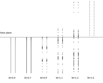
The governing equation involves two parameters W and D. Keeping D=0.1 fixed and increasing W leads to the sequence shown on Figure 2 after the release of 1000 vortex pairs and using N =20 substeps. In each figure a thick solid line shows the location of the rotor plane and we mark the location of each vortex, even though the left-hand column of vortices are simply mirror images of the right hand column. From left to right we firstly have W =0.0

modelling the hover state. Increasing the descent speed to W =0.7 gives the second picture in which the vortices still descend regularly, but whose spacing is reduced. The next three pictures show results for W =0.9, W =1.1 and W =1.3, all of which are unsteady and are classed as being in the vortex ring state. The vortices ejected downwards below the rotor plane are clustered together. At W =0.9 all the vortices move downwards, while at W =1.1

and W =1.3 some vortices escape upwards. The last image is for W =1.5 where we see that the windmill brake state has been reached, in which all vortices move upwards relative to the rotor in an organised manner. The pattern continues for all higher descent velocities, with the only change being that the vortex spacing increases.

Time traces for the same values of W are shown on figure 3, where we plot the time history of

t

w, the total velocity at the wing tip (z=0, y=0.5). Note that to better distinguish the curves

the dimensionless descent velocity has been added in each case. For D=0.1, unsteady results

vortex ring state cases all exhibit periodic or quasi-periodic variation of tip induced velocity. The signal at W =0.9 is periodic, while the higher two cases show evidence for subharmonic activity, although there is clearly a dominant frequency in each case. Chaotic motion was not seen for any value of W.

The basic mechanism for the cyclic variation is the steady build-up of circulation above the rotor plane, fed by new vortices with each rotor passage. This is illustrated clearly on Figure 4 which shows trajectories of all vortices up to n=250for a case W =1.1 and D=0.1. Approximately the first 50 vortices that are released are lost upwards relative to the rotor. However as the total circulation in the system increases as more vortices are released, there is eventually (by about n=70) enough self-induced downward motion to prevent vortices moving upwards and they accumulate near the rotor plane. Eventually the circulation near the rotor plane builds to a sufficient strength for the vortex to begin moving downwards under its self-induced velocity. It continues to accumulate new vortices, and hence accelerates

downwards, eventually being ejected from the rotor plane. After this release of circulation, new vortices then start to travel slowly upwards above the rotor plane typically extending up to 25% of span above the rotor plane, and the cycle repeats. At this value of W there are

occasionally vortices which escape upwards during the cycle. It can be seen that the release of vortex agglomerations downwards is quasi-periodic, with an ejection velocity such that they cover one wing span in about five vortex releases, with this velocity increasing with increasing D.

To study parametric influences, calculations have been run with up to 2500 vortex pairs for

0.01

D= (with n=2500and N =2), D=0.1 (with n=1000and N =20) and D=1.0(with

400

n= and N =200) with appropriate scalings chosen to best collapse the data. The effect of the numerical parameter N is discussed later. The amplitude of the oscillations is measured

as the peak-to-peak induced velocity variation w_p, averaged over 20 periods (note that fewer vortices are required at high values of D since the periods are short. A normalized amplitude

is defined as

* *

* p

p

w _T

A w

D

= =

Γ . (7)

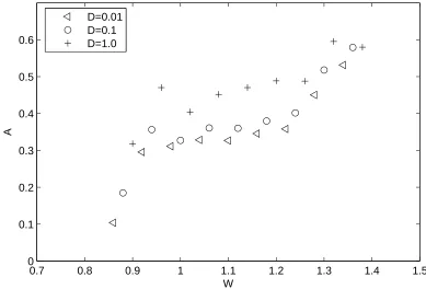
The amplitude variation over the unsteady range of descent parameter W is shown on Figure

5. The unsteady range is similar for all D. Amplitudes are small as the lower threshold of W is

crossed. A plateau is seen for0.95<W <1.2, before a further rise towards W =1.4, after which the windmill brake state is found. It should be noted that all these calculations start from a clean initial condition with no vortices in the flow. For these conditions W >1.4

always leads to a clean windmill state. In a helicopter configuration without forward flight, this upper boundary will be hysteretic: approaching it from below (helicopter accelerating downwards) will lead to the helicopter overtaking its previously-shed tip vortices, leading to unsteadiness well above this threshold. Approaching it from above (helicopter decelerating from a windmill state) will lead to a sudden onset of the unsteadiness.

The unsteadiness is harmonic in nature and the dominant frequency, f, can be easily extracted

from the signal. A non-dimensional frequency (or Strouhal number, St) which collapses the data is

* * * *

* St Wf W f b T

D

= =

This is plotted on figure 6; a typical Strouhal number St =0.136 0.017± is seen over the full range of unsteady values of W, with little dependence on the parameter D. The obvious alternative definition of a dimensionless frequency St= f D appears less relevant. The change from a stable to a periodic state as a single parameter (W in this case) is varied may often be characterized as a Hopf bifurcation. Figure 7 shows the amplitude variation near the onset of the periodic state. The amplitude data for D=0.1 fit a square root behaviourA=1.06 A−0.8545, confirming that this is indeed an example of a Hopf bifurcation.

The only numerical parameter in the problem is the number of substeps per introduction of a new vortex pair. For large numbers of substeps there is convergence for all cases. For the results shown previously we have taken N =2, 20, 200 for D=0.01, 0.1,1.0 respectively. Increasing N in proportion to D keeps the effective local timestep the same in each case. Table 1 shows some comparisons of amplitude and Strouhal number for halving and doubling the number of substeps at D=0.1. With N =20 and averaging over 20 periods, Strouhal numbers have typically converged to better than 1% and amplitudes to better than 2%. Table 1. Effect of number of substeps N on amplitude A and Strouhal number St at D=0.1,

1.0

W = .

N A St

10 0.3247 0.1473

20 0.3271 0.1465

40 0.3264 0.1465

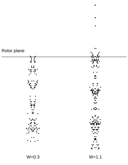
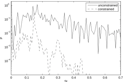
An unconstrained model was given in Section 2, in which the vortices are allowed to move in the y-z plane according to normal vortex dynamics, with a vortex core parameter ε. Examples of unconstrained computations with ε =0.01 and D=0.1 are shown on Figure 8 for two descent velocities W =0.3 (left hand plot) and W =1.1 (right hand plot). In each case the number of substeps was chosen as N =20. In each case the flow is more chaotic than in the constrained problem. At W =0.3 we can see that the initial motion of the vortices is smooth but the wake becomes unstable and chaotic quite quickly. Since this instability occurs away from the rotor plane the variations of tip induced velocity are small, withA≈0.006. At the higher descent velocity of W =1.1 this amplitude increases toA≈0.2. The flow is chaotic, but the instantaneous picture does provide some indication that large agglomerations of vortices are being shed downwards. A power spectrum of the tip velocity at W =1.1 is shown on Figure 9, comparing the constrained and unconstrained cases. In the constrained model there is evidence for first and second harmonics as well as the first subharmonic. For the constrained model the spectrum is broadband with a maximum atSt=0.167, which is close to the peak for the constrained model. This indicates that the constrained model is useful for extracting the mechanism of the dominant model from the otherwise noisy signal from the unconstrained model.

4. Discussion

The unconstrained model given at the end of Section 2 can be classed as a standard vortex dynamics treatment of the plane problem of a wing descending into the wake vortices of a succession of aircraft. Results from this model are complex, even in two dimensions, as shown in the previous section. The attraction of the constrained model is its simplicity and ability to demonstrate the key underlying dynamics, for example the periodic state of

shedding of vortex agglomerations, which are otherwise buried in a complex time signal. The succession of flow states that emerge from the constrained model with increasing descent velocity, namely hover state, Hopf bifurcation to periodic shedding, and hysteretic transition to the windmill state, provide a different perspective on the vortex ring state seen in

helicopter flight, emphasising unsteady aspects of the problem.

An even simpler discrete algorithm may be derived if we consider explicit Euler time

advance and choose N =1. This simplified treatment still exhibits the main physical features presented in the previous section. Although numerical integration errors are now inseparable from the physical response, the quantitative effect of this is small for D<0.1. Pseudo code for this case is given in Figure 10, illustrating the simplicity of the algorithm. Experience has shown that animations are the best way to visualize the response.

A connection to standard helicopter terminology is possible if we take the rotor radius *

R to be _b*_{/ 2. The time between tip vortex injections is} *

(

)

2 _b

T = π N Ω , where _Ω*

is the angular rotation rate (rad/s) and N is the number of blades. Assuming a constant circulation _b

(Leishman [2] Section 3.3) we have *2 *

* 2 T

b

R C

N

π Ω

Γ = (9)

where *

(

)

T Z

C =F ρ πR Ω is a thrust coefficient based on the vertical force * Z

F ). Hence we can connect the parameter D with a helicopter thrust coefficient by

2 2 T b D C N π = (10)

With a typical values of 0.01<C_T <0.05 and two blades (for equivalence with the planar wing model) we have 0.025< <D 0.123, which is within the range of values for which results have been given in the previous section.

The descent velocity, normalised by the hover-induced downwash is defined by *

* h

W w

µ= , (11)

with the hover-induced velocity given by * * *

2

T h

C

w = Ω R . (12)

With a little rearrangement we have

2

W

µ= (13)

Two corrections are needed to make a direct comparison with helicopter results. Firstly, the induced velocity constant 1 2πin (2) for planar vortices needs to be changed for

Secondly, account needs to be taken of the change in aerodynamic effectiveness of the rotor; for example a factor of three reduction in thrust coefficient (and hence the model circulation

*

Γ ) was seen by Stack et al. [6]. The combination of effects with the magnitudes given (approximately a factor of two increase for axisymmetric rings and factor of three reduction in aerodynamic efficiency) would be a slight reduction (by a factor of 1.5 ) in the predicted

c

µ for VRS onset, down toµ_c =0.98. This compares with µ_c =0.6to µ_c =0.7 seen by Leishman et al [2,4] and µ_c=1.05 seen by Stack et al. We note that the aerodynamic efficiency effect is large, and could be included via a blade element model, with associated assumptions about the low Reynolds number and stalling behaviour of rotor blades. The detail of such a refinement necessarily involves additional empiricism; the main point to note is that the predicted values ofµ_cfrom the simple constrained model are of similar order to the experimental data, indicating that the right physical phenomena have been captured.

Finally, it is noted that simple momentum theory is valid for the windmill brake state for µ >2 [2]. Using (13), this is equivalent toW > 2, which is thus in close correspondence with the numerical result W >1.40.

5. Conclusions

It has been shown how a simple vortex model with constrained motion is capable of reproducing some physical phenomena associated with the descent of a rotorcraft. At a critical descent speed there is a Hopf bifurcation from a steady hover state into a periodic solution. The mechanism involves a steady build-up of circulation above the rotor plane followed by ejection downwards of large agglomerations of vortices. A Strouhal number is defined and is shown to be able to collapse the frequency data. At high values of descent velocity there is a return to a windmill brake state where all vortices travel upwards relative to the rotor. The model offers a rational basis for predicting the onset of vortex ring state and identifies some important physics contained within a more complex line vortex and vortex filament simulations, but hidden by the presence of other complexities such as wake roll-up of vortices.

Acknowledgements

The author would like to thank Dr Simon Newman for checking some of the calculation results and Dr Karim Shariff of NASA-Ames for suggesting the comparison with unconstrained vortex simulations.

References

[1] Brown, R.E., Leishman, J.G., Newman, S.J. and Perry, F.J. 2002 Blade twist effects on rotor behaviour in the vortex ring state. European Rotorcraft Forum, Sept 17-20, Bristol, UK.

[2] Leishman, J.G. 2000 Principles of Helicopter Aerodynamics. Cambridge University Press.

[4] Leishman, J.G., Bhagwat, M.J. and Ananthan, S. 2004 The vortex ring state as a spatially and temporally developing wake instability. J. American Helicopter Society 49(2), 160-175.

[5] Newman, S., Brown, R., Perry, J. Lewis, S, Orchard, M and Modha, A. 2003 Predicting the onset of wake breakdown for rotors in descending flight. J. American Helicopter Society 48(1), 28-38.

Γ

*

b

y

*

ij

r

Rotor plane

i’th

vortex

j’th

vortex

z

Figure 1. Schematic of the vortex arrangement in hover or slow descent.

W=0.0 W=0.7 W=0.9 W=1.1 W=1.3 W=1.5

Rotor plane

0 100 200 300 400 500 600 700 800 900 1000 −0.5

0 0.5 1 1.5 2

n

w t

+W

W=0.0 W=0.7 W=0.9 W=1.1 W=1.3 W=1.5

Figure 3.Time variation of tip induced velocity w , covering the rage of descent velocities _t

from hover (W =0.0) to windmill brake state (W =1.5). For clarity the curves are shifted by plotting w_t+W.

0 50 100 150 200 250

−5 −4 −3 −2 −1 0 1 2 3 4 5

n

z

0.7 0.8 0.9 1 1.1 1.2 1.3 1.4 1.5 0

0.1 0.2 0.3 0.4 0.5 0.6

W

A

D=0.01 D=0.1 D=1.0

Figure 5. Normalised peak-to-peak amplitude w_p as a function of normalised descent velocity for loading parameter values D=0.01, 0.1 and 1.0

0.7 0.8 0.9 1 1.1 1.2 1.3 1.4 1.5

0 0.02 0.04 0.06 0.08 0.1 0.12 0.14 0.16 0.18 0.2

W

St

D=0.01 D=0.1 D=1.0

0.840 0.845 0.85 0.855 0.86 0.865 0.87 0.875 0.88 0.885 0.89 0.02

0.04 0.06 0.08 0.1 0.12 0.14 0.16 0.18 0.2

W

A

1.08(W−0.8545)0.5 Model

Figure 7. Amplitude variation near the onset of oscillations, with the square root behaviour confirming the presence of a Hopf bifurcation.

W=0.3 W=1.1

Rotor plane

0 0.1 0.2 0.3 0.4 0.5 0.6 0.7 10−4

10−3 10−2 10−1 100

St

P

unconstrained constrained

Figure 9. Spectrum of tip induced velocity from constrained (dashed line) and unconstrained (solid line) model at W=1.1, D=0.1.

for n=1:nmax z(n)=0. for i=1:n

w(i)=0. for j=1:n

w(i)=w(i)-1./(1.+(z(i)-z(j))^2) end

end

for i=1:n

z(i)=z(i)+W*sqrt(D)+D*w(i)/(2.*pi) end

end