Low Complexity Non-Binary LDPC and Modulation Schemes Communicating over MIMO
Channels
Feng Guo and Lajos Hanzo
1School of ECS, University of Southampton, SO17 1BJ, UK.
Tel: +44-23-8059-3125, Fax: +44-23-8059-4508
Email:lh
1@ecs.soton.ac.uk
,
http://www-mobile.ecs.soton.ac.uk
Abstract–In this contribution, Pearl’sbelief propagation(BP) algorithm is invoked for constructing a belief network, which is employed for developing a joint detection aided transmit diver-sity scheme and a non-binary LDPC decoder constructed over
a finite field of GF(q). An exciting bit-by-bit detection scheme
is further developed for creating the joint purly symbol-based LDPC/transmit diversity decoder. The performance of the pro-posed symbol-based system is benchmarked against the original bit-by-bit detection scheme, when communicating over an uncor-related Rayleigh fading channel using two transmitters and two receivers. The associated detection complexities are also com-pared .
1. INTRODUCTION AND SYSTEM SCHEMATIC
1.1. Motivation and State-of-the-Art
Since the invention of turbo codes by Berrou [1]et. al, the superior performance of iterative decoders has attracted substantial research interest. The family of Low Density Parity Check (LDPC) codes originally devised by Gallager as early as 1963 [2] has also been ex-tensively studied during the 1990s [3, 4]. More recently, Mackay, McEliece and Cheng [5] pointed out that Gallager’sprobabilistic LDP C decodingalgorithm [6], constitutes an instance of Pearl’s be-lief propagation algorithm. Mackay and Neal demonstrated in [7] that despite their simple decoding structure, LDPC codes are also capa-ble of operating near the channel capacity. Richardson [8] suggested the employment of a differential belief propagation decoding algo-rithm for binary LDPC codes using the Fast Fourier Transform (FFT) for reducing the decoding complexity imposed. In 1998, Davey and Mackay proposed a non-binary version of LDPC codes [9], which was potentially capable of outperforming binary LDPC codes. When using Richardson’s FFT-based decoding algorithm [8], the complex-ity of non-binary LDPCs increases only linearly with respect to the size of the associated Galois field.
These non-binary LDPC codes may be conveniently combined with multilevel modulation and/or multiple antenna schemes, which are capable of supporting high data rate transmissions [10]. In this contribution, an LDPC-coded low-complexity transmitter and two-receiver scheme will be studied.
This contribution is structured as follows. In Section 2, a brief overview of Baysian networks [11] and Pearl’sbelief propagation
algorithm [11] will be given. Section 3 introduces non-binary LDPC decoding over GF(q). Section 4 details the symbol-by-symbol joint detection algorithm advocated. Section 5 characterises the achiev-able performance of the proposed system in contrast to the corre-sponding bit-by-bit detection scheme proposed by Meshkat and Ja-farkhani [12]. The proposed system will be characterized using 4QAM,
The financial support of the Mobile VCE, UK; EPSRC, UK and that of the European Union is gratefully ackowledged.
8PSK and 16QAM transmission schemes having a throughput of 2, 3 and 4 bits per symbol (BPS). Finally, Section 6 will provide a com-plexity comparison, while Section 7 offers our conclusions.
1.2. System Schematic
The overall system schematic is illustrated in Figure 1. The source bits are encoded by a non-binary LDPC encoder, and the LDPC en-coded symbols are mapped to the corresponding QAM symbols, which are transmitted by the multiple antenna based transmit diversity sys-tem. The channel’s output signalris then fed into the demodulator where the soft-metricMr−>v(sk)is calculated. More explicitly, the notation
Mr−>v(sk)represents the soft metric passed from the demodulator
to the LDPC decoder based on the symbol probability of thekth de-coded symbol of the LDPC de-codedword. As seen in Figure 1, these soft-metrics are passed to the LDPC decoder, which carries out an LDPC iteration and produces the resultanta posteriori probability Ppost. Based on thea posteriori probability, a tentative hard
de-cision will be made and the resultant codeword will be check by the LPDC code’s parity check matrix. If the resultant vector is an all-zero sequence, then a legitimate codeword has been found, and the hard-decision based sequence will be output. Otherwise, if the max-imum number of iterations has not been reached, thea posteriori probabilitywill be subtracted from the original soft metric denoted byMr−>v(sk)and fed back to the demodulator for the next
itera-tion, as seen in Figure 1. This process continues until the pre-defined maximum number of iterations has been encountered or a legitimate codeword has been found.
+
Mr−>v
Mr−>v
Source LDPC Mapper
Tx / Rx
LDPC Decoder Max
Iteration Reached?
Y Y
Output N
Bits Encoder
r Encoded
Symbols
−
Multiple Antenna
Valid codeword
?
DeModulation
[image:1.595.315.535.545.678.2]Ppost
2. BAYSIAN NETWORKS AND BELIEF PROPAGATION
In this section, we provide a rudimentary introduction to both Baysian networks [11] and to the classic belief propagation algorithm [11].
X1
X2
X3
X4
X5
[image:2.595.87.256.106.224.2]X6
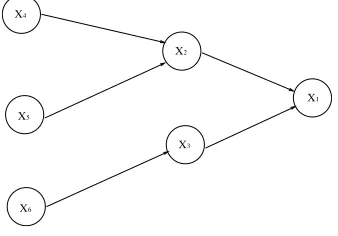
Figure 2: Baysian network having six nodes
Let us illustrate the associated concepts with the aid of an ex-ample. In Figure 2, we assume that X4, X5 andX6 are the
so-called evidence or observation nodes and we would like to infer the
a posteriori probability ofX1. Hence by assuming thatP(X4),
P(X5)as well asP(X6)are known and given that the relationship of the various variables is characterized by the directed links seen in Figure 2, thea posterioriprobability ofX1 can be represented as follows:
P(X1) =P(X1|X2, X3)·P(X2|X4, X5)·P(X3|X6)
·P(X4)·P(X5)·P(X6). (1) If we use the notationPp(Xi)for representing the parent node set of nodei, Equation 1 may be rewritten as:
P(X1) = N
i=1
P(xi|Pp(xi)). (2)
In general a Baysian network consists of a set of random variables denoted byX={X1, X2...Xn}and these random variables are rep-resented by the nodes of the network. Between the nodes, there are di-rected links representing the relationship of the so-calledparent nodes
with the so-calledchild nodes. Some of the nodes may correspond to random variables, whose values are encountered and hence observed, which are the previously mentioned ”evidence nodes” or ”observa-tion nodes” [12]. When a specific set of variables corresponding to the evidence nodes is observed, the belief propagation algorithm may be invoked for inferring thea posterioriinformation corresponding to the rest of the nodes in the network, as it was demonstrated in the context of Figure 2.
Since LDPC codes may be conveniently characterized by the vari-able nodes, check nodes and their inter-connections [13], a corre-sponding Baysian network can be constructed. Furthermore, in this contribution, the multiple antenna aided transmit diversity scheme may also be represented as a Baysian network. Hence Section 4 will detail the process of developing a tri-partite Baysian network for the system proposed where the associated belief propagation algorithm invoked for this tri-partite Baysian network will also be described.
3. NON BINARY LDPC
Gallager’s original binary LDPC codes are defined by a sparse parity check matrix (PCM) having a relatively low fraction of non-zero par-ity check entries in the matrix. A codeword is a legitimate one, if its
product with the PCM using modulo-2 multiplications and additions is an all-zero vector. Davey and Mackay generalized the family of binary LDPC codes for a Galois Field of sizeq, i.e. for GF(q). These non-binary LDPC codes are defined by a similar sparse PCM, with the exception that the non-zero entries may now assume any integer value between1and(q−1). Thus the product of a legitimate code-word with the PCM calculated over GF(q) is an all zero vector, which is expressed as:
j∈N(m)
Hmj(xj) = 0,over GF(q), (3)
whereN(m)is a set containing all the column indices of the non-zero entries in themthrow, and the variableHmjrepresents the value of the non-zero entry in themthrow andjthcolumn of the PCM, which ranges from1to(q−1). Furthermore,xj represents the surviving
state of thejthsymbol of the codeword, which is defined as the sym-bol state having the highesta posteriori probability among theq
number of legitimate states. Since the non-zero entries in the PCM are elements of GF(q), they may also be represented as binary strings constituted bypbits, where2p=q. In Equation 3 the variablexjalso assumes values ranging from0toq−1, thus it may be represented by a binary bit string of sizep=log2q. It has been shown [14] that
anM×Nnon-binary PCM constructed over GF(q) has an equiva-lent binary PCM of sizeM p×N p[14]. It has been shown in [15] that LDPC codes have to have a high column weight for the sake of achieving a good performance. However, a high column weight will introduce more short cycles in the PCM and this in turn degrades the achievable performance. The advantage of using non-binary LDPC codes is that the equivalent binary weight of the PCM is increased, while the number of short cycles may remain low [14].
As in binary LDPC codes, the non-zero entries of the PCM it-eratively update the quantitiesRamn andQamn, whereRamn repre-sents the probability of themthcheck being satisfied, when symbol
nof the codeword is considered to be in statea ∈GF(q)and the other symbols have a separable distribution given by the probabilities
{Qbmn :n∈ N(m)\n, b∈GF(q)}. The calculation of probability Ramnis formulated as :
Ram,n=
x:xn=b
P(zm= 0|x)
k∈N(m),k=n Qxk
mk. (4)
More explicitly, this implies that the quantityRamn represents the
Probability Density Function (PDF) of thenthsymbol being in any of theqnumber of legitimate states, given the knowledge of each indi-vidual PDF for the rest of the symbols participating in themthcheck, and given that themthcheck is satisfied.
Furthermore, the quantityQamndenotes the probability of thenth
symbol being in the statea∈GF(q)calculated from the probabilities
{Ramn:m∈ M(n)\m}according to:
Qam,n=αm,nfna
k∈M(n),k=m
Rak,n. (5)
More explicitly, the quantityQamnis given by multiplying theintrinsic probability fnaby the product of probabilitiesRamnprovided by all check nodes except themth, indicating that thenthsymbol is in state
a. HereN(i)andM(i)represented a set of column and row indices of the non-zero entries in theithrow and column of the PCM, respec-tively. The quantityRamnandQamnare updated as follows.
After each iteration, thea posterioriprobabilityPnawill be cal-culated based on theintrinsic probability fnaof thenthreceived
sample and on the information updated as well as delivered byRamn
Pna=αnfna
k∈M(n)
Rak,n. (6)
The quantityαin Equations 5 and 6 represents a normalization factor required for ensuring that the conditionsa∈GF(q)Qamn= 1
anda∈GF(q)Pna= 1are satisfied. In Equation 4, the termP(zm= 0|x)is acting as a binary flag, which returns a value of 1, if the current codewordxsatisfies themthcheck, or 0 otherwise. More explicitly, this expression has to be evaluated for all legitimate manifestations of the codewordx, which becomes computationally prohibitive, when the blocklength is high. However, since the operation of updating the quantityRamnin Equation 4 corresponds to calculating the joint
probability of all symbols withinN(m)over GF(q) given in the form of the corresponding sum multiplied by their corresponding matrix entry, i.e. by the probability of
P(
x:xn=b
xn·Hmn=a), a∈GF(q), (7)
thus a multi-dimensional FFT [14] over GF(q) may be invoked for the sake of reducing the complexity imposed.
4. JOINT DETECTION SYSTEM
In this section, we will invoke the Baysian network of Section 2 for characterising the LDPC decoder amalgamated with a transmit diver-sity scheme originally proposed by Meshkat and Jafarkhani, which was detected using a bit-by-bit decoding algorithm [12].
c
[image:3.595.341.506.358.557.2]r v
Figure 3: Tri-partite graph of the jointly detected transmit diversity system using LDPC coding
In Figure 3 the squares represent the check nodes of the LDPC code, while the circles correspond to its variable nodes. The black dots represents the channel outputs. The connections between the squares and the circles represent the non-zero entries within the PCM. After the LDPC encoding process, each variable node contains an en-coded LDPC symbol constituted byp = log2qbits. Each pair of symbols is transmitted by the two transmitters and received by the two receiver antennas through four propagation paths. Thus the lines connecting the circles and black dots represent the two-transmitter, two-receiver system. In the butterfly-shaped section of Figure 3 each pair of the channel outputs is correlated, since they originate from the same pair of modulated symbols, which are transmitted through four different propagation paths by the two-antenna system. The message passing scheme of the joint decoder may be described as follows. In the associated equations, we will user,vandcfor representing the received channel output, the variable nodes and the check nodes, re-spectively.
Following the approach of [12], initially thejthsoft channel out-put is passed from the black dots in Figure 3 to the variable nodes
(circles) of the LDPC decoder and the associated confidence mea-sures are calculated by comparing the soft channel output values to all legitimate transmitted symbols according to [12] :
Mr−>v(bk) = all Bi
1 (√2πσn)nre
−|r−HS(2Bi,bkσ2n )|2 ·
bj∈Bi
Mv−>r(bj). (8)
In Equation 8,σnrepresents the standard deviation of the Gaus-sian noise,His annr×ntmatrix containing the complex valued fading coefficients of each transmission path, wherenr andnt are the number of receiver and transmitter antennas, respectively. Using
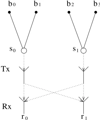
bpsrepresenting the number of bits per symbol for the correspond-ing modulation scheme, Bi represents the set of(nt ×bps)−1
transmitted bits, but excludes thekthbitbk, which contributes to the value of the received vectorrat thenr number of receivers, while S(Bi, bk)is a vector ofntcomponents containing the symbols corre-sponding to the bit set ofBiandbk. More explicitly, let us consider Figure 4, for example. When using QPSK modulation, four bits are mapped into two QPSK symbols and transmitted by the two trans-mitters to the two receivers. IfMr−>v(b2)is under consideration, then we haveBi={b0, b1, b3}and(Bi, b2) ={b0, b1, b2, b3}. The vectorrwill contain elements of {r0, r1}. For a particular set of
Bi = {b0 = 1, b1 = 1, b3 = 0}, since QPSK modulation is em-ployed in Figure 4, thus the notationS(Bi, b2)represents{11,00}or
{11,10}, depending on the specific value ofb2concerned.
r
0r
1b
Tx
Rx
b
b
b
s
s
0
0 1
1 2 3
Figure 4: Schematic of a two-transmitter two-receiver system using QPSK modulation
The metricMr−>v(bk)is then passed to the variable nodes, and the following message is calculated at the variable nodes [12]:
Mvk−>ci(bk) =αkMr−>v(bk)
j∈M(k),j=i
Mcj−>vk(bk), (9)
which is then passed onto the check nodes. The structure of Equation 9 is similar to the update formula ofQamnseen in Equation 5, with
the exception that the constantintrinsicinformationfnain Equation
[image:3.595.86.254.364.468.2]The metricMcj−>vk(bk)of Equation 9 corresponds toRaknin
Equation 5, which is then passed from the check nodes to the vari-able nodes, and updated according to Equation 4. Then the message
Mv−>r(bk)has to be passed from the variable node back to the
chan-nel output, which is formulated as:
Mv−>r(bk) =α
j∈M(k)
Mcj−>vk(bk). (10)
This operation is similar to Equation 6, however theinstrinsic informationfnaseen in Equation 6 is omitted from Equation 10 and
the metricMv−>r(bk)is fed back to the channel output nodes from the variable nodes. More explicitly, the reason that theintrinsic inf ormation is omitted in this case is, because this information, which was denoted byMr−>v(bk)in Equation 9 has been used
dur-ing the calculation of the metric Mvk−>ci(bk)and thus it should be excluded, when providingextrinsicinformation for the channel output nodes.
Again, the above-mentioned procedure was proposed by Meshkat and Jafarkhani in [12] for a binary system. In Equation 8, the a priori inf ormationis calculated on a bit-by-bit basis, assuming that the bits are independent of each other. However, this assump-tion is only approximatly valid in Gray-coded non-binary modulaassump-tion schemes. Hence it is beneficial to combine non-binary QAM schemes with matching non-binary LDPC codes, since this process requires no symbol to bit probability conversion. Furthermore, we will show in Section 6 that upon using a purly symbol based joint decoding tech-nique, the associated decoding complexity may be significantly re-duced. Hence the bit-by-bit based metric update formula of Equation 8 is converted to its symbol-based counterpart as:
Mr−>v(sk) = all Si
1 (√2πσn)nre
−|r−HS(2Si,skσ2n )|2 ·
sj∈Si
Mv−>r(sj). (11)
In Equation 11,Sinow represents a set of(nt−1)number of
symbols rather than(nt×bps−1)number of bits, including all
sym-bols, except forsk, which contributes to the value of the received vectorrat thenrreceivers, andS(Si, sk)is a vector of sizent con-taining the symbols includings0 ands1, as in Figure 4. More ex-plicitly, rather than using the bits representing the symbols in Figure 4 for the calculation of thea priori inf ormation, the symbols are employed directly in this scheme. Hence, if symbols1of Figure 4 is
concerned, the vectorSiwill have only one element of{s0}. Thea priori inf ormationMv−>r(sj)represents the probability of the
jthsymbol, rather than that of the bits in Equation 8.
5. SIMULATION RESULTS
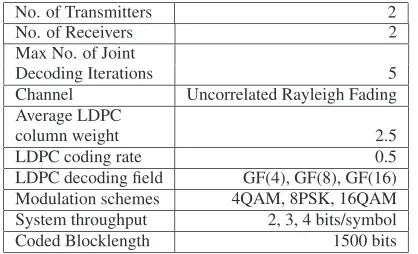
In this section, the achievable performance of the proposed system is characterized. All simulation parameters are listed in Table 1. We used 4QAM, 8PSK and 16QAM transmission for the sake of increas-ing the throughput of the system. Correspondincreas-ingly, non-binary LDPC codes operating over GF(4), GF(8) and GF(16) were used. Since the number of transmitters was set to two and the LDPC code had a cod-ing rate of 1/2, the effective throughput was 2, 3 and 4 bits/symbol, for the corresponding configurations. More explicitly, the effective throughput of the modems was not reduced by the 1/2-rate LDPC codec, because the doubled number of bits was conveyed by two transmit antennas. A coded blocklength of 1500 bits was used.
No. of Transmitters 2
No. of Receivers 2
Max No. of Joint
Decoding Iterations 5
Channel Uncorrelated Rayleigh Fading
Average LDPC
column weight 2.5
LDPC coding rate 0.5
LDPC decoding field GF(4), GF(8), GF(16)
Modulation schemes 4QAM, 8PSK, 16QAM
System throughput 2, 3, 4 bits/symbol
[image:4.595.322.531.56.183.2]Coded Blocklength 1500 bits
Table 1: System simulation parameters
0 1 2 3 4 5 6 7 8 9 10
E
b/N
0(dB)
10-5
2 5
10-4
2 5
10-3
2 5
10-2
2 5
10-1
2 5
100
BER
16QAM 8PSK 4QAM
[image:4.595.324.540.237.413.2]Bit-based + binary LDPC Symbol-based + non-binary LDPC
Figure 5: Performance of the symbol-based joint decoding aided sys-tem using non-binary LDPC codes for communicating over uncor-related Rayleigh fading channels. The performance of the bit-based joint decoding system of [12] using a 1/2-rate binary LDPC code was also plotted as a benchmarker.
In Figure 5 it may be observed that by using the proposed symbol based joint decoding algorithm, a better bit error ratio (BER) perfor-mance is achieved than that of the original bit-based algorithm. An approximately 2dB gain was achieved at a BER of10−5for all of the three modulation schemes used.
6. COMPLEXITY
In this section the complexity of the proposed system is estimated. When the number of bits per symbol is increased, calculating thea priori probabilityusing the bit-by-bit approach of Equation 8 will become quite complex. Using non-binary LDPCs will also increase the decoding complexity, however, this increase is only linearly de-pendent on the number of bits, if the multi-dimensional FFT based LDPC decoder of [14] is used.
As seen from Equation 8, the decoding operations require the evaluation of all possible input symbol configurations containing the
* Bit-based Symbol-based
4QAM 179 91
8PSK 739 198
16QAM 3338 518
+ Bit-based Symbol-based
4QAM 27 28
8PSK 75 61
[image:5.595.98.245.55.140.2]16QAM 267 144
Table 2: Complexity comparison between the bit-based benchmarker algorithm of [12] and the proposed symbol-based algorithm using the simulation parameters listed in Table 1.
2 4 6 8 10 12 14 16 18 No. of Modulation levels 0
50 100 150 200 250 300 350 400 450 500
Number
of
Operations
Additions
Symbol based Bit based
2 4 6 8 10 12 14 16 18 No. of Modulation levels 0
500 1000 1500 2000 2500 3000 3500 4000 4500 5000
Number
of
Operations
Multiplications
Symbol based Bit based
Figure 6: Complexity comparison between the bit-based benchmarker algorithm of [12] and the proposed symbol-based algorithm using the simulation parameters listed in Table 1.
system havingnttransmitters andbpsnumber of bits per symbol, the total number of metric evaluations using Equation 8 will be2bps·nr. Each metric evaluation requiresnt×nrnumber of multiplications for determiningHS(Bi, bk)in Equation 8, one multiplication for
evalu-ating the square, and one for carrying out the required division. One substraction is needed for finding the Euclidean distance between the received sample and each of the constellation points. Furthermore, for each metric evaluation,bps×nt−1number of multiplications are needed for calculating thea priori probability. Thus, for each decoded bit, the required number of multiplications becomes((bps× nt−1)+(nt×nr+2))×2bps×nt= (nt×(bps+nr)+1)×2bps×nt.
The required number of additions is 2bps×nt. By contrast, for the proposed non-binary system using Equation 11, the number of multi-plications needed for thea priori probabilitycalculation is reduced to(nt−1), since we are directly determining the symbol probabil-ity. Thus the overall number of multiplications per bit for the symbol based system is(nt×(nr+ 1) + 1)×2bps×nt/bpsand the number
of additions is2bps×nt/bpsper bit.
On the other hand, upon employing non-binary LDPC codes, the message passing between the system components becomes more com-plex owing to the increased GF size. The number of multiplications and additions required for each decoding bit can be represented as
7tq/log2(q)and2tq, wheretandq are the LDPC code’s average column weight and GF size, respectively [14]. Hence the overall complexity required by the two systems in each of the modulation schemes is listed in Table 2, and plotted in Figure 6.
From Table 2 and Figure 6, it can be observed that by using the proposed symbol-by-symbol joint decoding algorithm, the complex-ity may be significantly reduced. For example, in case of 16QAM, a complexity reduction in excess of 80 percent was achieved. This complexity reduction becomes even higher for 64QAM. For the sake of simplicity in this comparison, the complexity increase imposed by the extra finite field multiplication during the codeword validation was ignored.
7. CONCLUSION
In this contribution, a novel symbol based joint detection algorithm was proposed for non-binary LDPC-coded transmit diversity-aided transmissions. The proposed purely symbol-based system was ca-pable of achieving a gain of approximately 2dB for QPSK, 8PSK and 16QAM transmissions in comparison to the identical-throughput bit-by-bit benchmarker algorithm. The scheme advocated was also shown to be less compolex than its binary benchmarker.
8. REFERENCES
[1] C. Berrou, A. Glavieux and P. Thitimajshima, “Near Shannon Limit Error-Correcting Coding and Decoding : Turbo Codes,” in Proceed-ings of the IEEE International Confrence on Communications, pp. 1064– 1070, 1993.
[2] R. Gallager, “Low Density Parity Check Codes,”IEEE Transaction on Information Theory, vol. 8, pp. 21–28, Jan. 1962.
[3] S. T. Brink, G. Framer, A. Ashikhmin, “Design of low-density parity-check codes for modulation and detection,”IEEE Transaction on Com-munications, vol. 52, pp. 670–678, April 2004.
[4] B. Lu, G Yue and X. Wang, “Performance analysis and design optimiza-tion of LDPC-coded MIMO OFDM systems,”IEEE Transaction on Sig-nal Processing, vol. 52, pp. 348 – 361, Feb. 2004.
[5] R. J. McEliece, D. J. C. MacKay, J. F. Cheng, “Turbo Decoding as an Instance of Pearl’s Belief Propagation Algorithm,”IEEE Journal on Se-lected Areas in Communications, vol. 16, pp. 140–152, Feb. 1998.
[6] R. Gallager, “Low Density Parity Check Codes,”Ph.D thesis,M.I.T,USA, 1963.
[7] D. J. C MacKay, and R. M. Neal, “Near Shannon Limit Performance of Low Density Parity Check Codes,”Electronics Letters, vol. 33, pp. 457– 458, 13 March 1997.
[8] T. Richardson, R. Urbanke, “The Capacity of Low-Density Parity Check Codes Under Message-Passing Decoding,”IEEE Transaction on Infor-mation Theory, vol. 47, pp. 599–618, Feb. 2001.
[9] M. C. Davey and D. J. C MacKay, “Low Density Parity Check Codes over GF(q),”IEEE Communications Letters, vol. 2, pp. 165–167, June 1998.
[10] L. Hanzo, T. H. Liew, B. L. Yeap, S. X. Ng,Turbo Coding, Turbo Equal-isation and Space-Time Coding for transmission over fading channels, ch. 9, pp. 317–390. Wiley & IEEE, 2002.
[11] J. Pearl, “Probabilistic Reasoning in Intelligent Systems,”San Mateo, CA:Morgan Kaufmann, 1988.
[12] P. Meshkat and H. Jafarkhani, “Space-Time Low-Density Parity-Check Codes,” vol. 2, (Pacific Grove, Monterey, CA, USA), pp. 1117 –1121, 3-6, Nov 2002.
[13] M. R. Tanner, “A Recursive Approach to Low Complexity Codes,”IEEE Transactions on Information Theory, vol. 27, September 1981.
[14] M.C. Davey, “Error-Correction using Low Density Parity Check Codes,”
Ph.D thesis, University of Cambridge,UK, 1999.
[image:5.595.57.283.191.294.2]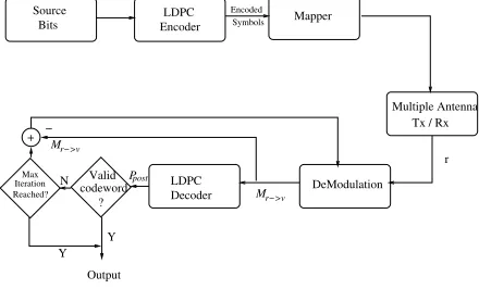
![Figure 6: Complexity comparison between the bit-based benchmarkeralgorithm of [12] and the proposed symbol-based algorithm using thesimulation parameters listed in Table 1.](https://thumb-us.123doks.com/thumbv2/123dok_us/8517883.352141/5.595.98.245.55.140/figure-complexity-comparison-benchmarkeralgorithm-proposed-algorithm-thesimulation-parameters.webp)
