Direct Methods for Solving the Schrödinger Equation

the Schrödinger Equation

Explicitly Correlated Wavefunctions

Mohammad Mostafanejad

Research School of Chemistry

College of Physical and Mathematical Sciences

A thesis submitted for the degree of

Master of Philosophy

of the Australian National University

November 2016

© Copyright by

I hereby declare that to my best knowledge, the contents of this thesis are original and

have not been submitted in whole or in part for consideration for any other degree or

qualifi-cation at ANU, or any other university. Also, necessary citations have been carefully and

explicitly made throughout the text whenever they referred to the work of other persons. This

dissertation contains fewer than 60,000 words excluding appendices, bibliography, footnotes,

tables, figures and equations.

Mohammad Mostafanejad

I would like to thank ANU for the IPRS scholarship. Inspiring and fruitful discussions with

our sabbatical visitors Prof. Patrick Bultinck from Ghent University which led to an

inter-esting project on the performance of the Hylleraas-configuration interaction wavefunction,

and Prof. Vitaly Rassolov from University of South Carolina which resulted in a deeper

understanding of mine about the electron correlation problem and correlation operators are

also acknowledged. I am indebted to our physicist visitor Prof. Nimrod Moiseyev for the

fascinating discussion about complex and stability analyses and sending me valuable papers

from his PhD project. I am also grateful to Dr. Andrew Thomas Beresford Gilbert for his

expertise in mathematics who was a great source of learning for me and Dr. Marat Sibaev for

The notions of electron correlation and correlation problem arising in the framework of

approximate solutions to the Schrödinger equation are presented. Then, we briefly review the

original ideas of explicit inclusion of the interelectronic distance,r₁₂, into the wavefunction

as a solution to this problem.

Exemplifying the efficiency of the explicit correlation for achieving high accuracy, we

analyze the Nakatsuji’s free-complement (FC) method. We demonstrate that at each FC

order, fewer number of complement functions is required to get lower energies compared

with those resulting from the conventional FC method. Applying the FC method to the triplet

excited state of the He atom, we have discovered the appearance of permanents in addition to

the determinants in the FC expansion of the wavefunction. These permanents are shown to

be important for the energy convergence.

To achieve a better understanding about the explicitly correlated methods, especially,

the R12 and F12 methods, we analyzed three possible candidates with various correlation

theory of the Frost and Braunstein (FB). We revisit CMO theory within both restricted (R)

and unrestricted formalisms (U). We also introduce the unrestricted FB (UFB) ansatz for

the first time and derive the necessary expressions for both RFB and UFB overlap, kinetic,

nuclear-attraction and interelectronic Coulomb repulsion matrix elements. All integrals have

been obtained in closed form except one for which, we have used an accurate one-dimensional

quadrature.

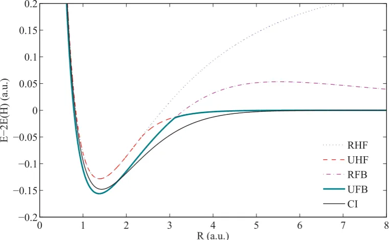
Finally, we investigate the potential energy curve (PEC) of UFB for H2at small,

inter-mediate and large internuclear distances. Then, we compare its performance with that of

RFB, restricted Hartree-Fock (RHF), unrestricted Hartree-Fock (UHF) and configuration

interaction (CI) wavefunctions. Reproducing the RFB results for a much wider range of

bond lengths in H2reveals that the calculations of FB contain significant errors. We have

also found a pole in the RFB linear correlation coefficient. Our UFB ansatz provides

signifi-cant improvement over the RFB where passing the symmetry breaking point it completely

removes the hump in the RFB PEC. The UFB ansatz also shows surprising features such

as the presence of multiple solutions, non-smooth PEC, symmetry-broken solutions that

are higher in energy than the restricted solution and RFB→UFB stability in the presence of lower UFB solutions. These phenomena can have significant impacts on the explicitly

correlated calculations such as R12 and F12 within the unrestricted framework. Also, a

detailed discussion on the large-Rasymptotic analysis of these five wavefunctions shows

that none of these PECs has the correctO(R−6)decay within the minimal basis model. The UFB energy, however, demonstrates dispersion-likeO(R−8)decay which is an improvement over the CI and UHF with exponential decays. Considering the generalized FB (GFB)

List of Figures xiii

List of Tables xv

List of Abbreviations and Nomenclatures xvii

1 Electron Correlation and Explicitly Correlated Wavefucntions 1

1.1 Introduction to the Correlation Problem . . . 2

1.1.1 Electron Correlation in Statistical Sense . . . 3

1.1.2 Hartree Product and Slater Determinants . . . 5

1.1.3 Electron Correlation in Qualitative Sense . . . 9

1.1.4 Electron Correlation in Quantitative Sense . . . 10

1.2 Explicit Correlation in Electronic Wavefunctions . . . 11

1.3 Concluding Remarks . . . 13

2.1 Introduction . . . 16

2.2 Free-Complement Method and Scaled-Schrödinger Equation . . . 19

2.2.1 Free-Complement Electronic Energies . . . 21

2.2.1.1 Hydrogen Molecular Ion: The Ground State . . . 21

2.2.1.2 Helium Atom: The Ground State . . . 25

2.2.1.3 Helium Atom: The Triplet Excited State . . . 29

2.2.2 Examples of Compact Explicitly Correlated Wavefucntions: A Case Study . . . 33

2.3 Concluding Remarks . . . 36

3 Investigation of the Frost-Braunstein Wavefunction for H2: Theory 39 3.1 Introduction . . . 40

3.2 Theoretical Framework . . . 41

3.2.1 Restricted Hartree-Fock . . . 42

3.2.2 Unrestricted Hartree-Fock . . . 44

3.2.3 Configuration Interaction . . . 45

3.3 Frost-Braunstein Wavefunction . . . 47

3.3.1 Frost-Braunstein Integrals . . . 48

3.3.1.1 Overlap and Coulomb Repulsion Integrals . . . 49

3.3.1.2 Kinetic Integrals . . . 55

3.3.1.3 Nuclear-Attraction Integrals . . . 57

3.4 Concluding Remarks . . . 66

4 Investigation of the Frost-Braunstein Wavefunction for H2: Application 67 4.1 Introduction . . . 69

4.2 STO-nG Basis Sets . . . 71

4.3.1 Restricted Hartree-Fock . . . 74

4.3.2 Unrestricted Hartree-Fock . . . 76

4.3.3 Configuration Interaction . . . 77

4.3.4 Restricted Frost-Braunstein . . . 79

4.3.5 Unrestricted Frost-Braunstein . . . 81

4.4 Potential Energy Curves . . . 84

4.4.1 UFB/STO-1G Energy Curve: A Simple Model . . . 85

4.4.2 Spectroscopic Parameters . . . 87

4.4.3 Correlation Energies . . . 88

4.5 Asymptotic Analysis . . . 90

4.5.1 Restricted Hartree-Fock . . . 92

4.5.2 Unrestricted Hartree-Fock . . . 93

4.5.3 Configuration Interaction . . . 95

4.5.4 Generalized Frost-Braunstein . . . 97

4.6 Concluding Remarks . . . 100

5 Conclusion 103

6 Responses to Examiners’ Questions 107

References 111

Appendix A The One- and Two-Electron Integrals Over Slater-Type Orbitals for

H2 119

Appendix B The Abscissas and Weights of the Gaussian Quadrature for theU₁

Appendix C Asymptotic Expressions for Coulomb Integrals Over Slater

Func-tions: Derivation 127

Appendix D The Optimized Exponents and Coefficients of the Normalized STO–

2.1 The hydrogen molecular ion H+₂ aligned on the Z axis in the elliptic

coordi-nate system. . . 22

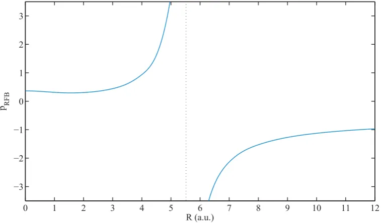
4.1 Variation of pRFB with the bond lengthR. . . 79

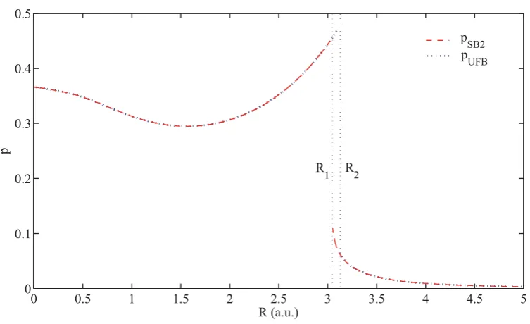
4.2 Variation of pUFB andpSB2 with the bond lengthR. . . 82

4.3 Single-ζ RHF, UHF, RFB , UFB and CI potential energy curves for H2. . . 84

4.4 Variation of the RFB and symmetry broken STO-1G electronic energies withR 85

4.5 Variation of the UFB/STO-1G energy function with mixing parametert . . 86

2.1 The free-complement ground state (X2Σ+_g) electronic energyE, and exponent ζ, for the hydrogen molecular ion H+₂ atR=2. . . 23

2.2 The free-complement singlet ground state (1S) electronic energy E, and

exponentζ, for the helium atom. . . 27

2.3 The first triplet excited state (3S) FC electronic energy (E orEb)a of the helium atom with the electronic configuration 1s2s. . . 31

2.4 The variational electronic energyE, exponentsζ andβ and linear correlation

coefficient pfor the singlet ground state of the helium atom. . . 35

4.1 Single-zeta electronic energiesE, exponentsζ, mixing parameterst, and

lin-ear coefficients pfor H2at bond lengthR. The boldface numbers correspond

to the lowest energy UFB solution. . . 75

4.2 Equilibrium bond length Re, harmonic vibrational frequencyωe and well

the interval[0,1]. . . 125

D.1 The optimized coefficientsc_μ and exponentsαμ for the normalized STO–8G

List of Abbreviations

and Nomenclatures

Acronyms / Abbreviations

AO Atomic Orbital

BO Born-Oppenheimer

CC Coupled Cluster

CCS Coupled Cluster Singles

CCSD Coupled Cluster Singles and Doubles

CHGF Confluent Hypergeometric Function

CI Configuration Interaction

CMO Correlated Molecular Orbital

CSF Configuration State Function

FB Frost-Braunstein

FCI Full-Configuration Interaction

GTO Gaussian-Type Orbital

HF Hartree-Fock

HP Hartree Product

ICI Iterative Configuration Interaction

ISE Inverse Schrödinger Equation

LSE Local Schrödinger Equation

LYP Lee–Yang–Parr

MO Molecular Orbital

PEC Potential Energy Curve

RFB Restricted Frost-Braunstein

RHF Restricted Hartree-Fock

SB Symmetry-Broken

SCF Self-Consistent Field

SE Schrödinger Equation

SSE Scaled Schrödinger Equation

STO Slater-Type Orbital

UFB Unrestricted Frost-Braunstein

CHAPTER

1

Electron Correlation and Explicitly Correlated

Wavefucntions

of the wavefunction, i.e., the slow convergence of the energy to the basis set limit, the origins of the ideas of introducing the interelectronic distance into the wavefunction were discussed. Atomic units have been used throughout this thesis.

1.1

Introduction to the Correlation Problem

As one of the most fundamental characteristics of the many-electron systems and based on

the probabilistic interpretation of the quantum mechanics, [1] the electron correlation can

find its roots in the correlation concept arising in probability theory [2, 3]. This issue is

of crucial importance in quantum chemistry possibly because most popular approximate

methods in this field are based on independent particle model or mean–field approach to

describe theN-electron systems. [1, 4] Therefore, because of relying on the independent

particle or mean–field models, one makes an error that is considered ascorrelation problem.

[1, 5, 6] There are two main sources responsible for the electron correlation: [1, 5]

i. Fermi Correlation: Electrons as countable but indistinguishable fermions should obey

Fermi statistics and satisfy the Pauli principle meaning that theN-electron wavefunction

should be antisymmetric with respect to the simultaneous exchange of the (spatial and

spin) coordinates of any pairs of electrons.

ii. Coulomb Correlation: Electrons as charged particles repel each other through

(pair-wise) Coulombic electrostatic forces.

In relation to the concept of electron correlation, one can refer to the Löwdin’s classical

definition of thecorrelation energywhich is the difference between the exact non-relativistic

energy and the restricted Hartree-Fock (RHF) energy: the lowest variational energy obtainable

with a single-determinant wavefunction. [7] Pople and Binkley extended the scope of this

definition to the unrestricted HF (UHF) wavefunctions. [8] However, these definitions

encourages the quantum chemistry community to abandon these traditional definitions in

favor of a modern definition of the correlation energy which intrinsically arises in the

second-quantization formulation in Fock-space using the cumulants [9–14] of the density matrices.

[1]

1.1.1

Electron Correlation in Statistical Sense

Let us assume two variables, say,x₁andx₂in a two-variable distribution with the (joint or

pair) probability distribution functionP12(x1,x2). The individual (or marginal) probability distribution functions for each variable can be obtained by integrating out the other variable,

i.e., [3]

P1(x1) =

P12(x1,x2)dx2 or P2(x2) =

P12(x1,x2)dx1 (1.1)

The two variables,x1andx2are independent from each other if [15, 16]

P12(x1,x2) =P1(x1)P2(x2) (1.2)

For distinguishable particles, the individual probability distribution functionsP1(x1)and

P₂(x₂)can be different from each other and hence, the pair probability distribution function

P₁₂(x₁,x₂)may be different for every particle pair. [5] Let Ψ(x₁,x₂,x₃,...,xN) be anN

-electron wavefunction in which,xicollectively shows the spatial,riand spin,ωicoordinates.

The electrons are indistinguishable particles and therefore, P1(x1) =P2(x2). Hence, the normalized one-electronρ(x)and pair densitiesρ2(x1,x2)can be defined as

ρ(x) =NP₁(x₁) (1.3)

where

P₁(x₁) =

dx₂···

dxN Ψ∗(x1,x2,x3,...,xN)Ψ(x1,x2,x3,...,xN) (1.5)

P12(x1,x2) =

dx3···

dxN Ψ∗(x1,x2,x3,...,xN)Ψ(x1,x2,x3,...,xN) (1.6)

Here,P₁(x₁)shows the probability of finding an electron atx₁, and the pair densityP₁₂(x₁,x₂) is the probability of finding an electron atx1and simultaneously, another electron atx2. [5]

When the electrons are (statistically) uncorrelated or independent, one can write

ρ2(x₁,x₂) = N−1

N ρ(x1)ρ(x2) (1.7)

In the non-relativistic regime, each electron can be described by a spin-orbitalχ(x)which is the product of a spatial functionψ(r)of the position vectorrand one of the two orthonormal spin functionsα(ω)(spin-up) orβ(ω)(spin-down),i.e.[17]

χ(x) = ⎧ ⎪ ⎪ ⎪ ⎪ ⎨ ⎪ ⎪ ⎪ ⎪ ⎩

ψ(r)α(ω)≡ψ(r) or

ψ(r)β(ω)≡ψ(r)

(1.8)

Also, an equivalent notation has been presented in Eq. 1.8 by which, each spin-orbital is

1.1.2

Hartree Product and Slater Determinants

The general form for the Hartree product (HP) can be written as [1, 5, 17]

ΨHP_(x

1,x2,x3,...,xN) = N

∏

i=1

χi(xi) (1.9)

where χ(x) are orthonormal spin-orbitals. The form of the HP wavefunction implicitly assigns each electron to a specific spin-orbital and thus, incorrectly assumes that the electrons

are distinguishable particles. Hence, for every pair of electronsiand j, there is a different set

of one- and two-particle probability distribution functions

Pi(xi) =χi∗(xi)χi(xi) (1.10a)

Pj(xj) =χ∗j(xj)χj(xj) (1.10b)

Pi j(xi,xj) =Pi(xi)Pj(xj) (1.10c)

Here, the contentious issue of the presence of the electron correlation in the electronic HP

wavefunction arises. Based on Eqs. 1.10a-1.10c, a large group of quantum chemists believe

that the HP wavefunction is statistically uncorrelated. [17] However, the second group of

scientists, for which, we directly quote Hättiget al.’s [5] comments as an example, show

that the HP wavefunction for an electronic system is statistically correlated. Considering

Eqs. 1.10a-1.10c, they say: "Since for every pair (of electrons), the two-particle probability

distribution function factorizes into a product of one-particle distribution functions, one may

be tempted to say that the electrons are statistically uncorrelated (Eq. 1.2). This is only true

if the electronic coordinates are treated as distinguishable. However, because electrons are

Eq. 1.7. For the HP wavefunction, the density and pair density functions take the form of

ρ(x₁) =

N

∑

i=1

Pi(x1) (1.11)

ρ2(x₁,x₂) =

N

∑

i,j=1

i=j

Pi j(x1,x2) (1.12)

which leads to

ρ2(x1,x2) =ρ(x1)ρ(x2)−

N

∑

i=1

Pi(x1)Pi(x2) (1.13) Regarding Eq. 1.13, Hättiget al.[5] then add: "Thus, the electron pair probability distribution

derived from a Hartree product wavefunction is statistically correlated." Note that in Eq.

1.12, one must exclude the i= j term from the summation. In order to provide further understanding of the nature of the correlation, existing in HP wavefunction, the authors of

Ref. [5] present another example in which, they consider HP wavefunction for a specific

state of bosonic particles. In this bosonic system, all particles can occupy the same orbitals.

It can be easily shown that in such a system, described by the HP wavefunction, the particles

are statistically uncorrelated. [5] Kutzelnigg also comments on this issue using the same

strategy. [1] He mentions: "With the just given definition of independent electrons (Eq. 1.7),

even a Hartree product does not generally describe independent electrons, since the density

and the pair density given by Eqs. 1.11 and 1.12, respectively, do not satisfy Eq. 1.7." [1] He

refers to the ground state of the two-electron atom described by the HP wavefunction and the

electron gas described by a HP of plane wave states as exceptions where the HP can describe

them as systems of independent particles. [1]

There are positive [1] and negative criticisms [1, 5] about the HPs. The criticisms are

i. The HP does not fulfill the Pauli principle and implies that the electrons are

dis-tinguishable particles. There is a different effective one-particle operator for each

spin-orbital.

ii. The HP is not invariant with respect to a unitary transformation among the occupied

spin-orbitals. [1]

iii. The HP wavefunction is an eigenfunction of the ˆSzoperator but not an eigenfunction

of the total spin operator ˆS2, generally.

As noted by Slater, [19], an improvement over the HP ansatz can be made by using

a linear combination of HPs [17] which satisfies the Pauli principle. Considering a set

of M (orthonormal) spatial orbitals {ψi|i=1,2,...,M}, one can construct a set of 2M

(orthonormal) spin-orbitals{χi|i=1,2,...,2M}. Using this set of spin-orbitals, a Slater

determinant, describing the simplest antisymmetric wavefunction [20] for a N-electron

system, can be constructed as [4, 17]

Ψ(x1,x2,...,xN) =

1 √

N!

χi(x1) χj(x1) ... χk(x1) χi(x2) χj(x2) ... χk(x2)

..

. ... ...

χi(xN) χj(xN) ... χk(xN)

(1.14)

= √1

N! A

N

∏

i=1

χi(xi) (1.15)

in which, theN-electron antisymmetrizer,A, is defined as [1, 5]

A=

∑

q=1

where depending on the parity of the permutation,Pq, the Levi-Civita symbolεtakes the

value of [3]

εq=

⎧ ⎪ ⎨ ⎪ ⎩

+1 even permutation

−1 odd permutation

(1.17)

Compared with the HP, the wavefunction approximated by the Slater determinant(s) satisfies

the Pauli principle and is invariant under the unitary transformation among the occupied

spin-orbitals, [1]. The Slater determinants are the eigenfunction of ˆSz operator, and also,

the eigenfunctions of the total spin operator ˆS2 for electronic states with closed-shell or

high-spin open-shell configurations. However, for low-spin open-shell configurations, one

can use configuration state functions (CSFs) that can be the eigenfunctions of both ˆSz and ˆS2

operators. Generally, CSFs are defined as the linear combination of the Slater determinants.

[21]

For a wavefunction approximated by a single Slater determinant, the one-electron and

pair densities can be expressed as

ρ(x) =NPi(x) = N

∑

i=1

χi(x)χi∗(x) (1.18)

ρ2(x1,x2) =ρ(x1)ρ(x2)− N

∑

i₌1

Pi(x1)Pi(x2)

=

∑

i,j=1 i=j

χi(x1)χj(x2)χi∗(x1)χ∗j(x2)−χi(x1)χj(x2)χj∗(x1)χi∗(x2) (1.19)

Note that the inclusion of the i= j term in Eq. 1.19 leaves the pair density unchanged because this contribution would be canceled between the first (direct) and second (exchange)

terms in the square brackets. Therefore, one can safely remove thei= jrestriction from the summation. However, exclusion of the self-pairing contribution in the HP case was necessary

because of the Pauli principle. [1] Considering a Slater determinant for a two-electron

wavefunction and Eq. 1.19, one can easily verify that there is a finite probability of finding

electrons of parallel spins,ρ2(r1,r1) =0 and one can speak of the existence of theFermi hole around each electron. [5, 17] Kutzelnigg criticizes statements such as "there is a negative

Fermi correlation for electrons with the same spin and no correlation for electrons with

opposite spin." [1] He shows that what is crucial is not the individual spins of the electrons

but the total spin to which, their spins are coupled.

1.1.3

Electron Correlation in Qualitative Sense

The conceptual explanation and pictorial intuition can be achieved for the electron correlation

using simple descriptors which are based on the pair density functions and arise in both

Fermi and Coulomb correlation contexts. These are [1, 5]

i. Radial (or in-out) correlation: If an electron spends most of its time close to a nucleus,

it is more probable for the other electron(s) to be found far out from the nucleus.

ii. Angular correlation: If one electron is on one side of the nucleus, the other electron is

more likely to be found on the opposite side.

iii. Left-right correlation: If an electron spends most of its time close to a nucleus, it is

more probable for the other electron to be found close to the other nucleus.

The radial and angular descriptors are convenient for describing the electron correlation

in atoms or for regions which are close to nuclei in molecules. The left-right correlation,

however, is useful for describing the electron correlation in the regions between atoms in

molecules. [5] To exemplify these concepts, one can consider the leading configuration in

the ground state of the H2molecule, which is 1σg2, the admixture of which with the 2σg2and

1π_u2configurations can account for the radial and angular correlation, respectively. [1] In chapter 4, we will see in the configuration interaction (CI) calculation on the ground

state energy of the H2molecule that mixing the 1σg2state with 1σu2state leads to a negative

to each other in space. This correlation is purely due to the Coulombic repulsion force

between the electrons. [5] From this CI picture, in which different CSFs can mix, the notion

ofstatic correlationemerges. On the other hand, one can speak ofdynamic correlationwhen

(compared to the mean-field picture) an electron can "feel" the instantaneous interaction with

another electron when they are in similar regions of space.

1.1.4

Electron Correlation in Quantitative Sense

Probability theory not only provides us a way to define the electron correlation from the

statistical point of view, but also a tool to "measure" it. Considering the two variablesxand

yof individual probability densitiesP1(x)andP2(y), respectively, and the joint probability densityP12(x,y), one can define the mean valuesx andy , the variancesσx2andσy2[3]

x =

_∞

−∞x P1(x)dx y = _∞

−∞y P2(y)dy (1.20a) σ2_{(x) =} ∞

−∞(x− x ) 2_P

1(x)dx σ2(y) =

_∞

−∞(y− y ) 2_P

2(y)dy (1.20b)

and covariance, cov(x,y), as [3]

cov(x,y) =

_∞

−∞ _∞

−∞(x− x )(y− y ) P12(x,y)dxdy (1.21)

It can be easily shown that the normalized covariance (or correlation coefficient,τ) is bounded

between -1 and 1. [3], In other words

τ= cov(x,y)

σ(x)σ(y); −1≤τ≤+1 (1.22)

measures of the electron correlation such as radial,τr, and angular,τa, correlation coefficients,

the vector variablesr1,r2 andr1·r2can be used inτ instead of the variablesx,yandxy, respectively. [15, 16] For example, for the ground state of the helium atom, the radial and

angular correlation coefficients are equal toτr=−0.112 andτa=−0.054, respectively. [1]

Other measures of correlation such as correlation entropy have also been proposed for the

quantitative description of the electron correlation. [22]

1.2

Explicit Correlation in Electronic Wavefunctions

After about nine decades from the discovery of the most fundamental equation in quantum

mechanics, the Schrödinger equation (SE), [23] the mystery of having the exact solution to

this equation, describing the correlated motion ofNinteracting particles, stands still except

for a small number of special cases. Considering the astonishing technological advancements

in the computational resources and albeit of numerical accuracy that one can achieve for

some small systems, even for the helium atom, [24] the exact analytic solution to SE is still

unknown. Consequently, adopting pragmatic approximations for solving the SE has been the

main focus of the quantum chemistry community so far. [4]

In construction of the trial wavefunction for variational calculations, one should retain as

many symmetries and properties of the exact wavefunction as possible. [4] For instance, the

wavefunction of fermions should be antisymmetric with respect to the permutation of any

pair of electrons. Some of the properties of the exact wavefunction have more crucial impacts

on the variational calculations with trial wavefunctions than the others, especially, when one

deals with highly accurate calculations. For example, based on the Kato’s analysis of the

properties of the exact wavefunction [25] near Coulomb singularities, [26] the eigenfunctions

of the N-electron SE are continuous and have bounded continuous first derivatives. [6]

The results of his work showed that the structure of the first derivative of the wavefunction

wavefunctions with the same types of singularities would be a more efficient approximation

to the exact solution. [6]

In 1927, for the first time, Slater proposed an approximate wavefunction including

the interelectronic distance which turned out to be a proper candidate for both core and

Rydberg limits of a two-electron atom. [27] About the same time, Hylleraas performed a

calculation on the ground state of the helium atom. [28] Hylleraas’ calculation showed that

compared with the slow convergence rate for the energy of the CI-type expansions, a rapid

convergence to the basis set limit can be achieved for the energy using explicitly correlated

wavefunctions. Adopting a three-term wavefunction, he managed to achieve a variational

energy ofE =−2.90243. [28] Following Hylleraas’ ideas, James and Coolidge designed a 13-term explicitly correlated wavefunction and used it for the ground state of the H2

molecule to obtainE=−1.173465 atR=1.4. They also generalized Hylleraas’ expansion for Li atom [29] which has been considered as the essence of the Hylleraas-configuration

interaction (Hy-CI) method [5] introduced by Preiskorn and Wo´znicki. [30] Since then, there

were numerous improvements in the field of explicitly correlated calculations in general

and on Hylleraas-type expansions, in particular. An interesting survey can be found in Refs.

[5, 6, 31]. Because of the complexity and difficulty of the many-electron integrals arising in

the explicitly correlated methods, the application of these methods has been mainly restricted

to highly accurate calculations on small systems.

Recent developments, however, have been mostly focused on invention of the practically

affordable methods for larger systems. The key paper on this route was published in 1985

by Kutzelnigg [32] who introduced the R12 method to show that the augmentation of the

reference determinant in the traditional CI expansion with the linearr₁₂ correlation factor,

satisfying the cusp condition, results in the rapid convergence of the energy to its basis

set limit value. [32] Kutzelnigg not only presented his result for the He atom and

systems. [5] Today, the R12 and (and its modified modern version F12) method [33, 34]

and its combinations with various standard correlated methods such as second-order

Møller-Plesset (MP2) perturbation and coupled cluster (CC) theories, [35] armed with mathematical

approximations and numerical methods to avoid direct calculation of many-electron integrals,

[5] have made it possible to have an acceptable balance between accuracy and computational

resources for larger systems of chemical interest.

1.3

Concluding Remarks

A brief introduction to the correlation problem in quantum chemistry is presented.

Consider-ing both qualitative and quantitative aspects of the electron correlation, different definitions

and concepts such as statistical interpretation of the electron correlation, radial, angular,

left-right, static and dynamic correlation were discussed. Regarding the slow rate of convergence

of the energy toward its basis set limit value in the CI-type expansions of the wavefunction,

the explicit insertion of the interelectronic distance in the wavefunction has been considered

as an efficient solution.

In the next chapter, we consider the free-complement (FC) method, which is based on the

theory of the structure of the exact wavefunctions presented by Nakatsuji. Through a careful

analysis, we will discuss the strengths and weaknesses of the FC method to be able to think

about the best way to construct a compact but efficient ansatz which is generalizable for large

CHAPTER

2

Structure of the Exact Wavefunction: Free

Complement Method

number. It can be shown that at a specific FC order, lower energies can be obtained using fewer complement functions. In the study of the first triplet excited state of the He atom, we have found that in addition to the determinants, permanents also appear in the FC expansion of the wavefunction. We have demonstrated that the presence of permanents in the FC expansion is important for the energy convergence. However, they have either been overlooked in Nakatsuji’s works or discarded because of their computational costs without any comments. These results led us to think about designing a new correlation factor F(r12)with which one can have an optimally compact and efficient wavefunction.

2.1

Introduction

In 2000, H. Nakatsuji began to report a series of studies under the topic of the structure of

the exact wavefunction. [36–40] He based the foundation of this research on the fact that the

exact"Hamiltonian is composed of only one- and two- particle operators and there are no

physical operators that involve more-than-three body interactions". [36] That is

H =F+G (2.1)

in which, the one-electron operatorF and two-electron operatorG have been defined in the

first-quantization as

F =

∑

i

−1 2∇

2

i −

∑

∑

ZA/riA (2.2)

G =

∑

i>j

or in the second-quantized form as

F =

∑

PQ

fPQa†_PaQ (2.4)

G = 1

2

∑

Pa

†

RaSaQ (2.5)

where in Eqs. 2.4 and 2.5, summations are over all spin-orbitals. [4, 41] Here, the creation

operatora†, and annihilation operatora, satisfy the anticommutation relations

a†_PaQ+aQa†P= [a†P,aQ]+ =δPQ

a†_Pa†_Q+a†_Qa_P† = [a†_P,a†_Q]+ =0

aPaQ+aQaP= [aP,aQ]+ =0

(2.6)

He then proposed two theorems to indicate the possibility of the description of the exact

wavefunction in terms of single and double excitations. [36] The first theorem is

Theorem 2.1.1 The wavefunctionΨthat satisfies both conditions

Ψ|(H −E)a†_PaQ|Ψ =0 (2.7a)

Ψ|(H −E)a†_Pa†_RaSaQ|Ψ =0 (2.7b)

is exact in a necessary and sufficient sense.

and the second theorem states that

Theorem 2.1.2 Assume thatΨhas the variables of the order of only singles and doubles

whereΦiis the given reference wavefunction. IfΨsatisfies the variational condition for the

coefficients cP_Qand cPR_QS, i.e.,

∂Ψ

∂cP_Q =a

†

PaQΨ (2.8b)

∂Ψ

∂cPR_QS =a

†

Pa†RaSaQΨ (2.8c)

thenΨis exact in the sufficient sense.

Note that theorem 2.1.2 is not a necessary condition because the space defined byΨin this theorem may be smaller than the real space of the exact wavefunction. Proof of both theorems

is presented by Nakatsuji. [36] Based on theorem 2.1.2, he considered the variational

exponential ansatz [36, 38, 39] and examined coupled-cluster singles (CCS), coupled-cluster

singles and doubles (CCSD) and full-configuration interaction (FCI) wavefunctions for these

conditions. [36] After this analysis, he proposed an ansatz based on the structure of the exact

wavefunction which satisfies both theorems 2.1.1 and 2.1.2. This is the starting point for his

free complement (FC) method’s proposal.

In his second paper in this series, Nakatsuji generalized the second theorem by dividing

the Hamiltonian intoND parts to obtain a set ofND equations which are equivalent to the

Schrödinger (SE) equation. [37] In this way, the FC method could be generalized to calculate

the exact wavefunction with ND variables where 1≤ND ≤m2+

m(m−1) 2

2

in which, m

is the number of active orbitals. [37] This method has been applied to molecular systems

using finite basis-sets. [40] Armed with inverse Schrödinger equation (ISE) [42] and scaled

Schrödinger equation (SSE) [43] which are equivalent to the SE and are proposed to remove

the nuclear and electronic singularity problems, the FC method has been further generalized

to its final form. This method is now considered as an analytic way of generating arbitrarily

accurate wavefunctions and energies the scope of which is again restricted to small systems

When the analytic form of the overlap and Hamiltonan matrix elements are not available,

Nakatsuji proposes the use of local SE (LSE) with the standard Monte Carlo sampling.

[44–46] In the present thesis, in order to be able to propose a compact form for an accurate

wavefunction for molecular systems, the analytic solutions to the explicitly correlated

prob-lems will be the main focus. Consequently, integral-free methods such as FC-LSE will not

be considered further.

2.2

Free-Complement Method and Scaled-Schrödinger

Equa-tion

We now embark on a more detailed analysis of the FC method within the framework of the

SSE. [24] The original form of SE

HΨ=EΨ (2.9)

where the general Hamiltonian defined in Eq. 2.1, has nuclear (Eq. 2.2) and electronic

(Eq. 2.3) singularities. Since the right-hand side of Eq. 2.9 has no singularities, these sharp

changes must be canceled out in the left hand side of this equation. In the case of the exact

wavefunction, satisfying the Kato’s cusp conditions, [26] no such singularities exist in the

SE. However, in case of an approximate wavefunction, this precise cancelation does not

happen and some of the matrix elements (e.g., those involving−1/rmfactor wherem≥3 or matrix elements in different ansätze) may diverge. [43] In the ISE scheme, one usesH −1 instead ofH and therefore, no such difficulties regarding to the singularities occur. [42]

One of the issues which arises in the ISE approach is that one needs to know how to write

the inverse Hamiltonian in closed form. [42] The SSE is free from such problems [43] and

can be written as

in which,gstands for the scaling factor which is a function of electron coordinates. [43]

This multiplicative operator,g, does not generally commute with Hamiltonian and is always

non-zero except at singular pointr₀where it can be zero. Thegfactor also satisfies

lim

r→r0

gV =0 (2.11)

whereV is the potential operator in the Hamiltonian. This condition is necessary because

gshould not eliminate information at singularity. There are various possible forms forg

function, [47] however, Nakatsuji favors the following form [24]

g=

∑

i

∑

riA+

∑

ri j (2.12)

The construction of the FC wavefunction in the SSE framework begins with the simplest ICI

(SICI) formula

Ψn+1= [1+Cng(H −En)]Ψn (2.13)

whereCnis the variational parameter at each ordern. The FC wavefunction is guaranteed

to converge to the exact solution of the SSE without encountering the singularity problem.

[43, 47] Applying thegandgH operators forntimes onΨ0in Eq. 2.13, the right-hand side of this equation becomes a sum of analyticalcomplement functionsφi

Ψn= Mn

∑

i=1

c(_in)φ_i(n) (2.14)

Here, the coefficients {c(_in)} are determined variationally [47] and Mn is the number of

complement functions. This is important to note that when one usesgandgH operators in

Eq. 2.13, some diverging functions are also generated in Eq. 2.14. Nakatsuji points out that

they should be discarded because the wavefunction must be integrable and finite. [24, 47]

the basis (complement) functions. [24] The functional form of the complement functions is

determined by the form of the initial wavefunctionΨ0. [24]

2.2.1

Free-Complement Electronic Energies

In the present section, we apply the FC method to calculate the energy of the H+₂ molecular

ion [48, 49], and He atom in both singlet ground [47] and triplet excited states. [50] We also

use spatial representation for constructing our initial wavefunctions because of its simplicity

and convenience in the absence of external fields. [18]

2.2.1.1 Hydrogen Molecular Ion: The Ground State

The H+₂ molecular ion is a special case of a molecular system for which, the exact solution

to the non-relativistic SE is known. [48, 49, 51] Because of the Born-Oppenheimer (BO)

approximation, this three-body problem can be reduced to one-body two-center problem in

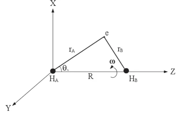
(confocal spheroidal or) elliptic coordinate system shown in Fig. 2.1. [52]

λ =rA+rB

R , μ =

r_A−rB

R , ω (2.15)

whereλ,μ andω are defined on the ranges of[1,∞),[−1,1]and[0,2π], respectively and the volume element isR3(λ2−μ2)/8. [52] Also,rAstands for the distance of the electron from centerA,rBis the distance of the electron from centerBandRis the distance between

two centersAandB(Fig. 2.1). In this coordinate system, the Hamiltonian operator can be

written as

H =− 2

R2(λ2−μ2)

∂ ∂λ

λ2₋₁ ∂ ∂λ +

∂ ∂ μ

1−μ2 ∂ ∂ μ +

λ2_−μ2 (λ2−₁)(₁−μ2)

∂2 ∂ω2

− 4λ

R(λ2−μ2)

Fig. 2.1 The hydrogen molecular ion H+₂ aligned on the Z axis in the elliptic coordinate system.

where the first line of Eq. 2.16 comes from the kinetic part and the second line results from

the nuclear-attraction term. [49] We need to choose an appropriate gfactor to eliminate

the singularity issue arising from the nuclear attraction term in the Hamiltonian. Therefore,

based on Eq. 2.12, thegfactor takes the form of [49]

g=− 1 VNe =

Rλ2−μ2

4λ (2.17)

The sign of theVNe is inverted to makegpositive everywhere except at singularity. Using

spatial notation, [18] the initial wavefunctionΨ0forX2Σ+g (or 1σg) gerade ground state of

H+₂ can be constructed as

Ψ0=exp[−ζ(rA+rB)] =exp(−ζλ) (2.18)

wavefunction

Ψ=

∑

i=1

ciλmiμniexp(−ζλ) (2.19)

in which,mican be a positive or negative integer andnican be zero or positive even integer

for the gerade ground state (X2Σ+_g) of H+₂. [49] Considering the general form of the FC wavefunction, the Hamiltonian and overlap matrix elements over complement functions{φi}

become

φi|H|φj =

R3 8 _2π 0 ₁ −1 _∞ 1

λmiμni_e−ζλ

H λmjμnj_e−ζλλ2−μ2 dλ _dμ dω _(2.20a)

φi|φj =

R3 8 2_π 0 1 −1 _∞ 1

λmiμni_e−ζλ

λmjμnj_e−ζλλ2−μ2 dλ dμ dω _(2.20b)

The explicit forms for the integrals can be obtained using a symbolic mathematical program

package such asMathematica[53] or can be found in Nakatsuji’s paper. [48] Solving the

generalized eigenvalue equation and diagonalizing the Hamiltonian matrix with respect to

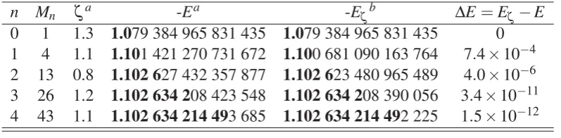
the overlap matrix gives the energies that are shown in Table 2.1.

Table 2.1 The free-complement ground state (X2Σ+_g) electronic energyE, and exponentζ, for the hydrogen molecular ion H+₂ atR=2.

n Mn ζa -Ea -E_ζb ΔE=E_ζ−E

0 1 1.3 1.079 384 965 831 435 1.079 384 965 831 435 0 1 4 1.1 1.101 421 270 731 672 1.100 681 090 163 764 7.4×10−4 2 13 0.8 1.102 627 432 357 877 1.102 623 480 965 489 4.0×10−6 3 26 1.2 1.102 634 208 423 548 1.102 634 208 390 056 3.4×10−11 4 43 1.1 1.102 634 214 493 685 1.102 634 214 492 225 1.5×10−12

a_{Refs. [48, 49]} b_E

ζ is the FC energy calculated using a fixed value ofζ =1.3 for the exponent.

The first row of this table shows a simple variational calculation usingΨ0 in minimal basis model. In order to find the optimized energy and the exponent for the minimal basis,

one can normalizeΨ0

1=Ψ0|Ψ0 = R 3 8C

2 2π 0

₁

−1

_∞

1 exp(−2ζλ)

to get

Ψ0=

24ζ3e2ζ

πR3_(4ζ2_+6ζ+3)

1/2

exp(−ζλ) (2.22)

Assumingζ >0, the Hamiltonian matrix element in Eq. 2.20b becomes

E= Ψ0|H |Ψ0

Ψ0|Ψ0 = R3

8

24ζ3e2ζ

πR3(₄ζ2+₆ζ+₃)

2π

0

₁

−1

_∞

1

exp(−ζλ)H exp(−ζλ)λ2−μ2 dλ dμ dω

= 6₍ζ(2ζ+1)(ζ−2R)

4ζ2_+6ζ+3)R2

(2.23)

The potential energy curve (PEC) is produced after adding the 1/Rnuclear repulsion term

to the optimized electronic energy at each specific bond length. At Re ≈2.00, [54] the

optimized exponent and the electronic energy for the minimal basis model areζ =1.3337··· andE =−1.079 754 641···, respectively. Note that the difference in the calculated energy presented here compared with that demonstrated in the first row of the Table 2.1 comes

from the difference between the number of digits considered for ζ in the corresponding

calculations.

The FC energies in the fourth column of Table 2.1 were reproduced using the optimal

values forζ reported in Refs. [48, 49] and agree perfectly with the energies presented in

these references. The number of accurate digits, shown in boldface, increases as the structure

of the FC wavefucntion converges to the exact solution of the SE with increasing the FC

order,n.

The FC energies calculated using the fixed exponentζ =1.3 and energy differences are collected in fifth and sixth columns of Table 2.1, respectively. These values demonstrate

that fixing the exponent to its initially optimized value has small effect on the calculated

FC energy at higher orders. In fact, the number of accurate digits remains unchanged in

and keep it fixed during the FC calculations. The initial guess exponents can be obtained in

a minimal–basis variational calculation or can be estimated from Slater’s rules [55]. This

eliminates the cost of non-linear optimization which is both time-consuming and difficult at

higher orders.

2.2.1.2 Helium Atom: The Ground State

Since the ground state of the helium atom has zero spatial angular momentum orSsymmetry,

we adopt Hylleraas{s,t,u}interparticle coordinates defined as

s=r1+r2

t=r₁−r₂ u=|r1−r2|=r12

(2.24)

to solve the SSE (or equivalently SE) using FC method. In this coordinate system, [56] the

nucleus is considered to be fixed at the origin. Hence, the Hamiltonian can be written as

H =−

∂2 ∂s2+

∂2 ∂t2+

∂2 ∂u2

−2s(u 2_−t2₎

u(s2_−t2₎ ∂2 ∂s∂u−2

t(s2−u2) u(s2_−t2₎

∂2 ∂u∂t −

4s s2_−t2

∂ ∂s

−2

u

∂ ∂u+

4t s2−_t2

∂ ∂t−

4sZ s2−_t2+

1

u

(2.25)

where the last two terms in this equation belong to the Coulomb potential

V =VNe+Vee=− 4

sZ s2_−t2+

1

u (2.26)

in which,Zis the nuclear charge. The remaining terms in Eq. 2.25 come from the kinetic

part. According to Eq. 2.12, we choosegsuch that

g=

8s s2_−t2

where for the He atom,Z=2. The sign of theVNeis inverted to makegpositive everywhere

except at singularity. Neglecting the spin part, our initial guess in spatial form would be the

product of two atomic orbitals (AOs) for two electrons

Ψ0=exp[−ζ(r1+r2)] =exp(−ζs) (2.28)

Applying theg andgH operators onΨ0 in Eq. 2.13 and removing the duplications and singular terms, one finds that Eq. 2.14 becomes

Ψ1=

c1s0t0u0+c2s−1t2u0+c3s1t0u0+c4s0t0u1 exp(−ζs) (2.29)

continuing the FC process to higher orders,i.e., applyinggandgH operators in a consecutive

way, one discovers that the generated FC wavefunctions have the general form of

Ψ=

∑

i=1

cislitmiuniexp(−ζs) (2.30)

whereci is the variational parameter. For singlet state, li runs over all integers while, mi

is a non-negative and even integer andni runs over all non-negative integers. [47] By the

present choice of thegfactor (Eqs. 2.12 and 2.27), the negative powers of the variables

are also generated in the{s,t,u}expansion of the FC wavefunction (Eq. 2.30). In 1957, Kinoshita [57] reported the importance of the inclusion of the negative powers ofsin the

wavefunction expansion for which, the resulting energy was remarkably improved compared

with the ansätze that were bereft of these terms.

Instead of the tedious way of applying the FC operators, Nakatsuji proposed a

combina-tion of equalities and inequalities- the condicombina-tions imposed on{li,mi,ni}for generating the

ramifications for the first triplet excited state of the helium atom. This issue will be discussed

in the next subsection.

The general Hamiltonian and overlap matrix elements over the complement functions

{φi}become [56]

φi|H|φj =2π2

_∞

0

s

0

s

t

sli_tmi_uni_e−ζs

H slj_tmj_unj_e−ζs_s2−_t2 _{u du dt ds (2.31a)}

φi|φj =2π2

_∞

0

s

0

s

t

sli_tmi_uni_e−ζs

slj_tmj_unj_e−ζs_s2−_t2 _{u du dt ds (2.31b)}

The explicit forms for the integrals can be achieved usingMathematica[53] or can be looked

up in Nakatsuji’s paper. [47] Diagonalizing the Hamiltonian matrix with respect to the

overlap matrix gives the energies that are shown in Table 2.2.

Table 2.2 The free-complement singlet ground state (1S) electronic energyE, and exponent ζ, for the helium atom.

n Mn ζ -E -Eζa ΔE=Eζ−E

0 1 1.688 2.847 656 250 2.847 656 250 0 1 4 1.690 2.901 338 005 2.901 337 708 3.0×10−7 2 16 1.736 2.903642 984 2.903638 631 4.4×10−6 3 37 1.779 2.903 720 264 2.903 719 381 8.8×10−7 4 71 1.837 2.903 724019 2.903 723761 2.6×10−7

a_E

ζ is a FC energy calculated using a fixed value ofζ=27/16 for the exponent.

Here, the boldface digits show the exact and accurate digits (after rounding up to a

specific decimal place) in the energy. NormalizingΨ0=Ce−ζs (Eq. 2.28) using Eq. 2.31b and solving the equation forC,

1=Ψ0|Ψ0 =2π2C2

_∞

0

_s

0

_s

t e

one can find thatC=ζ3/π. Assumingζ >0, the minimization of the energy with respect to ζ using Rayleigh-Ritz technique [3]

E= Ψ0|H|Ψ0

Ψ0|Ψ0 =2π2

_∞

0

_s

0

_s

t

s2−t2 u

ζ3 π e−ζs

H

ζ3 π e−ζs

du dt ds

=ζ2₋27 8 ζ

(2.33)

gives the well-known [58] values ofE=−(27/16)2andζ =27/16 for the helium atom. The first-order FC energy (second row in Table 2.2) can be obtained through

diagonaliza-tion of the 4×4 Hamiltonian matrix with respect to the overlap matrix in the generalized eigenvalue equation. The process is almost the same for higher orders as well. The fifth

col-umn of the Table 2.2 shows the FC energiesE_ζ calculated using the fixed value ofζ =27/16 for the exponent. As is shown by the last column of the Table 2.2, the non-linear optimization

of the exponent can contribute to the energy at sixth decimal place or higher. Thus, depending

on the accuracy that we are seeking and/or the number of non-linear parameters that may

be optimized, fixing the exponent(s) to a reasonable value makes the FC calculations faster

because the bottleneck of the FC calculations becomes the diagonalization of the Hamiltonian

matrix.

In Table 2.2, one can see that as we increase the order, the energy and the structure of

the FC wavefunction become closer to being exact as it is guaranteed by the theorems 2.1.1

and 2.1.2. Comparing the data in Tables 2.2 and 2.1 and considering the boldface digits, one

can see that the convergence rate for the H+₂ is faster than that of the helium atom. This is

possibly because of the presence of the electronic cusp in the He atom. Although initially, the

rate of convergence in terms of acquiring more accurate digits is quite rapid with increasing

add only one more exact digits (at the tenth decimal place) to the energy. As discussed by

Bartlett, [59] Gronwall [60] and Fock, [61, 62] fulfilling the three-body collision conditions

may become an important factor for obtaining highly-accurate results. Nakatsuji adopted

various ansätze inserting the interelectronic distance in the logarithmic form into the initial

wavefunction to achieve an accuracy of over 40 digits in the energy of the ground state of the

helium atom usingMn=22709 complement functions generated at the order ofn=27. [47]

It is important to note that at a specific FC order, lower energies can be obtained using

fewer complement functions. For instance, the energy of the first-order FC wavefunction

(Table 2.2) with four terms (E =−2.9013) can be compared with that of the optimized three-terms Hylleraas wavefunction (E =−2.9024)) [63]. We have verified this fact for second-order where lower energy was obtained with the number of terms fewer than 16.

Although the structure of the FC wavefunction converges to that of the exact wavefunction

at then→∞limit, one can be more efficient by generating fewer but energetically more important functions.

2.2.1.3 Helium Atom: The Triplet Excited State

The FC method is equally applicable to both ground and excited states in the sense that

when one tries to find the variational energies by diagonalizing aMn×MnHamiltonian, the

approximate ground and excited state energies (of the same symmetry) are obtained within

a same eigenvalue problem. [50] Therefore, similar to the helium in the ground state, we

can use the FC method to calculate the first triplet excited state energy with the electronic

configuration 1s2s. The Hamiltonian operatorH and thegfactor remain the same as those

introduced in Eqs. 2.25 and 2.27 for {s,t,u} coordinate system. As noted by Nakatsuji, [50], in order to calculate the energy of the 1sNsstate of the helium atom, at least aboutN

because of the antisymmetric spatial part of the triplet state [18] and also the fact that the 2s

orbital is more diffuse than the 1sorbital. Dropping the spin part, the initial wavefunction

can be expressed as

Ψ0=

e−αr1 _e−βr1

e−αr2 _e−βr2

=

e−α(s+t)/2 e−β(s+t)/2 e−α(s−t)/2 e−β(s−t)/2

(2.34)

The normalization factor forΨ0can be found through

1=Ψ0|Ψ0 =2π2C2

_∞ 0 _s 0 _s t

e−α(s+t)/2 e−β(s+t)/2 e−α(s−t)/2 e−β(s−t)/2

2

s2−t2 u du dt ds (2.35)

to give the normalizedΨ0as

Ψ0=

2π2

1

α3_β3− 64

(α+β)6

₋1/2

e−α(s+t)/2 e−β(s+t)/2 e−α(s−t)/2 _e−β(s−t)/2

(2.36)

Assumingα >0 andβ >0, the Rayleigh-Ritz expression for obtaining the variational energy

is

E =Ψ0|H |Ψ0

Ψ0|Ψ0 =2π2

2π2

1 α3β3−

64

(α+β)6

−1 × ∞ 0 _s 0 _s t

s2−t2 u

e−α(s+t)/2 e−β(s+t)/2 e−α(s−t)/2 e−β(s−t)/2

H

e−α(s+t)/2 e−β(s+t)/2 e−α(s−t)/2 e−β(s−t)/2

du dt ds

=α2

2 + β2

2 −2α−2β+

αβα3_+8α2_β+32α2_β2_+8αβ2_+β3 α4+₈α3β+₃₀α2β2+₈αβ3+β4

(2.37)

Minimizing the energy expression with respect to the exponentsα andβ can result in the

β =0.3210··· to arbitrary accuracy. The difference between the variational energy value presented here and the energy value reported in the first row and third column of the Table

2.3 comes from the different number of digits considered for the exponents.

Table 2.3 The first triplet excited state (3S) FC electronic energy (E orEb)aof the helium atom with the electronic configuration 1s2s.

n Mn -E Mn b -Eb ΔE=Eb−E

0 1 2.160 644 009 1 2.160 644 009 0

1 4 2.161 240 437 5 2.163 221 387 -0.001 980 950

2 16 2.168 856 982 21 2.173 532 754 -0.004 675 772

6c 5724 2.175 229 378 236 791 305 738 966 – – –

a_{The exponents of the 1sand 2sorbitals were optimized for the minimal basis and kept fixed toα=1.97}

andβ =0.32 during the FC calculations.

b_{The primed values were calculated using FC wavefunctions that included the permanents in addition to}

the usual complement functions generated during the FC process.

c_{Ref. [48] The initial wavefunctionΨ}

0included 6 exponential functions in this calculation.

Beginning the FC procedure by applying the gand gH operators onΨ0 in Eq. 2.34 and removing the duplications and singular terms, one finds that the general form of the

FC wavefunction becomes different from our expectations. That is, in addition to having

a usual sum over antisymmetric determinants of Slater orbitals inΨ0, the symmetric anti-determinants or "permanents" also appear in the FC expansion.

Before presenting a simple definition for the permanents, we shall consider the Laplacian

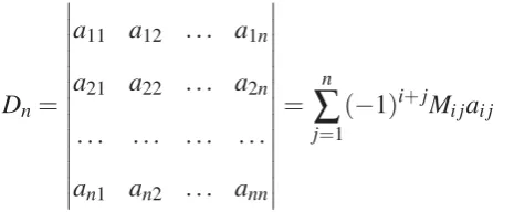
development of a generaln×ndeterminantDnin terms of minorsMi j [3]

Dn=

a11 a12 ... a1n

a21 a22 ... a2n

... ... ... ...

an1 an2 ... ann

=

∑

j=1

(−1)i+jMi jai j (2.38)

where the minorMi j, corresponding to the elementai j, is defined as a determinant of order

The factor(−1)i+jMi j is calledcofactorof the element ai j. In this way, determinants (as

well as permanents) are polynomials in entries of the matrix. [3]

Permanents can be considered as an analog of a determinant in which, all signs in the

expansion by minors in Eq. 2.38 are taken as positive. For example, the permanent of a 2×2 matrixAwill be

perm(A) =

a11 a12

a₂₁ a₂₂

+ +

=a11a22+a12a21 (2.39)

where the "perm()" as well as the vertical bars with plus signs, | |

+ +, indicate permanents.

[64, 65] After this short digression, we get back to the FC expansion (Eq. 2.14) which now

includes both determinants and permanents

Ψ=M

n

∑

i=1

cislitmiuni

e−α(s+t)/2 e−β(s+t)/2 e−α(s−t)/2 e−β(s−t)/2

+

c_islitmiuni

e−α(s+t)/2 e−β(s+t)/2 e−α(s−t)/2 e−β(s−t)/2

+ + (2.40)

wherem_iandmirun over odd and even positive integers, respectively. Also,liandl_ivary

over all integers andniandn_irun over all non-negative integers. Note that the multiplications

of either the odd polynomial part with permanents or even polynomial part with determinants

generates correct symmetry for the spatial part of the triplet state. The new FC wavefunction

Ψshould be compared with that which results from applying Nakatsuji’s rules and conditions (Table 1 in Ref. [50]) imposed on{li,mi,ni}using different numbers of exponential functions

inΨ0. Based on his FC method, we have used the minimum number of exponential functions (N =2) in the initial wavefunction to calculate the energy of the 1s2s triplet state of the helium atom. The results of these calculations are gathered in Table 2.3. This table clearly

shows that including the permanents in the FC calculations although is not favorable from

FC wavefunction seems necessary for obtaining a faster convergence to the desired accuracy

in the calculated energy values.

2.2.2

Examples of Compact Explicitly Correlated Wavefucntions: A

Case Study

Seeking the optimal forms for theN-term Hylleraas [66–68, 63] and the Kinoshita

wave-functions, [67, 69, 70], Koga performed several investigations with different optimization

techniques on these two wavefunctions for the helium atom and helium-like ions. He showed

that, for positive integer values of{li,mi,ni}in Eq. 2.30, the optimal form of aN-term

Hyller-aas wavefunction depends on the nuclear chargeZ. [68, 63] The reason of this observation

has been related to the different significance in the radial and angular correlation effects. In

this way, based on Eq. 2.24, it may be inferred that the terms including the variablessand

tcontribute mainly to the radial correlation energy whereas terms involving the variableu

mainly contribute to the angular correlation energy. [68, 63]

An important lesson than can be learnt from Koga’s studies on the N-term Hylleraas

wavefunctions is that the perturbational approaches are inappropriate for finding the optimal

form of the Hylleraas expansion shown in Eq. 2.30. [68, 63] This is because of the fact that

the terms that appear in the optimalN-term Hylleraas expansion does not necessarily appear

in the optimalN-term expansion of the same form whereN>N. [68, 63] Konget al.[6] performed an experiment (Tables 2 and 3 in Ref. [6]) on the calculation of the energy of the

helium atom using the 3-term Hylleraas expansion of the form