Mapping from parametric characteristics to generalized frequency response functions of nonlinear systems

This is a repository copy of Mapping from parametric characteristics to generalized

frequency response functions of nonlinear systems.

White Rose Research Online URL for this paper: http://eprints.whiterose.ac.uk/74629/

Monograph:

Jing, X.J., Lang, Z.Q. and Billings, S.A. (2008) Mapping from parametric characteristics to generalized frequency response functions of nonlinear systems. Research Report. ACSE Research Report no. 975 . Automatic Control and Systems Engineering, University of Sheffield

Reuse

Unless indicated otherwise, fulltext items are protected by copyright with all rights reserved. The copyright exception in section 29 of the Copyright, Designs and Patents Act 1988 allows the making of a single copy solely for the purpose of non-commercial research or private study within the limits of fair dealing. The publisher or other rights-holder may allow further reproduction and re-use of this version - refer to the White Rose Research Online record for this item. Where records identify the publisher as the copyright holder, users can verify any specific terms of use on the publisher’s website.

Takedown

If you consider content in White Rose Research Online to be in breach of UK law, please notify us by

Mapping from Parametric Characteristics to

Generalized Frequency Response Functions

of Nonlinear Systems

X. J. Jing, Z. Q. Lang, and S. A. Billings

Department of Automatic Control and Systems Engineering The University of Sheffield

Mappin Street, Sheffield S1 3JD, UK

Mapping from Parametric Characteristics to

Generalized Frequency Response Functions

of Nonlinear Systems

Xing Jian Jing*, Zi Qiang Lang, and Stephen A. Billings

Department of Automatic Control and Systems Engineering, University of Sheffield Mappin Street, Sheffield, S1 3JD, U.K.

[email protected]

Abstract: Based on the parametric characteristic of the nth-order GFRF (Generalised Frequency Response Function) for nonlinear systems described by an NDE (nonlinear differential equation) model, a mapping function from the parametric characteristics to the GFRFs is established, by which the nth-order GFRF can directly be written into a more straightforward and meaningful form in terms of the first order GFRF, i.e., an n -degree polynomial function of the first order GFRF. The new expression has no recursive relationship between different order GFRFs, and demonstrates some new properties of the GFRFs which can explicitly unveil the linear and nonlinear factors included in the GFRFs, and reveal clearly the relationship between the nth-order GFRF and its parametric characteristic, and also the relationship between the nth-order GFRF and the first order GFRF. The new results provide a novel and useful insight into the frequency domain analysis and design of nonlinear systems based on the GFRFs. Several examples are given to illustrate the theoretical results.

Keywords: Generalised Frequency Response Function (GFRF), Nonlinear systems, Parametric characteristics, Nonlinear differential equation (NDE), Volterra series

1 Introduction

The frequency domain analysis of nonlinear systems has been studied for many years

(Taylor 1999, Solomou 2002, Pavlov 2007). Nonlinear systems can also be studied in the

response for a practical nonlinear system have been developed based on this concept (Bendat 1990, Billings and Lang 1996, Chua and Ng 1979, Jing et al 2007).

To compute the GFRFs of nonlinear systems, Bedrosian and Rice (1971) introduced the “harmonic probing” method, by which the higher order GFRFs of the harmonic expansion of the nonlinear system under study can be derived. By applying the probing method (Rugh 1981), algorithms to compute the GFRFs for nonlinear Volterra systems described by NDE model and NARX (Nonlinear Auto-Regressive model with eXogenous input) model were derived, which enable the nth-order GFRF to be recursively obtained in terms of the coefficients of the governing NARX or NDE model (Peyton-Jones and Billings 1989, Billings and Peyton-Jones 1990, Chen and Billings 1989). Based on the GFRFs, frequency response characteristics of nonlinear systems can therefore be investigated (Peyton Jones and Billings 1990, Yue et al 2005). These results are important extensions of the well known frequency domain methods for linear systems such as transfer function or Bode diagram, and provide a method to the analysis of nonlinear systems in the frequency domain. Although these progresses have been made and the GFRFs of nonlinear systems described by NARX model and NDE model can be determined effectively, it can be seen that the GFRF is in fact a multivariate complex valued function series in terms of model parameters defined in high dimensional frequency space, and consequently the existing recursive algorithms for the computation of the GFRFs can not explicitly and simply reveal the analytical relationship between system time domain model parameters and system frequency response functions in a clear and straightforward manner such that many problems remain unsolved regarding the characteristics of the GFRFs and the system output frequency response, including how the frequency response functions are influenced by the parameters of the underlying system, and the connection to complex non-linear behaviours. These inhibit the practical application and understanding of the existing theoretical results to a certain extent. In order to solve these problems, the parametric characteristics of the GFRFs were studied in Jing et al (2006), which effectively build up a mapping from the GFRF to its parametric characteristic and thus provides an explicit expression for the analytical relationship between the GFRFs and system time-domain model parameters. The significance of the parametric characteristic analysis of the nth-order GFRF is that it can clearly reveal what model parameters contribute to and how these parameters affect system frequency response functions including the GFRFs and output frequency response function. This provides an effective approach to the analysis of the frequency domain characteristics of nonlinear systems in terms of system time domain model parameters.

parametric characteristics of the GFRFs to the GFRFs is studied. By using this new mapping function, the nth-order GFRF can directly be recovered from its parametric characteristic as an n-degree polynomial function of the first order GFRF, keeping the explicit analytical relationship between the GFRF and system time-domain model parameters. Compared with the existing recursive algorithm for the computation of the GFRFs, the new mapping function enables the nth-order GFRF to be determined in a much more straightforward and meaningful structure. Note from the previous results that the higher order GFRFs are recursively dependent on the lower order GFRFs. This crossing relationship sometimes complicates the qualitative analysis and understanding of system frequency characteristics by using the nth-order GFRF. The new results can effectively overcome this problem, and unveil the system’s linear and nonlinear factors included in the nth-order GFRF more clearly. This provides a novel and useful insight into the frequency domain analysis and design of nonlinear systems based on the GFRFs, and can be regarded an important extension of the parametric characteristic theory established previously. Several examples are given to illustrate these results.

Nomenclature

) , , ( ₁

,q p q p k k

c L ₊ A model parameter in the NDE model, ki is the order of the derivative,

p represents the order of the involved output nonlinearity, q is the order of the involved input nonlinearity, and p+q is the nonlinear degree of the parameter.

) , ,

( 1 n

n j j

H ω L ω The nth-order GFRF )] , , ( , ), 1 , , 0 ( ), 0 , , 0 (

[ _{, , ,}

, L L L _1L4243

m q p q p q

p q

p q

p c c c K K

C

= +

= A parameter vector consisting of all the nonlinear parameters of the form c_p,q(k₁,L,k_p+q)

CE(.) The coefficient extraction operator ))

, , (

(H_n j ₁ j _n

CE ω L ω The parametric characteristics of the nth-order GFRF )

, ,

( _{1 n}

n j j

f ω L ω The correlative function of CE(H_n(jω₁,L,jω_n))

⊗ The reduced Kronecker product defined in the CE operator

⊕ The reduced vectorized summation defined in the CE operator )

( )

( )

( _{, ,}

,0 1 1

0q ⋅ p q ⋅ pkqk ⋅

p c c

c L A monomial consisting of nonlinear parameters

p x x xs s

s_{1 2}L A p-partition of a monomial cp0,q0(⋅)cp1,q1(⋅)Lcpk,qk(⋅)

i x

s A monomial of xi parameters of {cp0,q0(⋅),L,cpk,qk(⋅)}of the involved

monomial, 0≤xi ≤k, and s0=1

) ( ) (

:S_C n S_f n

n →

ϕ A new mapping function from the parametric characteristics to the correlative functions, S_C(n) is the set of all the monomials in the parametric characteristics and S_f(n)is the set of all the involved correlative functions in the nth order GFRF.

)) ( (s s

n _x The order of the GFRF where the monomial s_x(s) is generated )

, ,

( _{1 n}

n ω ω

λ L The maximum eigenvalue of the frequency characteristic matrix Θn

2 The nth-order GFRF for nonlinear systems and its parametric

characteristic

A large amount of nonlinear systems can be described by the following nonlinear differential equation (NDE) model

0 ) ( )

( )

, , (

1 0 , 0 1 1

1 ,

1

=

∑∑ ∑

∏

∏

= = =

+ + = =

+

+

M

m m

p K

k k

q p

p i

k k p

i k k q p q

p q p

i i i

i

dt t u d dt

t y d k

k

c L (1)

where () ()

0

t x dt

t x d

k k k

=

=

, p+q=m,

∑

∑

∑

= =

= +

+

⋅ ⋅

=

⋅ K

k K

k K

k

k, pq 0 0 pq 0

) ( ) ( ) (

1 1

L , M is the maximum degree of nonlinearity in terms of y(t) and u(t), and K is the maximum order of the derivative. In this model, the parameters such as c0,1(.) and c1,0(.) are linear parameters corresponding to the linear terms in the model, i.e., _k

k

dt t y d ()

and _k

k

dt t u d ()

for k=0,1,…,L, and c_p,q(⋅) for p+q>1 are referred to as the nonlinear parameters corresponding to nonlinear terms in the model of the form

∏

∏

+ + = =

q p

p i

k k p

i k k

i i i

i

dt t u d dt

t y d

1 1

) ( )

(

, e.g., _y(t)p_u(t)q_{. p+q is referred to as the nonlinear degree}

of parametercp,q(⋅).

Consider nonlinear systems which can be approximated by a Volterra series up to maximum order N (Boyd and Chua 1985) as

∑

₌

∫

∫

−∞∞

∏

₌ ∞

∞

− −

= N n

n

i

i i n

n ut d

h t

y

1 1

1, , ) ( )

( )

( L τ Lτ τ τ (2) where h_n(τ₁,L,τ_n)is a real valued function of τ1,L,τn called the nth-order Volterra kernel.

The nth-order GFRF of system (2) is defined as (George 1959)

∫

∫

−∞∞

∞ ∞

− − + +

= n n n n n

n

n j j h j d d

H ( ω1,L, ω ) L (τ1,L,τ )exp( (ω1τ1 L ωτ )) τ1L τ (3)

The concept of GFRF provides a basis for the study of nonlinear systems in the frequency domain. The GFRF for system (2) described by NDE model (1) can be obtained by the probing method (Rugh 1981). An algorithm to compute the nth-order GFRF for NDE model (1) was provided in Billings and Peyton-Jone (1990):

∑ ∑

∑∑ ∑

∑

= = − =

− = =

− −

+ +

− +

=

+ +

= ⋅

+ +

+

+ +

−

n

p K

k k

n p

n p p

n

q q n

p K

k k

q n p

q n k q p k

q n q p q

p

K

k k

k n k n n

n n

n n

p q p

q p q

n n

n

j j H k k c

j j H j

j k k c

j j

k k c j

j H j j

L

2 , 0

1 , 1

0 , 1

1 1 , 0

1 , 1

1 ,

1 ,

1 1

, 0 1

1

1 1

1 1

1

) , , ( ) , , (

) , , ( )

( ) )( , , (

) ( ) )( , , ( )

, , ( ) (

ω ω

ω ω ω

ω

ω ω

ω ω ω

ω

L L

L L

L

L L

L L

(4)

∑

− +

= − − +

+ + =

⋅ 1

1

1 1

1 , 1

, () ( , , ) ( , , )( )

p n

i

k i n

i p i n i i

p n

p

j j

j j

H j j H

H ω L ω ω L ω ω L ω (5)

1 ) )(

, , ( ) , ,

( _{1 1 1}

1 ,

k n n

n n

n j j H j j j j

H ω L ω = ω L ω ω +L+ ω (6)

where Ln(jω1+L+jωn)=

∑

=

+ + − K

k

k n

j j

k c

0

1 1 0 , 1

1

1 ) )(

( ω L ω . Moreover, Hn,p(jω1,L,jωn) in (6) can also

∑ ∏

− + = = = + + + + ∑ + + = 1 1 1 1 1 1 , 1 ) )( , , ( ) , , ( p n n r r r p i k r X X r X X r n p n i p i i i

i j j j j

H j j H L L L

L ω ω ω ω ω

ω (7)

where

∑

− = = 1 1 i x x r X .

2.1 A correction for the computation of the nth-order GFRF

In the recursive algorithm for the computation of the GFRFs above, the second term in the right side of equation (4), i.e.,

∑∑ ∑

− = − = = − − + + − + + + + − 1

1 1 , 0

1 , 1 1 , 1 1 ) , , ( ) ( ) )( , , ( n q q n p K k k q n p q n k q p k q n q p q p q p q p q n j j H j j k k

c L ω L ω ω L ω

should be

∑∑ ∑

−

∏

= − = = = − − + − + + + 1

1 1 , 0

1 , 1 1 , 1 ) , , ( ) ) ( )( , , ( n q q n p K k k q n p q n q i k i q n q p q p q p i p j j H j k k

c L ω ω L ω (8) That is, equation (4) is corrected as

∑ ∑

∑∑ ∑

∏

∑

= = − = − = = − − = + − + = + + = ⋅ + + + + n p K k k n p n p p n q q n p K k k q n p q n q i k i q n q p q p K k k k n k n n n n n n p q p i p n n j j H k k c j j H j k k c j j k k c j j H j j L

2 , 0

1 , 1 0 , 1

1 1 , 0

1 , 1 1 , 1 , 1 1 , 0 1 1 1 1 1 1 ) , , ( ) , , ( ) , , ( ) ) ( )( , , ( ) ( ) )( , , ( ) , , ( ) ( ω ω ω ω ω ω ω ω ω ω ω L L L L L L L L (9)

This result can be shown by applying the probing method for the cross input-output nonlinear terms labelled by nonlinear parameter cpq(.) for p≥1,q≥1in NDE model (1) as demonstrated in Billings and Peyton Jones (1990).

For clarity, consider a simple cross nonlinear term

3 3

2 2

1

1 _{() () ()} )

, ,

( _{1 2 3}

2 , 1 k k k k k k dt t u d dt t u d dt t y d k k k

c . The

contribution to the asymmetric nth-order GFRF from this specific term is

t j k n k n k n n n t j k n t j k n t j k n n n n r t j k r n r t j k r n r t j k r r r n n n n n r r r e j j j j j j H e j e j e j j j j H e j e j e j j j j H C ) ( 1 2 1 2 1 2 1 ) ( 2 1 2 1 2 1 1 1 ) ( 1 1 1 3 2 1 3 1 2 2 1 1 3 2 1 1 1 1 1 1 1 ) ( ) ( ) )( ( ) ( ) ( ) )( ( ) ( ) ( ) )( ( ω ω ω ω ω ω ω ω ω ω ω ω ω ω ω ω ω ω ω ω ω ω ω ω ω ω ω ω + + − − − − − + + − − − = = = + + ⋅ ⋅ ⋅ + + = ⋅ ⋅ + + = ⎥ ⎥ ⎦ ⎤ ⎢ ⎢ ⎣ ⎡ ⋅ ⋅ + + − −

∑

∑

∑

L L L L L L L L L (10)

where Cn[.] denote the operation of extracting the coefficient of ej(ω1+L+ωn)t (Billings and Peyton Jones 1990). By using (5) and (7), (10) is equal to

) , , ( ) ) (

( 2,1 1 2

2 1 2 1 − − = + −

∏

+ n n i k i

n H j j

jω i ω L ω

This result is consistent with (8). Following the same method and extending to the more general case, (8) and (9) can be achieved. Moreover, for convenience in further derivation, let 1 ) ( 0 , 0 ⋅ =

H , Hn,0(⋅)=0for n>0, Hn,p(⋅)=0for n<p, and

⎩ ⎨ ⎧ ≤ = > = = ⋅

∏

= 0 0, 1

1 , 0 1 ) (

1 q p

p q

q

i

Then (9) can be written for more simplicity as

∑∑ ∑

∏

∑

=

− = =

− −

=

+ − +

=

+

+

= n

q q n

p K

k k

q n p

q n q

i

k i q n q

p q

p n

i i n n n

q p

i p

j j H j

k k c j

L j j H

0 0 , 0

1 , 1

1 ,

1 1

1

) , , ( ) ) ( )( , , ( )

( 1 )

, ,

( ω ω ω

ω ω

ω L L L

(12)

Therefore, the corrected recursive algorithm for the computation of GFRFs is (9 or 12, 11, 5-7). This will be used in the following sections. Note that the GFRFs here are asymmetric and the symmetric GFRFs can be obtained as

∑

=

n} {1,2,..., of

ns permutatio the all

1 !

1

1, , ) ( , , )

( _{n n n n}

sym

n j j H j j

H ω L ω ω L ω

2.2 The parametric characteristics of the GFRFs

The parametric characteristics were studied in Jing et al (2006) to reveal what model parameters contribute to and how these parameters affect system frequency response functions. By using the parametric characteristic analysis, some frequency domain characteristics of the GFRFs can be obtained, and the explicit relationship between the GFRFs and system time domain model parameters can be unveiled. Let

)] , , ( , ), 1 , , 0 ( ), 0 , , 0 (

[ _{, , ,}

, L L L 1L4243

m q p q p q

p q

p q

p c c c K K

C

= +

=

From the results in Jing et al (2006), the parametric characteristic of the nth-order GFRF in (4) can be computed as

⎟ ⎠ ⎞ ⎜

⎝

⎛_{⊕ ⊗ ⋅}

⊕ ⎟ ⎠ ⎞ ⎜

⎝

⎛_{⊕⊕ ⊗ ⋅}

⊕

= _{− +}

= +

− − −

= −

= ( ()) ( ())

)) , , (

( _{,0 1}

2 1

, 1 1 1 , 0

1 p n p

n p p

q n q

p q n

p n q n n

n j j C C CE H C CE H

H

CE ω L ω (13)

where CE(.) is a novel coefficient extraction operator which has two basic operations “⊕” and “⊗”. For the detailed definition and operation rules for CE(.), the readers can refer to Appendix A. Based on the parametric characteristic analysis (Jing et al 2006), the

nth-order GFRF can be expressed as

(

( , , )

)

( , , )

) , ,

( _{1 n n 1 n n 1 n}

n j j CEH j j f j j

H ω L ω = ω L ω ⋅ ω L ω (14) wheref_n(jω₁,L,jω_n)is a complex valued function vector with an appropriate dimension, which is referred to as the correlative function of the parametric characteristic

(

H_n(j ₁, ,j _n)

)

CE ω L ω in this paper.

Equation (14) provides an explicit expression for the analytical relationship between the GFRFs and the system time-domain model parameters. Based on these results, system nonlinear characteristics can be studied in the frequency domain from a novel perspective such as frequency characteristics of system output frequency response, nonlinear effect from some specific nonlinear parameters, parametric sensitivity analysis and so on, as demonstrated in Jing et al (2006, 2007b). In the following sections of this study, an algorithm is provided to explicitly determine the correlative function f_n(jω₁,L,jω_n) in (14) directly in terms of the first order GFRF H₁(jω₁) based on the parametric characteristic vector CE

(

Hn(jω1,L,jωn)

)

. To this objective, a mapping from

(

H_n(j ₁, ,j _n)

)

analytical form by using this mapping function, and some new properties of the GFRFs are developed. These results effectively extend the previous established parametric characteristic theory. The GFRFs can directly be determined in a much more straightforward and meaningful structure in terms of model parameters and the first order GFRF without recursive and crossing relationship between different order GFRFs, and the system’s linear and nonlinear factors included in the nth-order GFRF can be unveiled more clearly. By using the new results, the analytical OFRF can now be determined explicitly. The new results of this study should provide a fundamental basis for the frequency domain analysis of nonlinear Volterra systems.

3 Mapping from the parametric characteristic to the nth-order

GFRF

The parametric characteristic vector CE

(

Hn(jω1,L,jωn)

)

of the nth-order GFRF can be recursively determined by equation (13), which has elements of the form

k kq p q

p q p q

p C C C

C , ⊗ 1,1⊗ 2,2 ⊗L⊗ , (n-2≥k≥0), and each element of which has a corresponding

complex valued correlative function in vector f_n(jω₁,L,jω_n) . For example, )

, , ( 1 ,

0n k kn

c L corresponds to the complex valued function kn n k

j j ) ( )

( 1

1 ω

ω L in the nth-order GFRF. For further development, CE

(

H_n(jω₁,L,jω_n)

)

can also be determined by the following result, which allows the direct determination of the parameter characteristic vector of the nth-order GFRF without recursive computations and provides a sufficient and necessary condition for which nonlinear parameters and how these parameters are included inCE

(

H_n(jω₁,L,jω_n)

)

.

Lemma 1 (Jing et al 2006). The elements of CE

(

Hn(jω1,L,jωn)

)

include and only include the nonlinear parameters in C0n and all the nonlinear parameter monomials in

k kq p q

p q p q

p C C C

C , ⊗ 1,1⊗ 2,2 ⊗L⊗ , for 0≤k≤n−2, where the subscripts satisfy

⎪ ⎭ ⎪ ⎬ ⎫

− ≤ + ≤ − ≤ + ≤ − ≤ ≤

+ = + +

+

∑

=

k n q p k n q p k n p

k n q p q p

i i k

i

i i

2 , 2

, 1

) (

1 (15)

From Lemma 1, an element in CE

(

Hn(jω1,L,jωn)

)

is either a single parameter coming from pure input nonlinearity such as c0n(.), or a nonlinear parameter monomial function of the form Cp,q ⊗Cp1,q1 ⊗Cp2,q2 ⊗L⊗Cp_k,q_k satisfying (15), and the first parameter of

k kq p q

p q p q

p C C C

C _{, , , ,}

2 2 1

1 ⊗ ⊗ ⊗

⊗ L must come from pure output nonlinearity or input-output cross nonlinearity, i.e., cpq(.) with p≥1and p+q>1. For this reason, the following definition is given.

Definition 1. A parameter monomial of the form Cp,q ⊗Cp1,q1⊗Cp2,q2 ⊗L⊗Cp_k,q_kwith k≥0

From Definition 1, it is obvious that all the monomials in CE

(

H_n(jω₁,L,jω_n)

)

are effective combinations. The following lemma shows further that what an effective monomial should be for certain order GFRF and how it is generated in the GFRF.

Lemma 2. For a monomial _, () _, () _, () 1

1 0

0q ⋅ p q ⋅ pkqk ⋅

p c c

c L with k>0, the following statements hold: (1) it is effective for the Zth-order GFRF if and only if there is at least one parameter

cpiqi(.) with pi>0, where Z= p q k

k

i

i i + −

∑

=0

)

( .

(2) if there are l different parameters with pi>0, then there are l different cases in which this monomial is produced by the recursive computation of the Zth-order GFRF.

Proof. (1) This is directly from Definition 1. Z can be computed according to Lemma 1,

i.e., p q p q Z k

k

i

i i + = + +

+

∑

=1 0

0 ( ) , which yields Z= p q k

k

i

i i+ −

∑

=0

)

( . (2) From the second and third terms in the recursive algorithm of Equation (9), i.e.,

∑ ∑

∑∑ ∑

∏

= = −

= − = =

− −

=

+ − +

+

+

+

n

p K

k k

n p

n p p

n

q q n

p K

k k

q n p

q n q

i

k i q n q

p q

p

p q p

i p

j j H k k c

j j H j

k k c

2 , 0

1 , 1

0 , 1

1 1 , 0

1 , 1

1 ,

1 1

) , , ( ) , , (

) , , ( ) ) ( )( , , (

ω ω

ω ω ω

L L

L L

(16)

it can be seen that all the nonlinear parameters with p>0 and p+q≤n are involved in the

nth-order GFRF, and each of these parameters must correspond to the initial parameter in an effective monomial of CE

(

Hn(jω1,L,jωn)

)

. Hence, if there are l different parameters with pi>0 in the monomial cp0,q0(⋅)cp1,q1(⋅)Lcpk,qk(⋅), then there will be l different cases in

which this monomial is produced in the Zth order GFRF. This completes the proof.

Definition 2. A (p,q)-partition of H_n(jω₁,L,jω_n) is a combination )

( ) ( ) (

2 2 1

1 r r r rp rp

r w H w H w

H L satisfying r n q

p

i

i = −

∑

=1

, where 1≤r_i ≤n−p−q+1, and wr_iis a set

consisting of ri different frequency variables such that

{

n

}

p

i ri

w ω₁,ω₂, ,ω

1

L

U

=

=

and

φ = j

i r

r w

w I for i≠j.

For example, H1(ω1)H1(ω2)H3(ω3Lω5) and H1(ω1)H2(ω2,ω3)H2(ω4,ω5) are two

(3,0)-partitions of H₅(jω₁,L,jω₅).

Definition 3. A p-partition of an effective monomial _, () _, () 1

1q ⋅ pkqk ⋅

p c

c L is a combination

p x x xs s

s L

2

1 , where sxiis a monomial of xi parameters in {cp1,q1(⋅),L,cpk,qk(⋅)}, 0≤xi ≤k, s0=1,

and each non-unitary

i x

s is an effective monomial satisfying x k

p

i i =

∑

=1

and

p x x xs s

s L

2

The sub-monomial sx_iin a p-partition of an effective monomial cp1,q1(⋅)Lcpk,qk(⋅)is denoted

by sxi(cp1,q1(⋅)Lcpk,qk(⋅)). Suppose that a p-partition for 1 is still 1, i.e., 11 L⋅1231=1 p

. Obviously )

( )

( _,

,1

1q ⋅ pkqk ⋅

p c

c L = ( _, () _, ()) 1

1 2

1 x xp p q ⋅ pkqk ⋅

xs s c c

s L L = sk( cp1,q1(⋅)Lcpk,qk(⋅) ). For example,

)) ( ) ( ( )) (

( _{1,1 2 2,1 3,0}

1 c ⋅ s c ⋅c ⋅

s and s₂(c_1,1(⋅)c_2,1(⋅))s₁(c_3,0(⋅)) are two 2-partitions of c_1,1(⋅)c_2,1(⋅)c_3,0(⋅) . Moreover, note that when s0 appear in a p-partition of a monomial, it means that there is a H1(.) appearing the corresponding (p,q)-partition for Hn(.).

For an effective monomial _, () _, () _, () 1

1 ⋅ ⋅

⋅ p q p_kq_k q

p c c

c L in CE

(

H_n(jω₁,L,jω_n)

)

, without speciality, suppose the first parameter c_p,q(⋅) is directly generated in the recursive computation of

) , ,

( _{1 n}

n j j

H ω L ω , then the other parameters must be generated from the lower order GFRFs that are involved in the recursive computation of Hn(jω1,L,jωn). From Equations (4-7)) it can be seen that each parameter in a monomial corresponds to a certain order GFRF from which it is generated. The following lemma shows how a monomial is generated in Hn(jω1,L,jωn) by using the new concepts defined above. This provides an important insight into the mapping from a monomial to its correlative function.

Lemma 3. If a monomial _, () _, () _, () 1

1 ⋅ ⋅

⋅ p q p_kq_k q

p c c

c L is effective, and c_p,q(⋅) is the initial parameter directly generated in the xth-order GFRF and p>0, then

(1) _, () _, () 1

1q ⋅ pkqk ⋅

p c

c L comes from (p,q)-partitions of the xth-order GFRF, where x=

k q p q p

k

i

i i + − +

+

∑

=1

)

( ;

(2) if additionally s0 is supposed to be generated from H1(.), then each p-partition of )

( )

( _,

,1

1q ⋅ pkqk ⋅

p c

c L corresponds to a (p,q)-partition of the xth-order GFRF, and each (p,q)-partition of the xth-order GFRF produces at least one p-partition for

) ( )

( ,

,1

1q ⋅ pkqk ⋅

p c

c L ;

(3) the correlative function of _, () _, () 1

1q ⋅ pkqk ⋅

p c

c L is the summation of the correlative functions from all the (p,q)-partitions of the xth-order GFRF which produces

) ( )

( _,

,1

1q ⋅ pkqk ⋅

p c

c L , and therefore is the summation of the correlative functions corresponding to all the p-partition of _, () _, ()

1

1q ⋅ pkqk ⋅

p c

c L .

Remark 1. From Lemma 3, it can be seen that all the (p,q)-partitions of the xth-order GFRF which producecp1,q1(⋅)Lcpk,qk(⋅) are all the (p,q)-partitions corresponding to all the

p-partitions for _, () _, () 1

1q ⋅ pkqk ⋅

p c

c L . Therefore, to obtain all the (p,q)-partitions of interest, all the p-partitions for _, () _, ()

1

1q ⋅ pkqk ⋅

p c

c L is needed to be determined.

Definition 4. Let S_C(n) be a set composed of all the elements inCE

(

H_n(jω₁,L,jω_n)

)

, and let Sf(n) be a set of the complex-valued functions of the frequency variables jω1,L,jωn.

Then define a mapping

) ( ) (

:S_C n S_f n

n →

ϕ (17a) such that inω1,L,ωn

(

)

(

)

∑

⋅ = } ,..., 2 , 1 { of ns permutatio the all 1 1 ! 1

1, , ) ( , , ) ( ( , , ))

( n n n n n n n n sym

n j j CE H j j CEH j j

H ω L ω ω L ω ϕ ω L ω (17b)

The existence of this mapping function is obvious. For example,

n k n k n n

n(c (k , ,k )) (j ) (j )

1

1 1

,

0 ω ω

ϕ L = L . The task is to determine the complex valued correlative function ϕn(cp,q(⋅)cp1,q1(⋅)Lcpk,qk(⋅)) for any nonlinear parameter monomial

) ( ) ( ) ( _{, ,}

,q ⋅ p1q1 ⋅ pkqk ⋅

p c c

c L (0≤k≤n-2) in CE

(

H_n(jω₁,L,jω_n)

)

.

Based on Lemma 2-3, the following result can be obtained.

Proposition 1. For an effective nonlinear parameter monomial _, () _, () _, () 1

1 0

0q ⋅ p q ⋅ pkqk ⋅

p c c

c L , let

) ( ) ( ) ( , ,

,0 1 1

0 ⋅ ⋅ ⋅

= k kq p q p q

p c c

c

s L , ( ( )) ( ) 1

1 + − + =

∑

= x q p s s n x i i i

x , where x is the number of the

parameters in sx,

∑

= + x i i i q p 1 )

( is the summation of the subscripts of all the parameters in sx,

0 (.) 1 =

∑

= x i

if x<1 and n(1)=1. Then for 0≤k≤ n(s)-2

{

[

]

}

(18 ) ) ); ) ( ( ( ) ); ) ( ( ( ) ); ( ), ( ( ) ); ( ) ( ) ( ( 1 ) )) ) ( ( ( ) ( ( ) 1 ) ( ( , ) ) ) ( ( ( ) ( for partitions p the all } s , , {s of ns permutatio different the all ) ) ( ( ) 1 ( , 2 0 and ) ( ) ( satisfying for partitions 2 the all )) ( ( ) 1 ( , 1 )) ( ( ) 1 ( , , , ) ( , p x 1 x 1 , 1 1 1 0 0 a c s s c s s s f s n c f c c c p i c s s n i X l i X l q p x c s s n c s q s n l l q p x x a p c s s s s n l l q p s n l l q p q p q p s n pq i x i q p i x pq p q p k k

∏

∑

∑

∑

= + + ⋅ ⋅ ⋅ − − > ⋅ = − ⋅ ⋅ ⋅ ⋅ ⋅ = ⋅ ⋅ ⋅ ω ω ϕ ω ω ω ω ω ω ϕ L L L L L L L

or simplified as

{

[

]}

∏

∑

∑

= ⋅ + + ⋅ ⋅ − − > ⋅ = − ⋅ ⋅ ⋅ ⋅ ⋅ = ⋅ ⋅ ⋅ p i c s s n i X l i X l q p x c s s n c s q s n l l q p x x b p c s s s s n l l q p s n l l q p q p q p s n q p i x i q p i x q p p q p k k c s s c s s s f s n c f c c c 1 ) )) ) ( ( ( ) ( ( ) 1 ) ( ( , ) ) ) ( ( ( ) ( for partitions p the all ) ) ( ( ) 1 ( , 2 0 and ) ( ) ( satisfying for partitions 2 the all )) ( ( ) 1 ( , 1 )) ( ( ) 1 ( , , , ) ( ) ); ) ( ( ( ) ); ) ( ( ( ) ); ( ), ( ( ) ); ( ) ( ) ( ( , , , 1 , 1 1 1 0 0 ω ω ϕ ω ω ω ω ω ω ϕ L L L L L L (18b)

the terminating condition is k=0 and ϕ₁(1;ω_i)=H₁(jω_i), where,

∑

− = ⋅ = 1 1 ) ) ) ( ( ( ) ( i j pq x s c

s n i X

j or

∑

− = ⋅ = 1 1 ) ) ) ( ( ( ) ( i j pq x s c

s n i X

j (19a)

) ( ) ( ( ) ); ( ), ( ( ) ( 1 ) ( ) ( 1 ) ) ( ( )) ( ( ) 1 ( ,

1

∏

∑

= =

+ − +

=

⋅ ns

i i l s n q i k i q s n l s n l l q

p n s j L j

c

∏

= + + ⋅ − = + + ⋅ p i k c s s n i X l i X l q s n l l q p x x a i pq i x

p s c j j

s s f 1 )))) ( / ( ( ) ( ( ) 1 ) ( ( ) ) ( ( ) 1 ( ,

2 ( 1L ( ());ω Lω ) ( ω L ω ) (19c)

∑ ∏

= ⋅ + + − = + + ⋅ } , , { of ns permutatio different the all 1 )))) ( / ( ( ) ( ( ) 1 ) ( ( * * ) ) ( ( ) 1 ( , 2 1

1 ( ()); ) ( )

( p i pq i x p k k p i k c s s n i X l i X l k x q s n l l q p x x

b j j

n n c s s s f L L L

L ω ω ω ω (19d)

Moreover, {sx1,Lsxp}is a permutation of {sx1,Lsxp},ωl(1)Lωl(n(s))represents the frequency

variables involved in the corresponding functions, l(i) for i=1…n(s) is a positive integer representing the index of the frequency variables,

! ! ! ! 2 1 * c k n n n p n L

= , n1+…+nc=p, c is the number of distinct differentials ki appearing in the combination, ni is the number of repetitions of the ith distinct differential ki, and a similar definition holds for n*x.

Remark 2. Equation (18) is recursive. The terminating condition is k=0, which is also included in (18). For k=0, it can be derived from (18b) that

) 20 ( ) ( ) ( ) ( ( ) ( 1 ) ; 1 ( ) ; 1 11 ( ) ; ), ( ( ) ); 1 ( ( ) ); 1 ( ( ) ; ), ( ( ) ); ( ( ) ); ( ( 1 ) ( 1 1 ) ( 1 ) ( 1 ) ( 1 1 ) ( ) 1 ( 2 ) ( ) 1 ( , 1 1 ) ) ) 1 ( ( ) ( ( ) 1 ) ( ( ) ) 1 ( ( 1 for partitions the all ) ( ) 1 ( 2 ) ( ) 1 ( , 1 ) ( ) 1 ( , )) ( ( ) 1 ( , ) ( 1

∏

∏

∏

∑

∏

∏

∑

= = = + + = + = + = + + − − + + + + ⋅ ⋅ = ⋅ ⋅ + ⋅ = ⋅ + ⋅ = ⋅ = ⋅ + p i i l p i k i l q i k i p l q p i i l q p p i i p l l p b q p l l q p p i s n i X l i X l x s n p q q p l l x x b q p l l q p q p l l q p q p s n l l q p s n j H j j j L f q p c f s s s f q p c f c c i i p i x i i x p ω ω ω ω ω ϕ ω ω ω ω ω ω ϕ ω ω ω ω ω ω ϕ ω ω ϕ L 3 2 1L L L L L L L L

Note that in this case, p+q=n(s)from (15), and s=cp,q(⋅)corresponding to a specific recursive terminal. Hence, (20) can be written as

∏

∏

∏

∑

= = = + = ⋅ ⋅ = ⋅ + p i i l p i k i l q i k i p l s n i i l s n s n l l q p s

n j j H j

j L

c pi i

1 ) ( 1 1 ) ( 1 ) ( ) ( 1 ) ( ) ( )) ( ( ) 1 ( , ) ( ( ( ) ( ) ( ) ) ( 1 ) ); (

( ω ω ω

ω ω

ω

ϕ L (21)

In order to verify this result, let n=n(s)= p+q, it can be obtained from (12) that for a parameterc_p,q(⋅), its correlative function is

) , , ( ) ) ( ) ( 1 1 , 1 ) ( 1 ) ( p p p q i k i p s n i i s n j j H j j L i

p ω ω

ω ω L

∏

∑

= + = +

From (7),

∏

∏

= = ⋅ = p i i p i k i p p

p j j j H j

H i

1 1 1

1

, ( ω ,L, ω ) ( ω ) ( ω ). This is consistent with (21). To further

[image:14.595.84.496.102.337.2]

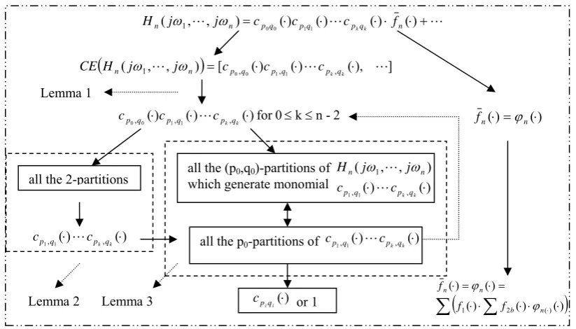
Figure 1. An illustration of the relationships in Proposition 1 To further demonstrate the result in Proposition 1, the following example is given.

Example 1. Consider the 4th-order GFRF. The parametric characteristic of the 4th-order GFRF can be obtained from Lemma 1 that

(

H₄(jω₁, ,jω₄)

)

CE L = C0,4⊕C1,3⊕C3,1⊕C2,2⊕C4,0⊕C1,1⊗C0,3⊕C1,1⊗C1,2

⊕C1,1⊗C2,1⊕C1,1⊗C3,0⊕C1,2⊗C0,2⊕C1,2⊗C2,0 ⊕C2,0⊗C0,3 ⊕ C2,0⊗C2,1⊕C2,0⊗C3,0⊕ C2,1⊗C0,2⊕C3,0⊗C0,2

⊕ C1,1⊗C0,22⊕C1,12⊗C0,2⊕C1,1⊗C0,2⊗C2,0⊕ C1,13⊕C1,12⊗C2,0 ⊕C1,1⊗C2,02⊕C2,0⊗C0,22⊕C2,02⊗C0,2⊕C2,03 By using Proposition 1, the correlative function of each term in CE

(

H4(jω1,L,jω4)

)

can all be obtained. For example, for the term c1,1(.)c0,2(.)c2,0(.), it can be derived that

[

]

[

]

) ); ) ( ( ( ) ); ) ( ( ( ) ); ) ( ) ( ( ( ) ); ) ( ) ( ( ( ) ); ) ( ) ( ( ( ) ); ) ( ) ( ( ( ) ; 4 ), ( ( ) ); ) ( ) ( ( ( ) ); ) ( ) ( ( ( ) ; 4 ), ( ( ) ); ( ) ( ) ( ( ) ); ( ) ( ) ( ( ) ) ) ( ( ( ) 2 ( 1 ) 2 ( 2 , 0 1 ) ) ) ( ( ( ) ) ) ( ( ( ) 1 ( 1 ) 1 ( 1 , 1 1 ) ) ) ( ( ( 4 1 2 , 0 1 , 1 1 1 2 ) ) ) ( ) ( ( ( ) 2 ( 1 ) 2 ( 2 , 0 1 , 1 2 ) ) ) ( ) ( ( ( ) ) ) ( ) ( ( ( ) 1 ( 1 ) 1 ( 2 , 0 1 , 1 0 ) ) ) ( ) ( ( ( 4 1 2 , 0 1 , 1 2 0 2 4 1 0 , 2 1 ) ) ) ( ) ( ( ( ) 1 ( 1 ) 1 ( 0 , 2 2 , 0 2 ) ) ) ( ) ( ( ( 3 1 0 , 2 2 , 0 2 2 4 1 1 , 1 1 4 1 0 , 2 2 , 0 1 , 1 4 )) ( ( ) 1 ( 0 , 2 2 , 0 1 , 1 ) ( 2 , 0 1 2 , 0 1 1 , 1 1 1 , 1 1 2 , 0 1 , 1 2 2 , 0 1 , 1 2 2 , 0 1 , 1 0 2 , 0 1 , 1 0 0 , 2 2 , 0 2 0 , 2 2 , 0 2 ⋅ + + ⋅ ⋅ + + ⋅ ⋅ ⋅ + + ⋅ ⋅ ⋅ ⋅ + + ⋅ ⋅ ⋅ ⋅ + + ⋅ ⋅ ⋅ ⋅ ⋅ ⋅ ⋅ ⋅ + ⋅ ⋅ ⋅ ⋅ ⋅ ⋅ ⋅ ⋅ ⋅ ⋅ + ⋅ ⋅ ⋅ ⋅ ⋅ ⋅ ⋅ = ⋅ ⋅ ⋅ = ⋅ ⋅ ⋅ c s n X X c s n c s n X X c s n b c c s n X X c c s n c c s n X X c c s n b c c s n X X c c s n b s n l l s n c s c s c c s s f c c s c c s c c s s f c f c c s c c s f c f c c c c c c ω ω ϕ ω ω ϕ ω ω ω ω ϕ ω ω ϕ ω ω ω ω ω ω ϕ ω ω ω ω ω ω ϕ ω ω ϕ L L L L L L L L L L L L

(

( ₁, , )

)

[ _, () _, () _, (), ]

1 1 0

0 L L

L n = p q ⋅ p q ⋅ p_kq_k ⋅

n j j c c c

H

CE ω ω

2 -n k 0 for ) ( ) ( ) ( _{, ,}

, 0 1 1

0q ⋅ p q ⋅ pkqk ⋅ ≤ ≤

p c c

c L

all the 2-partitions all the (p_{which generate monomial} 0,q0)-partitions of

) , ,

( _{1 n}

n j j

H ω L ω ) ( )

( _,

,1

1q ⋅ pkqk ⋅

p c

c L

all the p0-partitions of

or 1piqi(⋅)

c

Lemma 2 Lemma 3

Lemma 1

) ( ) (⋅ = _n ⋅ n f ϕ

(

)

∑

⋅ ⋅

∑

⋅ ⋅ ⋅ = ⋅ = ⋅ ⋅() ) ( ) ( ) ( ) ( ) ( 2

1 b n

n n f f f ϕ ϕ L L

L, )= (⋅) (⋅) (⋅)⋅ (⋅)+ , ( 1 1 0 0

1 n pq pq pq n

n j j c c c f

H k k ω ω ) ( ) ( , ,1

1q ⋅ pkqk ⋅

p c

c L _, () _, ()

1

1q ⋅ pkqk ⋅

p c

[

]

[

]

[

]

[

]

(22)

) , ; ) ( ( ) , ; ) ( ( ) ); ) ( ) ( ( ( ) ; ) ( ) ( ( ) ; 1 ( ) ); ) ( ) ( ( ( ) ; 4 ), ( ( ) ; ) ( ) ( ( ) ; ) ( ) ( ( ) ; 4 ), ( ( ) ; ) ( ( ) ; ) ( ( ) ); ) ( ) ( ( ( ) ; ) ( ) ( ( ) ; 1 ( ) ); ) ( ) ( ( ( ) ; 4 ), ( ( ) ; ) ( ) ( ( ) ; ) ( ) ( ( ) ; 4 ), ( ( 4 3 2 , 0 2 2 1 1 , 1 2 4 1 2 , 0 1 , 1 1 1 2 4 2 2 , 0 1 , 1 3 1 1 4 1 2 , 0 1 , 1 2 0 2 4 1 0 , 2 1 3 1 0 , 2 2 , 0 3 3 1 0 , 2 2 , 0 2 4 1 1 , 1 1 ) ) ) ( ( ( ) 2 ( 1 ) 2 ( 2 , 0 2 ) ) ) ( ( ( ) 1 ( 1 ) 1 ( 1 , 1 2 4 1 2 , 0 1 , 1 1 1 2 )) ( ) ( ( ) 1 ( 1 ) 1 ( 2 , 0 1 , 1 )) ( ) ( ( ) 1 ( 1 ) 1 ( 4 1 2 , 0 1 , 1 2 0 2 4 1 0 , 2 1 )) ( ) ( ( 0 1 0 0 , 2 2 , 0 )) ( ) ( ( 3 1 0 , 2 2 , 0 2 4 1 1 , 1 1 2 , 0 1 1 , 1 1 2 , 0 1 , 1 2 , 0 1 , 1 0 , 2 2 , 0 0 , 2 2 , 0 ω ω ϕ ω ω ϕ ω ω ω ω ϕ ω ϕ ω ω ω ω ω ω ϕ ω ω ω ω ω ω ϕ ω ω ϕ ω ω ω ω ϕ ω ω ϕ ω ω ω ω ω ω ϕ ω ω ω ω ⋅ ⋅ ⋅ ⋅ ⋅ ⋅ + ⋅ ⋅ ⋅ ⋅ ⋅ ⋅ ⋅ + ⋅ ⋅ ⋅ ⋅ ⋅ ⋅ ⋅ = ⋅ ⋅ ⋅ ⋅ ⋅ ⋅ + ⋅ ⋅ ⋅ ⋅ ⋅ ⋅ ⋅ + ⋅ ⋅ ⋅ ⋅ ⋅ ⋅ ⋅ = ⋅ + + ⋅ + + ⋅ ⋅ + + ⋅ ⋅ ⋅ ⋅ + + ⋅ ⋅ c c c c s s f c c c c s s f c f c c c c f c f c c c c s s f c c c c s s f c f c c c c f c f b b b c s n X X c s n X X b c c n n n c c n n n b c c n c c n b L L L L L L L L L L L L L L L L L

To proceed with the recursive computation, it can be derived that ) ( ) ( ) ( ) ( ) ; 4 ), ( ( 4 1 4 4 4 1 4 1 1 3 4 1 1 , 1 1 2

1

∑

∑

∏

= = = + = = ⋅ + i i k i i i k

i L j j L j

j c

f ω Lω ω i ω ω ω (23a)

) ( 1 ) ; 4 ), ( ( 4 1 4 4 1 0 , 2 1

∑

= = ⋅ i i j L c

f ω Lω ω (23b) 1

1( () ()); ) ( )

( _{2,0 0,2 1 3 1 3}

2

k x

b s c c j j

f ⋅ ⋅ ω Lω = ω +L+ ω (23c)

2 1 2 1 1 ) ( ) ( ) ( ) ( ) ( ) ); ) ( ) ( ( ( 1 4 2 4 2 1 } , , { of ns permutatio different the all 2 1 ))) ( / ( ( ) ( 1 ) ( 4 1 2 , 0 1 , 1 2 0 2 k k k k k k i k c s s n i X i X b j j j j j j j j c c s s f p i pq i x ω ω ω ω ω ω ω ω ω ω + + + + + = + + = ⋅ ⋅

∑ ∏

= ⋅ + + L L L L

L (23d)

(

)

) 23 ( ) ( ) ( ) ( 1 ) ( ) ( ) ( ) ( ) ( ) ( 1 ) , ; ) ( ( ) ; 1 ( ) ); ) ( ( ( ) ; 3 ), ( ( ) ); ) ( ( ( ) ); ) ( ( ( ) ; 3 ), ( ( ) ; ) ( ) ( ( 2 1 2 1 2 1 2 1 2 , 0 2 1 3 2 3 2 2 1 1 1 2 3 3 2 1 3 1 3 3 2 2 , 0 2 1 1 3 1 2 , 0 2 3 1 0 , 2 1 2 1 ) ) ) ( ( ( ) ( 1 ) ( 2 , 0 ) ) ) ( ( ( 3 1 2 , 0 2 3 1 0 , 2 1 3 1 0 , 2 2 , 0 3 e j j j j L j H j j j j j j j L c c s s f c f c s c s s f c f c c k k k k k k i i x x b i c s n i X i X x c s s n x x

b xi pq i x_i

ω ω ω ω ω ω ω ω ω ω ω ω ω ω ϕ ω ϕ ω ω ω ω ω ω ϕ ω ω ω ω ω ω ϕ + ⋅ ⋅ + + + ⋅ = ⋅ ⋅ ⋅ ⋅ = ⋅ ⋅ ⋅ ⋅ = ⋅ ⋅

∑

∏

= = ⋅ + + ⋅ L L L L L L 2 1 1 2 1 2 , 0 1 1 ) ( ) ( ) ( 1 ) ( ) ( ) ( ) , ; ) ( ( ) , ; ) ( ( ) ; 3 ), ( ( ) , ); ) ( ( ( ) , ); ) ( ( ( ) ; 3 ), ( ( ) ; ) ( ) ( ( 3 2 3 2 2 3 2 4 2 3 4 3 2 2 , 0 2 3 2 2 , 0 2 4 2 1 , 1 1 3 2 2 , 0 ) ) ) ( ( ( 3 2 2 , 0 2 4 2 1 , 1 1 4 2 2 , 0 1 , 1 3 k k k k b x c s n x b j j j j L j j j j L j c c f c f c s c s f c f c c x ω ω ω ω ω ω ω ω ω ω ω ϕ ω ω ω ω ω ω ϕ ω ω ω ω ω ω ϕ + ⋅ + ⋅ + + = ⋅ ⋅ ⋅ ⋅ ⋅ = ⋅ ⋅ ⋅ ⋅ ⋅ = ⋅ ⋅ ⋅ L L L L (23f)

[

]

[

]

(

)

(

)

(

)

_{( )} ) ( ) ( ) ( ) ( ) ( ) ( ) ( ) ( ) ( ) ( ) ( ) ( ) ( ) ( ) ( ) ( ) ( ) ( ) ( ) ( ) ( ) ( ) ( ) ( ) ( ) ( ) ( ) ( ) ( ) ( ) ( ) ( ) ( ) ( ) ( ) , ; ) ( ( ) , ; ) ( ( ) ); ) ( ) ( ( ( ) ; ) ( ) ( ( ) ; 1 ( ) ); ) ( ) ( ( ( ) ; 4 ), ( ( ) ; ) ( ) ( ( ) ; ) ( ) ( ( ) ; 4 ), ( ( ) ); ( ) ( ) ( ( 1 1 1 2 2 4 3 2 4 1 4 2 1 3 4 2 1 4 3 4 3 2 1 1 1 3 2 2 4 2 3 4 1 4 3 2 3 2 4 1 4 2 4 2 1 1 1 3 2 2 3 2 1 3 4 1 4 3 2 1 2 3 3 2 1 3 1 4 4 3 2 , 0 2 2 1 1 , 1 2 4 1 2 , 0 1 , 1 1 1 2 4 2 2 , 0 1 , 1 3 1 1 4 1 2 , 0 1 , 1 2 0 2 4 1 0 , 2 1 3 1 0 , 2 2 , 0 3 3 1 0 , 2 2 , 0 2 4 1 1 , 1 1 4 1 0 , 2 2 , 0 1 , 1 4 2 1 1 2 2 1 2 1 2 1 1 2 2 1 2 1 2 1 2 1 2 1 1 2 ω ω ω ω ω ω ω ω ω ω ω ω ω ω ω ω ω ω ω ω ω ω ω ω ω ω ω ω ω ω ω ω ω ω ω ω ω ω ω ω ω ω ω ω ω ω ω ω ω ω ω ω ω ω ω ω ω ω ϕ ω ω ϕ ω ω ω ω ϕ ω ϕ ω ω ω ω ω ω ϕ ω ω ω ω ω ω ϕ j H j j L j j L j j L j j j j j j j j j j j j j H j j L j j L j j L j j j j j j j j j j j j H j j L j j j L j j L j j j j j j j j j j j c c c c s s f c c c c s s f c f c c c c f c f c c c k k k k k k k k k k k k k k k k k k k k k k k k b b b + + + + + + + + + + + + + + + + + + + + + + ⋅ + + + + + + + + + + = ⋅ ⋅ ⋅ ⋅ ⋅ ⋅ + ⋅ ⋅ ⋅ ⋅ ⋅ ⋅ ⋅ + ⋅ ⋅ ⋅ ⋅ ⋅ ⋅ ⋅ = ⋅ ⋅ ⋅ L L L L L L L L L L L L L L L (24) Therefore, the correlative function of the parameter monomial c_1,1(⋅)c_0,2(⋅)c_2,0(⋅)is obtained. It can be verified that the same result can be obtained by using the recursive algorithm in (12, 5-7, 11). For the sake of brevity, this is omitted. By following the same method, the whole correlative function vector ϕ₄

(

CE

(

H₄(jω₁,L,jω₄)

)

)

can be determined. Thus the 4th -order GFRF H₄(jω₁,L,jω₄)can directly be written into a parametric characteristic form which can provide a straightforward and meaningful insight into the relationship between

) , ,

( _{1 4}

4 jω jω

H L and nonlinear parameters, and also between H₄(jω₁,L,jω₄)andH₁(jω₁).

Remark 3. From Example 1, it can be seen that Proposition 1 provides an effective method to determine the correlative function for an effective monomial

) ( ) ( ) ( , ,

,0 1 1

0q ⋅ p q ⋅ pkqk ⋅

p c c

c L , and the computation process should be able to be carried out automatically without manual intervention. Therefore, Proposition 1 provides a simplified method to determine the nth-order GFRF directly into a more meaningful form as (14) which can demonstrate the parametric characteristic clearly and describe the n th-order GFRF in terms of the first th-order GFRFH1(jω)and nonlinear parameters without crossing effect with the lower order GFRFs. This reveals a more straightforward insight into the relationships between H_n(jω₁,L,jω_n) and nonlinear parameters, and between

) , ,

( _{1 n}

n j j

H ω L ω and H₁(jω) . Note that the high order GFRFs can represent system frequency response characteristics (Peyton Jones and Billings 1990, Yue et al 2005) and

) (

1 jω

H represents the linear part of the system model. Hence, the results in Proposition 1 not only facilitate the analysis of the connection between system frequency response characteristics and model linear and nonlinear parameters, but also provide a new perspective on the understanding of the GFRFs and on the analysis of nonlinear systems based on the GFRFs.

4 Some new properties

Based on the mapping function ϕn established in the last section, some new properties of

the nth-order GFRF are discussed in this section.

4.1 Determination of FRFs based on parametric characteristics

There are several relationships involved in this paper. H_n(jω₁,L,jω_n)is determined from the NDE model in terms of the model parameters. Thus there is a bijective mapping between Hn(jω1,L,jωn) and the NDE model. The CE operator is a mapping from

) , ,

( _{1 n}

n j j

H ω L ω to its parametric characteristic, which can also be regarded as a mapping from the nonlinear parameters of the NDE model to the parametric characteristics of

) , ,

( _{1 n}

n j j

H ω L ω . The function ϕn can be regarded as an inverse mapping of the CE

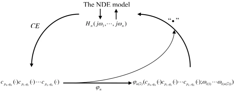
operator such that the nth-order GFRF can be reconstructed from its parametric characteristic, which can also be regarded as a mapping from the nonlinear parameters of the NDE model to H_n(jω₁,L,jω_n). This can refer to Figure 2, where “•” represents the point multiplication between the parametric monomial and its correlative function.

It can be seen from Figure 2 that

))) ( ( ( )) ( ( ) , ,

( _{1 n} = _n ⋅ ⋅ _{n n} ⋅

n j j CE H CE H

H ω L ω ϕ (25) From (25), the inverse of the operator CE can simply be written as (x=CE(Hn(⋅)))

) ( )

(

1

x x x

CE = ⋅ϕn

−

which constructs a mapping directly from the parametric characteristic of the nth-order GFRF to the nth-order GFRF itself. Note that CE(H_n(⋅)) includes all the nonlinear parameters of degree from 2 to n of the nonlinear system of interest, and ϕ_n(CE(H_n(⋅)))is a complex valued function vector including the effect of the complicated nonlinear behaviour and also the effect of the linear part of the nonlinear system. Hence, Equation (25) reveals a new perspective on the computation and understanding of the GFRFs as discussed in Section 3, and also provides a new insight into the frequency domain analysis of nonlinear systems based on the GFRFs.

From the results in Jing et al (2006), the output spectrum for system (1) can now be determined as

(

)

∑

=

⋅ = N

n

n n

n j j F j

H CE j

Y

1

1, , ) ˆ ( )

( )

( ω ω L ω ω (26a) when the input is a general input U(jω),

) );

( ) ( ) (

( _{, , , (1) (())}

)

(s p0q0 p1q1 p q l lns

n c c c k k ω ω

ϕ ⋅ ⋅L ⋅ L

) ( )

( )

( _{, ,}

,0 1 1

0q ⋅ p q ⋅ pkqk ⋅

p c c

c L

n ϕ

[image:17.595.88.475.268.420.2]

CE Hn(jω1,L,jωn) “•”

Figure 2. Relationship between ϕn and CE