C2-Element radial basis function methods for some continuum mechanics problems

(1)

UNIVERSITY OF SOUTHERN QUEENSLAND

C

2

-ELEMENT RADIAL BASIS FUNCTION

METHODS FOR SOME CONTINUUM MECHANICS

PROBLEMS

A dissertation submitted by

DUC-ANH AN-VO

B.Eng. (Hon.), Ho-Chi-Minh City University of Technology, Vietnam, 2005

M.Sc. (Hon.), Toyohashi University of Technology, Japan, 2007

For the award of the degree of

Doctor of Philosophy

(2)

Dedication

To my parents

Thanh Vo-Kim and Dung An-Bang

and

The woman in my life

(3)

Certification of Dissertation

I certify that the ideas, experimental work, results and analyses, software and

conclusions reported in this dissertation are entirely my own effort, except where

otherwise acknowledged. I also certify that the work is original and has not been

previously submitted for any other award.

Duc-Anh An-Vo, Candidate Date

ENDORSEMENT

Prof. Nam Mai-Duy, Principal supervisor Date

Prof. Thanh Tran-Cong, Co-supervisor Date

(4)

Acknowledgments

I would like to acknowledge my supervisors Professor Nam Mai-Duy, Professor Thanh Tran-Cong and Dr Canh-Dung Tran for their effective guidance, constant support and encouragement throughout. I deeply appreciate their knowledge and patience to answer any question I have asked and correct my manuscripts. They are indeed wonderful supervisors.

In addition, I would like to thank A/Prof. Armando A. Apan, Mrs Juanita Ryan (Faculty of Engineering and Surveying), Ms Katrina Hall (Office of Research and Higher Degrees), Mr Martin Geach (P9 operational officer) for their kind support; Dr Andrew Wandel and Dr Kazem Ghabraie for offering me teaching assistant positions.

I am grateful to numerous friends and people, whom I have not mentioned by name, for their invaluable help during the course of my study.

My candidature was at all possible owing to a Postgraduate Scholarship from the University of Southern Queensland and Scholarship supplements from Fac-ulty of Engineering and Surveying and Computational Science and Engineering Research Centre. These financial supports are gratefully acknowledged.

(5)

Abstract

This work attempts to contribute further knowledge to high-order approxima-tion and associated advanced techniques/methods for the numerical soluapproxima-tion of differential equations in the discipline of computational science and engineering. Of particular interest is the numerical simulation of heat conduction, highly non-linear flows and multiscale problems. The distinguishing feature in this study is the development of novel local compact 2-node integrated radial basis function elements (IRBFEs) and their incorporation into the subregion/point collocation formulations based on Cartesian grids. As a result, a new class of C2_{-continuous methods are devised, representing a significant improvement}

on the usual C0_{-continuous methods. Incorporation of the new} _C2_-continuous

methods into the development of a high-order multiscale computational frame-work provides advantageous features compared to other multiscale frameframe-works available in the literature, including (i) high rates of convergence and levels of accuracy; and (ii) converged C2_{-continuous solutions of two-dimensional}

multi-scale elliptic problems.

Firstly, a new control-volume (CV) discretisation method, based on Cartesian grid and IRBFEs, for solving PDEs is proposed. Unlike the standard CV method (Patankar 1980), the flux values at CV faces are presently estimated with high-order IRBF approximations on 2-node elements and the solution is C2_{-continuous across the interface between two adjacent elements. Only two}

(6)

Abstract v

used to effectively control the solution accuracy. Secondly, the proposed 2-node IRBFEs are incorporated into the subregion and point collocation frameworks for the discretisation of the streamfunction-vorticity formulation governing the fluid flows. Several high-order upwind schemes based on 2-node IRBFEs are de-veloped for highly non-linear flows. Thirdly, the ADI procedure (Peaceman and Rachford 1955, Douglas and Gunn 1964) is applied to enhance the efficiency of the proposed methods. Especially novel C2_{-continuous compact schemes}

based on 2-node IRBFEs are devised and combined with the ADI procedure to yield optimal tridiagonal system matrices on each and every grid line. Such tridiagonal matrices can be solved effectively and efficiently with the Thomas algorithm (Fletcher 1991, Pozrikidis 1997). Finally, the proposedC2_-continuous

CV method is employed in a multiscale basis function approach to develop a high-order multiscale CV method for the solution of multiscale elliptic problems.

(7)

Papers Resulting from the

Research

Journal Papers

1. D.-A. An-Vo, N. Mai-Duy, T. Tran-Cong (2010). Simulation of Newtonian-fluid flows with C2_{-continuous two-node integrated-RBF elements,} _SL:

Structural Longevity, 4(1):39 – 45.

2. D.-A. An-Vo, N. Mai-Duy, T. Tran-Cong (2011). A C2_-continuous

control-volume technique based on Cartesian grids and two-node integrated-RBF elements for second-order elliptic problems. CMES: Computer Mod-eling in Engineering and Sciences, 72(4):299 – 335.

3. D.-A. An-Vo, N. Mai-Duy, T. Tran-Cong (2011). High-order upwind methods based on C2_{-continuous two-node integrated-RBF elements for}

viscous flows. CMES: Computer Modeling in Engineering and Sciences, 80(2):141 – 177.

4. C.-D. Tran, D.-A. An-Vo, N. Mai-Duy, T. Tran-Cong (2011). An inte-grated RBFN based macro-micro multi-scale method for computation of visco-elastic fluid flows. CMES: Computer Modeling in Engineering and Sciences, 82(2):137 – 162.

(8)

Papers Resulting from the Research vii

method based on C2_{-continuous two-node integrated-RBF elements for}

viscous flows. Applied Mathematical Modelling, 37:5184 – 5203.

6. D.-A. An-Vo, C.-D. Tran, N. Mai-Duy, T. Tran-Cong (2013). RBF-based multiscale control volume method for second order elliptic problems with oscillatory coefficients. CMES: Computer Modeling in Engineering and Sciences, Accepted 21/01/2013.

7. D.-A. An-Vo, N. Mai-Duy, C.-D. Tran, T. Tran-Cong (2013). A C2

-continuous compact implicit method for parabolic equations, submitted.

Conference Papers

1. D.-A. An-Vo, D. Ngo-Cong, B.H.P Le, N. Mai-Duy, T. Tran-Cong (2010). Local integrated radial-basis-function discretisation schemes. The ICCES Special Symposium on Meshless & Other Novel Computational

Methods (ICCES-MM’10), 17-21/Aug/2010, Busan, Korea Republic. IC-CES Journal, Tech Science Press (ISSN 1933-2815).

2. D.-A. An-Vo, N. Mai-Duy, T. Tran-Cong (2011). IRBFEs for the nu-merical solution of steady incompressible flows. ICCES: International Conference on Computational & Experimental Engineering and Sciences, 16(3) 87 – 88, 2011.

3. D.-A. An-Vo, C.-D. Tran, N. Mai-Duy, T. Tran-Cong (2011). IRBFN-based multiscale solution of a model 1D elliptic equation. In Boundary Element and Other Mesh Reduction Methods XXXIII, 241 – 251. ISSN 1743-355X (invited).

(9)

Papers Resulting from the Research viii

fluid flows. The 1st _{International Conference on Computational Science}

and Engineering, 19-21/Dec/2011, HCM city, Vietnam (invited).

5. D.-A. An-Vo, N. Mai-Duy, C.-D. Tran, T. Tran-Cong (2012). Model-ing strain localisation in a segmented bar by a C2_{-continuous two-node}

integrated-RBF element formulation. In Boundary Element and Other Mesh Reduction Methods XXXIV, 3 – 13. ISSN 1743-3533 (invited).

(10)

Acronyms & Abbreviations

1D-IRBF One-dimensional Integrated Radial Basis Function 2D-IRBF Two-dimensional Integrated Radial Basis Function ADI Alternating Direction Implicit

BEM Boundary Element Method

C2NIRBFM Compact 2-node Integrated Radial Basis Function Method CD Central Difference

CFD Computational Fluid Dynamics CM Collocation Method

CM Convergence Measure

CPU Central Processing Unit

CV Control Volume

CVM Control Volume Method

DGM Discontinuous Galerkin Method DRBF Differentiated Radial Basis Function ETCM Explicit Treatment of Convection Method FD Finite Difference

FDM Finite Difference Method

FE Finite Element

(17)

Acronyms & Abbreviations xvi

HMM Heterogeneous Multiscale Method HOC High-Order Compact

IRBF Integrated Radial Basis Function

IRBFE Integrated Radial Basis Function Element LCR Local Convergence Rate

LHS Left Hand Side LR Line Relaxation MD Multidomain

MFEM Multiscale Finite Element Method MFVM Multiscale Finite Volume Method MHM Mathematical Homogenisation Method MQ Multiquadric

N-S Navier-Stokes

ODE Ordinary Differential Equation PDE Partial Differential Equation PR Peaceman and Rachford RBF Radial Basis Function RHS Right Hand Side

SVD Singular Value Decomposition

(18)

List of Tables

2.1 List of semi-interior elements and their characteristics. . . 33

2.2 ODE, Problem 1, Dirichlet boundary conditions: rates of con-vergence O(hα_{) for} _φ _and _∂φ/∂x _{for several large} _β _{values and}

semi-interior element types. . . 45

2.3 ODE, Problem 1, Dirichlet-Neumann boundary conditions: rates of convergence O(hα_{) for}_φ _and _∂φ/∂x _{for two semi-interior}

ele-ment types. . . 45

2.4 ODE, Problem 2, Dirichlet boundary conditions: rates of con-vergence O(hα_{) for} _φ _and _∂φ/∂x _{for several} _β _{values and}

semi-interior element types. . . 46

2.5 ODE, Problem 2, Dirichlet and Neumann boundary conditions,

D3-N2 treatment: rates of convergence O(hα_{) for} _φ _and _∂φ/∂x

for several β values. . . 46

2.6 PDE, Problem 1 and Problem 2: Rates of grid convergence O(hα_{) for the field variable and its first-order partial derivatives,}

(19)

List of Tables xviii

3.1 Lid-driven cavity flow, IRBFE-CVM, Re = 100: extrema of ve-locity profiles on the vertical and horizontal centrelines of the cavity. [⋆] is Ghia et al. (1982) and [⋆⋆] is Botella and Peyret (1998). . . 79

3.2 Lid-driven cavity flow, IRBFE-CVM,Re= 1000: extrema of the vertical and horizontal velocity profiles through the centrelines of the cavity. [⋆] is Ghia et al. (1982) and [⋆⋆] is Botella and Peyret (1998). . . 80

3.3 Lid-driven cavity flow, IRBFE-CVM, Re= 1000: percentage er-rors relative to the spectral benchmark results for the extreme values of the velocity profiles on the centrelines. Results of up-wind central difference (UW-CD), central difference (CD-CD) and global 1D-IRBF-CVM are taken from Mai-Duy and Tran-Cong (2011a). . . 81

3.4 Lid-driven cavity flow, IRBFE-CM, Re = 1000: effects of β on the solution accuracy. The present results at the “optimal” value (i.e. about 3) with a grid of 51_×51 are in better agreement with the benchmark spectral results than those by 1D-IRBF-CM using the same grid and by FDM using a much denser grid. [⋆] is Mai-Duy and Tran-Cong (2009b), [⋆⋆] is Ghia et al. (1982), and [⋆ ⋆ ⋆] is Botella and Peyret (1998). . . 82

3.5 Flow past a circular cylinder in a channel, IRBFE-CVM, γ = 0.5: The critical Reynolds numberRecritfor the formation of the

(20)

List of Tables xix

3.6 Flow past a circular cylinder in a channel, γ = 0.5, Re = 60: minimum velocity umin and its position on the centreline, and

the length of recirculation zones behind the cylinder (Lw). It is

noted that the case of Re= 60 and γ = 0.5 here is equivalent to the case ofRe= 45 and γ = 0.5 in Singha and Sinhamahapatra (2010). . . 91

4.1 Square cavity flow: computational times. . . 113

4.2 Square cavity flow: extrema of the vertical and horizontal veloc-ity profiles along the centrelines of the cavveloc-ity. % denotes per-centage errors relative to the benchmark spectral results (Botella and Peyret 1998). Results of the global 1D-IRBF-C, FDM and Benchmark are taken from Mai-Duy and Tran-Cong (2009b), Ghia et al. (1982) and Botella and Peyret (1998) respectively. . 115

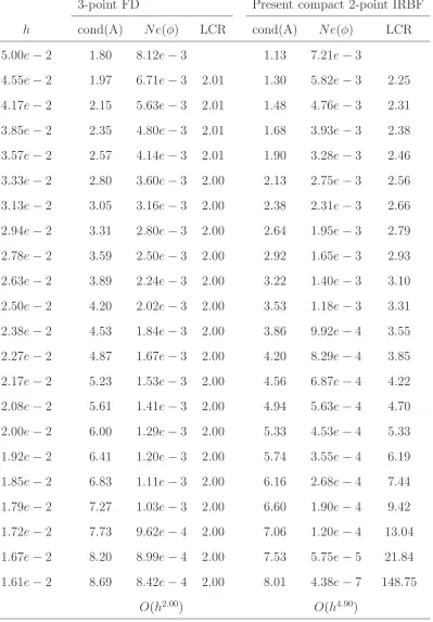
5.1 One-dimensional problem, Dirichlet boundary conditions only, N = (21,23, . . . ,63), ∆t = 0.001: condition numbers of the sys-tem matrix and relative L2 errors of the approximate solution φ

att= 1 for various values ofhby the 3-point FD method and the present compact 2-point IRBF method (β = 231). LCR stands for local convergence rate. . . 148

5.2 One-dimensional problem, Dirichlet and Neumann boundary con-ditions, N = (21,23, . . . ,63), ∆t = 0.001: condition numbers of the system matrix and relativeL2 errors of the approximate

(21)

List of Tables xx

5.3 Rectangular domain problem, Dirichlet boundary conditions only, Nx×Ny = (21×21,23×23, . . . ,63×63), ∆t = 0.001:

condi-tion numbers of the system matrix on a grid line and relativeL2

errors of the approximate solution φ at t = 1 for various values ofh by the 3-point FD method and the present compact 2-point IRBF method (β = 124). LCR stands for local convergence rate. 155

5.4 Circular domain problem, Nx×Ny = (21×21,23×23, . . . ,51×

51), ∆t = 0.001: maximum condition numbers of the system matrix on a grid line and relative L2 errors of the approximate

solution φ at t = 0.05 for various values of h by the present compact 2-point IRBF method (β = 330). LCR stands for local convergence rate. . . 161

5.5 Lid-driven cavity flow: extrema of the vertical and horizontal ve-locity profiles along the centrelines of the cavity. % denotes per-centage errors relative to the benchmark spectral results (Botella and Peyret 1998). Results of the FDM are taken from Ghia et al. (1982). . . 172

6.1 One-dimensional example 1, ε = 0.01, Strategy 1: L2 errors of

the field variable, its first and second derivatives. It is noted that the set of test nodes contains 10,001 uniformly distributed points. LCR stands for local convergence rate. . . 216

(22)

List of Tables xxi

the field variable, its first and second derivatives by the present method. It is noted that the set of test nodes contains 100,001 uniformly distributed points. LCR stands for local convergence rate. . . 221

the field variable, its first and second derivatives by the present method. It is noted that the set of test nodes contains 100,001 uniformly distributed points. LCR stands for local convergence rate. . . 222

6.5 Two-dimensional example 1: L2 errors of the field variable, its

first and second derivatives. LCR stands for local convergence rate. . . 227

6.6 Two-dimensional example 2, ε= 0.1: L2 errors of the field

vari-able, its first and second derivatives. LCR stands for local con-vergence rate. . . 235

6.7 Two-dimensional example 2, ε = 0.01: L2 errors of the field

(23)

List of Figures

1.1 Exact solution of problem (1.22)-(1.24) for ǫ = 0.01: (a) field variable, (b) its zoomed part, (c) its first-order derivative, (d) its second-order derivative. . . 14

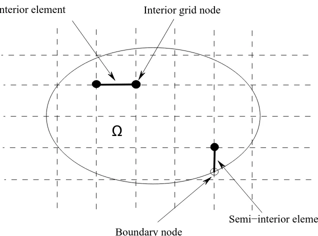
2.1 A domain is embedded in a Cartesian grid with interior and semi-interior elements. . . 28

2.2 Schematic outline for 2-node IRBFE. . . 29

2.3 Schematic outline for a control volume in 2D. . . 34

2.4 Function approximation: Approximation for functions (left) and their first-order derivative (right) by using one IRBFE only. It can be seen that the present two-node IRBFE is able to produce non-linear behaviours (i.e. curved lines) between the two extremes. 40

2.5 Function approximation (continued), trigonometric function: Ap-proximations for the function (left) and its first-order derivative (right). . . 41

(24)

List of Figures xxiii

2.7 ODE, Problem 1, Dirichlet boundary conditions,n= 9: Compar-ison of the exact and approximate solutions for φ and dφ/dxby the present D1-D1 strategy (left) and the standard CV method (right). . . 43

2.8 ODE, Problem 1, Dirichlet boundary conditions: h-adaptivity studies conducted with several values ofβfor theD1-D1 strategy. It is noted that results with β = (5,10,15) are undistinguishable. 44

2.9 ODE, Problem 1, Dirichlet boundary conditions: Effects of types of semi-interior elements on the solution accuracy for β = 15. . . 44

2.10 ODE, Problem 1, Dirichlet boundary conditions: β-adaptivity studies conducted withn = 9 (left) andn= 153 (right) for three boundary treatment strategies. . . 47

2.11 ODE, Problem 1, Dirichlet and Neumann boundary conditions: Effects of types of semi-interior elements on the solution accu-racy for β = 1 (left) and β = 15 (right). It is noted that plots have the same scaling and results by the two boundary treatment strategies are undistinguishable. . . 48

2.12 ODE, Problem 2: Exact solution (a) and its first-order derivative (b). . . 49

2.13 ODE, Problem 2, Dirichlet boundary conditions: h-adaptivity studies conducted with β = 1 (left) and β = 15 (right). . . 50

(25)

List of Figures xxiv

2.15 ODE, Problem 2, Dirichlet and Neumann boundary conditions: h-adaptivity (left) andβ-adaptivity (right) studies for theD3-N2

strategy. . . 51

2.16 Half control volume associated with a boundary node in 2D. . . 51

2.17 PDE, Problem 1, rectangular domain, Dirichlet boundary con-ditions: h-adaptivity studies for the D1-D1 (left) and D2-D2

(right) strategies. . . 52

2.18 PDE, Problem 1, rectangular domain, Dirichlet and Neumann boundary conditions: h-adaptivity studies conducted withβ = 1 and β = 15 for the D1-N2 strategy. . . 53

2.19 PDE, Problem 2: Geometry and discretisation. Boundary nodes denoted by _◦ are generated by the intersection of the grid lines and the boundary. . . 57

2.20 PDE, Problem 2, circular domain, Dirichlet boundary conditions: the solution accuracy using theD1-D1 strategy and β = 15. . . 58

3.1 Lid-driven cavity flow, IRBFE-CVM, Re= 1000, grid = 81_×81, solution at Re = 400 used as initial guess: convergence be-haviour. Scheme 1 using a time step of 3_×10−4 _converges

re-markably faster than the no-upwind version using a time step of 7_×10−6_{. It is noted that the latter diverges for time steps greater}

than 7_×10−6_. _CM _{denotes the convergence measure as defined}

(26)

List of Figures xxv

3.2 Lid-driven cavity flow, IRBFE-CM, Re= 1000, grid = 81_×81, solution at Re = 400 used as initial guess: convergence be-haviour. Scheme 2 and Scheme 3, using a time step of 3_×10−4

and 10−4_{, respectively, converge remarkably faster than the}

no-upwind version using a time step of 8_×10−6_{. It is noted that the}

latter diverges for time steps greater than 8_×10−6_. _CM _denotes

the convergence measure as defined by (3.38). . . 75

3.3 Lid-driven cavity flow, IRBFE-CVM, Re= 3200, grid = 91_×91, solution at Re = 2000 used as initial guess: convergence be-haviour. Scheme 1 using a time step of 10−4_{converges remarkably}

faster than the no-upwind version using a time step of 8_×10−7_.

It is noted that the latter diverges for time steps greater than 8_×10−7_. _CM _{denotes the convergence measure as defined by}

(3.38). . . 76

3.4 Lid-driven cavity flow, IRBFE-CVM: velocity profiles on the ver-tical (left) and horizontal (right) centrelines at different grids, results by Ghia et al. (1982) were obtained at a grid of 129_×129. [_∗] is Ghia et al. (1982) and [_∗∗] is Botella and Peyret (1998). . 83

3.5 Lid-driven cavity flow, IRBFE-CVM: velocity profiles on the ver-tical (left) and horizontal (right) centrelines at different grids, results by Ghia et al. (1982) were obtained at a grid of 129_×129. [_∗] is Ghia et al. (1982) and [_∗∗] is Botella and Peyret (1998). . 84

(27)

List of Figures xxvi

3.7 Lid-driven cavity flow, IRBFE-CVM: stream and iso-vorticity lines for several Renumbers and grid sizes. The contour values are taken to be the same as those in Ghia et al. (1982) and Sahin and Owens (2003) respectively. . . 86

3.8 Flow past a circular cylinder in a channel: schematic representa-tion of the computarepresenta-tional domain. . . 87

3.9 Flow past a circular cylinder in a channel, IRBFE-CVM,γ = 0.5, Re = 60, grid = 367 _×62, solution at Re = 35 used as initial guess: convergence behaviour. Scheme 1 using a time step of 2 _× 10−4 _{converges faster than the no-upwind version using a}

time step of 10−4_{. It is noted that the latter diverges for time}

steps greater than 10−4_. _CM _{denotes the convergence measure}

as defined by (3.38). . . 88

3.10 Flow past a circular cylinder in a channel, IRBFE-CM, γ = 0.5, Re = 60, grid = 367 _×62, solution at Re = 0 used as initial guess: convergence behaviour. Scheme 3 using a time step of 10−4 _{converges faster than the no-upwind version using a time}

step of 5_×10−5_{. It is noted that the latter diverges for time steps}

greater than 5_×10−5_. _CM _{denotes the convergence measure as}

defined by (3.38). . . 89

3.11 Flow past a circular cylinder in a channel, IRBFE-CVM,Re= 0, grid = 367_×62: streamlines at different values of the blockage ratio. . . 92

(28)

List of Figures xxvii

3.13 Flow past a circular cylinder in a channel, IRBFE-CVM,γ = 0.5, Re= 60, grid = 367_×62: streamlines and iso-vorticity lines. . . 94

3.14 Flow past a circular cylinder in a channel, IRBFE-CVM,γ = 0.5, Re= 60, grid = 367_×62: velocity vector field. . . 94

3.15 Flow past a circular cylinder in a channel, IRBFE-CVM,γ = 0.5: velocity profiles on the centreline behind the cylinder at different Reynold numbers. . . 95

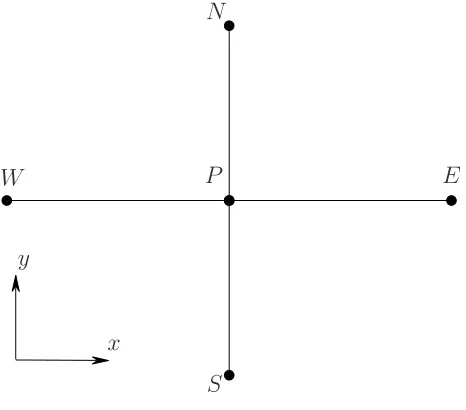
4.1 A grid point P and its neighbouring points on a Cartesian grid. 101

4.2 Square cavity flow, Re= 1000, 51_×51: convergence behaviour. IRBFE-ADI method using a time step of 6 _× 10−5 _converges

faster than the CD-ADI method using a time step of 3_×10−5_.

It is noted that the latter diverges for time steps greater than 3_×10−5_. _CM _{denotes the relative norm of the difference of the}

streamfunction fields between two successive time levels. . . 110

4.3 Square cavity flow, Re = 3200, 91_×91, solution at Re = 1000 used as initial guess: convergence behaviour. IRBFE-ADI method using a time step of 7_×10−6 _{converges faster than the CD-ADI}

method using a time step of 2_×10−6_{. It is noted that the}

lat-ter diverges for time steps grealat-ter than 2_×10−6_. _CM _denotes

the relative norm of the difference of the streamfunction fields between two successive time levels. . . 111

4.4 Square cavity flow, Re= 7500, 131_×131, solution atRe= 5000 used as initial guess: convergence behaviour. CD-ADI method uses a time step of 5_×10−7 _{and IRBFE-ADI method uses a time}

step of 1_×10−6_. _CM _{denotes the relative norm of the difference}

(29)

List of Figures xxviii

4.5 Square cavity flow, Re= 100, grid = 11_×11: streamlines. The contour values for CD-ADI and IRBFE-ADI plots are the same. 116

4.6 Square cavity flow, Re = 1000, grid = 51_×51: stream and iso-vorticity lines. The contour values are taken to be the same as those in Ghia et al. (1982) and Sahin and Owens (2003) respec-tively. Note the oscillatory behaviour near the top right corner in the case of CD-ADI method. . . 116

4.7 Square cavity flow, Re = 3200, grid = 91_×91: stream and iso-vorticity lines. The contour values are taken to be the same as those in Ghia et al. (1982) and Sahin and Owens (2003) respec-tively. Note the oscillatory behaviour near the top right corner in the case of CD-ADI method. . . 117

4.8 Square cavity flow,Re= 5000, grid = 111_×111: stream and iso-vorticity lines. The contour values are taken to be the same as those in Ghia et al. (1982) and Sahin and Owens (2003) respec-tively. Note the oscillatory behaviour near the top right corner in the case of CD-ADI method. . . 118

4.9 Square cavity flow, IRBFE-ADI, Re = 7500, grid = 131_×131: stream and iso-vorticity lines. The contour values are taken to be the same as those in Ghia et al. (1982) and Sahin and Owens (2003) respectively. . . 118

(30)

List of Figures xxix

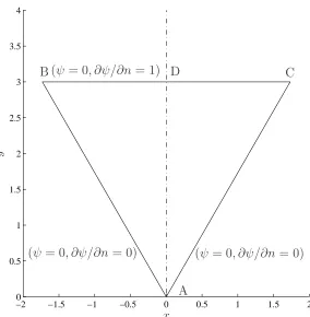
4.11 Triangular cavity flow: schematic outline of the computational domain and boundary conditions. Note that the characteristic length is chosen to be AD/3 to facilitate comparison with other published results (Ribbens et al. 1994, Kohno and Bathe 2006). 121

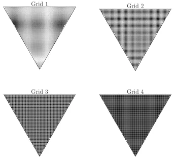
4.12 Triangular cavity flow: the computational domain is discretised by four Cartesian grids. . . 122

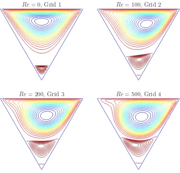
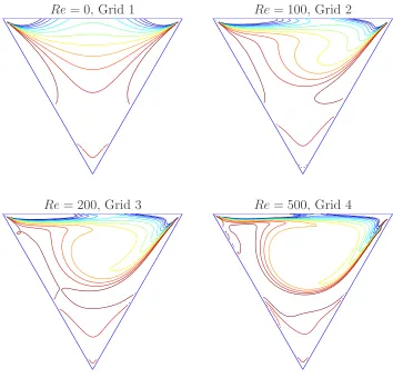
4.13 Triangular cavity flow: streamlines which are drawn using 21 equi-spaced levels between the minimum and zero values, and 11 equi-spaced levels between the zero and maximum values. . . 123

4.14 Triangular cavity flow: iso-vorticity lines which are drawn at intervals of ∆ω = 0.5 for a range of ₋5_≤ω_≤0.5. . . 124

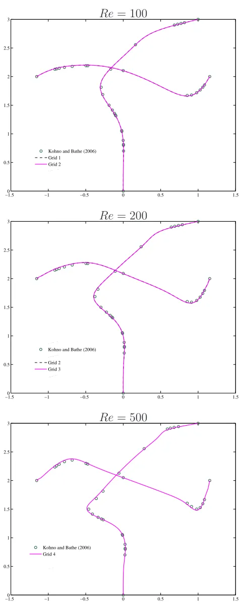
4.15 Triangular cavity flow: velocity profiles by the present method and the flow condition-based interpolation FEM (Kohno and Bathe 2006). . . 127

5.1 Schematic outline of a three-point stencil. . . 133

5.2 Schematic outline of a five-point stencil. . . 139

5.3 One-dimensional problem, Dirichlet boundary conditions only, ∆t = 0.001: Relative L2 errors of the approximation solution φ

att= 1 against the RBF width (β) for three different grids. . . 149

(31)

List of Figures xxx

5.5 One-dimensional problem, Dirichlet boundary conditions only, N = 63, ∆t = 0.001: Comparison of the accuracy of the first derivative at each time level between the classical Crank-Nicolson method and the present Crank-Nicolson method. For the latter, three values of β, i.e. 210,231 and 243, are employed. . . 150

5.6 One-dimensional problem, Dirichlet boundary conditions only, N = 11, β = 15, ∆t = 0.001: Error distribution on the problem domain of the present method and the direct IRBFE method (An-Vo et al. 2011b, 2013) for the first derivative att= 1. . . . 150

5.7 One-dimensional problem, Dirichlet and Neumann boundary con-ditions, N = 63, ∆t = 0.001: Comparison of the accuracy of the field variable at each time level between the classical Crank-Nicolson method and the present Crank-Crank-Nicolson method. For the latter, three values of β, i.e. 210,231 and 243, are employed. 152

5.8 One-dimensional problem, Dirichlet and Neumann boundary con-ditions,N = 63, ∆t = 0.001: Comparison of the accuracy of the first derivative at each time level between the classical Crank-Nicolson method and the present Crank-Crank-Nicolson method. For the latter, three values of β, i.e. 210,231 and 243, are employed. 153

5.9 Rectangular domain problem, Dirichlet boundary conditions only, Nx×Ny = 22×22, ∆t = 0.001: Relative L2 errors of the

ap-proximate solution φ at t= 0.6 against the RBF width (β). . . . 156

5.10 Rectangular domain problem, Dirichlet boundary conditions only, Nx×Ny = 22×22, ∆t = 0.001: Comparison of the accuracy of

(32)

List of Figures xxxi

5.11 Rectangular domain problem, Dirichlet boundary conditions only, Nx×Ny = 22×22, ∆t = 0.001: Comparison of the accuracy of

the first derivatives at each time level between the classical ADI method and the present ADI method. For the latter, three values of β, i.e. 170,180 and 190, are employed. . . 157

5.12 Rectangular domain problem, Dirichlet and Neumann boundary conditions, Nx × Ny = 22 ×22, ∆t = 0.001: Comparison of

the accuracy of the field variable at each time level between the classical ADI method and the present ADI method. For the latter, three values of β, i.e. 170,180 and 190, are employed. . . 157

5.13 Rectangular domain problem, Dirichlet and Neumann boundary conditions, Nx × Ny = 22 ×22, ∆t = 0.001: Comparison of

the accuracy of the first derivatives at each time level between the classical ADI method and the present ADI method. For the latter, three values of β, i.e. 170,180 and 190, are employed. . . 158

5.14 Circular domain problem: Geometry and discretisation. Bound-ary nodes denoted by _◦ are generated by the intersection of the grid lines and the boundary. . . 159

5.15 Circular domain problem: Exact solution over an extended domain.160

5.16 Circular domain problem, ∆t = 0.001, β = 330: The accuracy at each time level by the present ADI method using three grids. 162

5.17 Circular domain problem, Nx ×Ny = 141×141, ∆t = 0.001,

(33)

List of Figures xxxii

5.18 Lid-driven cavity flow, Re = 1000, grid = 61_×61, solution at Re= 400 used as initial guess: Convergence behaviour. Present method using a time step of 1_×10−4 _{converges faster than the}

IRBFE-ADI method using a time step of 5_×10−5_{and the explicit}

treatment of convection method (ETCM) using a time step of 1_×10−5_{. It is noted that the IRBFE-ADI and the ETCM diverge}

for the time steps greater than 5_×10−5 _{and 1}_×₁₀−5 _{respectively.170}

5.19 Lid-driven cavity flow, Re = 3200, grid = 91_×91, solution at Re= 1000 used as initial guess: Convergence behaviour. Present method using a time step of 1_×10−5 _{converges faster than the}

explicit treatment of convection method (ETCM) using a time step of 1_×10−6_{. It is noted that the ETCM diverges for the time}

steps greater than 1_×10−6_{. . . 171}

5.20 Lid-driven cavity flow, Re = 1000, grid = 71 _× 71: velocity profiles along the vertical and horizontal centrelines. [*] is Botella and Peyret (1998). . . 173

5.21 Lid-driven cavity flow: contour plots of streamfunction (left) and vorticity (right) for several values of Re. The iso-vorticity lines are taken as 0,_±0.5,_±1,_±2,_±3,_±4,_±5. . . 174

5.22 Lid-driven cavity flow, Re= 3200, grid= 91_×91: overall stream lines (upper figures) and a magnified view of those in the upper right corner. The contour values for CD-ADI method and the present method plots are the same. . . 175

(34)

List of Figures xxxiii

5.24 Lid-driven cavity flow: stream and iso-vorticity lines by the present method for Re = 5000 and Re = 7500. The iso-vorticity lines are taken as 0,_±0.5,_±1,_±2,_±3,_±4,_±5. . . 177

6.1 A computational domain Ω with the coarse grid (black dashed lines) and dual coarse grid (black solid lines); dashed and solid red lines indicate a selected control volume Ωk and a selected dual

coarse cell Ωel_{, respectively. Shown underneath is an enlarged}

control volume, on which is imposed a n_×n = 11_×11 local fine grid. It can be seen that the size of global fine grid (dashed green lines) is 41_×41. . . 187

6.2 Local indices of dual cells and nodal points associated with a coarse grid node xk and xk≡x1. . . 189

6.3 A CV discretisation scheme in 1D: node iand its associated con-trol volume. The circles represent the nodes, and the vertical dash lines represent the faces of the control volume. . . 194

6.4 Schematic outline for a 2D control volume on the fine scale grid. 203

6.5 One-dimensional example 1, ε = 0.01, N = 11, n = 101: basis functions (a) and correction function (b) associated with the first coarse cell (l = 1). It is noted that the coarse cell is mapped to a unit length. . . 212

6.6 One-dimensional example 1: mesh convergence of a basis function.214

(35)

List of Figures xxxiv

6.8 One-dimensional example 1, ε = 0.01, N = 11,n = 101: second derivatives obtained by the present method in comparison with that obtained by the exact solution. . . 219

6.9 One-dimensional example 2, ε = 0.01, N = 51, n = 101: field variable, its first and second derivatives obtained by the present method in comparison with the exact solution. . . 223

6.10 Two-dimensional example 1: collection of all correction functions on the problem domain obtained with a grid system of N_×N = 5_×5, n_×n = 21_×21. . . 225

6.11 Two-dimensional example 1, N _×N = 5_×5, n_×n = 81_×81 (left) andN_×N = 33_×33, n_×n = 11_×11 (right): effect of the number of smoothing steps ns on the convergence behaviour. . . 226

6.12 Two-dimensional example 2: typical basis and correction func-tions for the cases of ε = 0.1 using a grid system of N _×N = 5_× 5, n _× n = 21_× 21 and ε = 0.01 using a grid system of N_×N = 11_×11, n_×n = 21_×21. . . 229

6.13 Two-dimensional example 2: contour plots of correction func-tions on the problem domain for the cases ofε= 0.1 using a grid system ofN _×N = 5_×5, n_×n = 21_×21 and ε= 0.01 using a grid system ofN _×N = 11_×11, n_×n= 21_×21. . . 230

6.14 Two-dimensional example 2, ε = 0.1, N _×N = 5_×5, n_×n = 61_×61 (left) andN_×N = 25_×25, n_×n= 11_×11 (right): effect of the number of smoothing stepsns on the convergence behaviour.234

(36)

List of Figures xxxv

6.16 Two-dimensional example 2, ε= 0.1,ns = 1: convergence of the

present method and the fine scale solver with increasing sizes of the global fine grid; grid 1 = 241_×241 (N_×N = 5_×5, n_×n= 61_×61), grid 2 = 281_×281 (N _×N = 5_×5, n_×n= 71_×71), grid 3 = 321_×321 (N _×N = 5_×5, n_×n = 81_×81). . . 238

(37)

Chapter 1

Introduction

This chapter starts with the motivation for the present research. Then model problems are defined, followed by a review and discussion on multiscale meth-ods. A brief review of radial basis function serve to introduce new ideas and objectives of the present research. Finally, the outline of the dissertation is described.

1.1

Motivation

(38)

prac-1.2 Problem definition 2

tical problems, because of overwhelming costs, a direct representation of the full fine-scale solution is simply impossible on today’s computer resources. This research project is concerned with the development of a high-order computa-tional procedure which is capable of solving multiscale elliptic equations arising from the modelling of multiphase materials on the present computing facilities. The proposed procedure makes use of several recent advances in computational mechanics, including the non-polynomial multiscale space approach (heteroge-nous media) and spectral universal interpolants based on integrated radial basis functions (high-order approximations).

1.2

Problem definition

The prediction of deformation or thermal behaviour of composites presents sig-nificant challenges. One must take into consideration the behaviour of individual constituents (i.e. reinforcements particles, fibres, whiskers and platelets -and resin/matrix), the interaction between these components -and the involve-ment of multiple length scales and also possibly multiphysics. Fortunately, certain phenomena/problems can be modeled by multiscale elliptic equations. To capture the solution at a fine scale, the use of traditional direct approaches, e.g. multigrid methods, domain decomposition methods and adaptive mesh re-finement techniques, leads to discrete systems that have very large degrees of freedom from both spatial and temporal discretisations. For a brief illustration, we consider the following elliptic equation which arises from the modelling of composite materials and subsurface flows

−∇ ·(aǫ(x)_∇u) =f(x) in Ω, (1.1)

where aǫ₍_x_{) is the material property tensor involving a small scale parameter}

(39)

1.3 Review of multiscale methods 3

to (1.1) gives an overly pessimistic estimate of error O(h/ǫ) in the H1 _norm,

where h is the mesh size. Direct methods clearly cannot converge when h > ǫ and it thus requires a mesh size to be much smaller than the small length scale (h _≪ ǫ). It can be seen that tremendous amounts of computer memory and CPU time required by these methods can easily exceed the limit of today’s computing resources. Consequently, several classes of numerical methods have been developed to deal with the multiscale nature of the solution. Examples include homogenisation methods (Kalamkarov et al. 2009), heterogeneous mul-tiscale methods (E and Engquist 2003b) and mulmul-tiscale shape function methods (Hou and Wu 1997). These methods seek to capture the fine scale effect on the coarse scales via a multi-stage resolution of the fine scale features. As a result, they make the solution of a multiscale problem possible, from which the coarse scale/bulk properties of multiphase materials such as the effective conductivity, elastic moduli and permeability can be predicted. However, dense meshes are still typically required in commonly employed low order approximations.

1.3

Review of multiscale methods

Consider the model problem (1.1). We assume that (i) the tensora(y),y=x/ǫ, is smooth and periodic in the domain of the variable y, namely Y, and (ii) boundary conditions for u are homogeneous on the whole boundary, i.e. u= 0 on∂Ω. We use_h†i=R_Y _†dy/_|Y_|to denote the volume average of the physical quantity _† over Y.

(40)

large system associated with the fine mesh resolution in order to achieve

cost of multiscale method

cost of direct method ≪1. (1.2)

For HMM and MFEM, fine-scale information is derived from the solution of the following auxiliary fine scale problem

−∇ ·(aǫ₍_x₎_∇_φ(_x_{)) = 0 in} _D_⊂_Ω, _(1.3)

where D represents a local domain that is named a unit cell for HMM or an element for MFEM, and φ(x)s are local adaptive functions used to calculate coarse element stiffness matrices for HMM and shape functions for MFEM.

For MHM, fine-scale information is derived from the following cell problem

∇y·(a(y)∇yχj(y)) =

∂aij(y)

∂yi

, (1.4)

where χj(y)s, which are named influence functions, are chosen to be periodic

with zero mean, i.e. _hχji= 0.

1.3.1

Mathematical homogenisation method

The mathematical homogenisation method (MHM) has been traditionally used as a primary tool for analysing heterogeneous medium and its details were explained in, for example, Babuˇska (1976), Benssousan et al. (1978), Oleinik et al. (1992), Guedes and Kikuchi (1990), Hassani and Hinton (1998), Takano et al. (2000), Fish and Yuan (2005). Based on the assumptions of microstructure periodicity and uniformity of a unit cell domain, the homogenisation theory decomposes the boundary value problem into a unit cell (fine scale) problem and a global (coarse scale) problem.

(41)

con-1.3 Review of multiscale methods 5

stituents are linearly elastic. In the following, for brevity, we present MHM for one component of the displacement vector. The actual displacement com-ponent, denoted by uǫ_{, may be periodically oscillating due to the fine scale}

heterogeneity. The homogenised model can provide the homogenised displace-ment, denoted by u0. The differences between the actual displacement uǫ and

the homogenised displacement u0 are determined as the perturbed

displace-ment, denoted byu1, multiplied by the small parameter ǫ, and so on. Then, a

double-scale asymptotic expansion of the actual displacement is

uǫ(x) =u0(x) +ǫu1(x,y) +ǫ2u2(x,y) +· · · , (1.5)

where ui(x,y), i = (1,2, . . .), are functions of both scales and y-periodic in

Y. The actual displacement uǫ _{is also a function of both scales, whereas the}

homogenised displacement u0 is only a function of the coarse scale. The latter

is the solution of the homogenised equation

−∇ ·a⋆_∇u0 = f in Ω, (1.6)

u0 = 0 on ∂Ω, (1.7)

wherea⋆ _{is the effective material coefficient tensor, given by}

a⋆_ij =

aik(y)

δkj−

∂χj

∂yk

. (1.8)

It was proved in Benssousan et al. (1978) thata⋆_{is symmetric and positive}

defi-nite. The leading perturbed displacementu1 in equation (1.5) can be expressed

in terms of the homogenised displacement u0 as

u1(x,y) = −χj

∂u0

∂xj

, (1.9)

(42)

equation (1.4), are also refereed to as the characteristic displacements (Takano et al. 2000). The proof of the existence and uniqueness of the solution of equa-tion (1.4) in weak-form sense and the validity of equaequa-tion (1.9) were detailed in several works (Babuˇska 1976, Benssousan et al. 1978, Oleinik et al. 1992, Guedes and Kikuchi 1990, Hassani and Hinton 1998). Since there is no assumption on the geometrical configuration of the constituents, the homogenisation theory can tackle arbitrary complex microstructures. The fine scale stress tensorσij is

given in Xing et al. (2010). The coarse scale stresses are defined as the volume average of the fine scale stresses within a unit cell

σH_ij =_hσiji. (1.10)

A salient feature of MHM is that the fine scale solution is completely described on the coarse scale, see equations (1.9). Nevertheless, the influence functions are computed at a material point from equation (1.4) prior to the fine scale solution.

It is apparent that meshes of a unit cell need to be fine enough for accu-rately computing derivatives of the influence functions and homogenised dis-placements. Moreover, the second order perturbationu2(x,y) in equation (1.5)

may be required when the constituents have highly contrast properties. The error source also comes from the boundary condition since in generalu1 6= 0 on

∂Ω. Therefore, the boundary condition u_|∂Ω = 0 should be enforced through

the first-order corrector termθǫ (Benssousan et al. 1978), which is given by

∇ ·(aǫ(x/ǫ)_∇θǫ) = 0 in Ω, (1.11)

θǫ = u1(x,x/ǫ) on ∂Ω. (1.12)

(43)

classical homogenisation theory. Recently, Kalamkarov et al. (2009) reviewed the state-of-the-art of asymptotic homogenisation techniques in the analysis of composite materials and thin-walled composite structures.

The implementation of MHM consists of three steps as follows.

• Solving the influence functions from equation (1.4) through FEM and evaluating the homogenised (effective) material properties from equation (1.8);

• Solving the homogenised displacement from equations; (1.6)-(1.7) with the effective material properties through FEM;

• Post-processing on the micro and macro levels.

1.3.2

Heterogeneous multiscale method

The heterogeneous multiscale method (HMM) (E and Engquist 2003b, 2005; Ming and Yue 2006; Ming and Zhang 2007; E and Engquist 2003a; Abdulle 2007; E et al. 2007) can be viewed as a general method for the computation of multiscale problems. HMM involves two main calculations. The first one is to select an overall macroscopic scheme such as FEM for the coarse scale variables on a coarse mesh, and the second one is employed to estimate the missing coarse scale data by solving locally the fine scale problem. To solve for the coarse scale features of the problem (1.1), one can employ the strain energy U of the global structure, which generally has the following form

U = 1 2

Z

Ω

(44)

Assuming that the strain energy is calculated by means of the numerical quadra-ture rule as

U = 1 2

X

D∈H

|D_| X

xl∈D

αla⋆(xl)(∇u0(xl))2, (1.14)

where H is the coarse mesh, xl and αl are respectively the quadrature points

and the weights in element D, and a⋆₍_x

l) is the effective material coefficient

at those quadrature points and calculated by (1.8). Expression (1.14) must be approximated by solving the problem in the small domain Iδ(xl) near the

quadrature point xl, which is governed by

∇ ·(aǫ(x)_∇v(x))) = 0, x_∈Iδ(xl), (1.15)

whereIδ(xl) is a square of size δ centered at xl. Different boundary conditions

on ∂Iδ(xl) and their effects were discussed in Yue and E (2007). Equation

(1.15) can be typically solved by FEM in just several small domains of a unit cell rather than solving a whole cell problem. Then equation (1.14) is evaluated in the following way

U = 1 2

X

D∈H

|D_| X

xl∈D αl

Z

Iδ(xl) a⋆₍_x

l)

δ2 (∇v(xl))

2_dI. _(1.16)

Finally, the HMM solution u0(x) is obtained by solving

minX

D∈H

U ₋

Z

D

f(x)u0(x)dD

, (1.17)

which can be understood as the weak form of equation (1.1). It is noteworthy that the cost of HMM depends on the size of δ. HMM can take advantages of the possible scale separation in the problem, but becomes similar to the fine scale solvers when there is a lack of scale separation.

All demonstrations of HMM assume that a⋆₍_x_{) are smooth, symmetric and}

(45)

How-1.3 Review of multiscale methods 9

ever, this assumption cannot be applicable for multiphase materials. If there are two or more kinds of materials in Iδ(xl), the accuracy will be deteriorated

when solving equation (1.15) with the homogenised boundary conditions which cannot model the material jumps on the boundaries of Iδ(xl). Therefore, the

application of HMM in composite structures needs to be studied in depth.

It is well known that the microstructure information in uǫ _{is used for the local}

stress analysis. This information can be recovered using a simple postprocessing technique based on u0 (E and Engquist 2003a, Oden and Vemaganti 2000).

Assume that we are interested in recovering uǫ _and _∇_uǫ _{only in a local domain}

or a unit cellD. One of the recovering approaches is the local model refinement (Oden and Vemaganti 2000), in which the following auxiliary problem,

−∇ ·(aǫ(x)_∇u(x)) =f(x) in D_⊂Ω, (1.18) u(x) =u0(x) on ∂D,

is solved, and the approximationuǫ_{with micro information, whose error is finite,}

is then obtained (E and Engquist 2005). Another recovering approach is similar to the asymptotic expansion as in MHM. Define the first order approximation of uǫ₍_x_{) as}

uǫ(x) =u0(x) +ǫχj

∂u0

∂xj

, (1.19)

where the influence function χj is the solution of equation (1.4).

HMM generally gives a framework that allows us to maximally take advantage of the special features of the problem such as scale separation; for problems without any special features, HMM becomes a fine scale solver. The savings in HMM, compared with the cost of solving the full fine scale problem, comes from the fact that Iδ(xl) can be chosen to be smaller than D, and the small

domain Iδ(xl) is determined by many factors, including the accuracy and cost

(46)

HMM has been applied to a large variety of homogenisation problems either linear or nonlinear, periodic or non-periodic, stationary or dynamic (E and En-gquist 2006), and can be naturally extended to higher order by using higher order finite elements as the macroscopic solver. Recently, E et al. (2007) pre-sented a state-of-the-art review of HMM, including the fundamental philosophy, and the main process for complex fluids, micro-fluidics, solids, interface prob-lems, stochastic problems and statistically self-similar problems. Chen (2009) has incorporated various macroscopic solvers, including finite differences, finite elements, discontinuous Galerkin, mixed finite elements, control volume finite elements, and nonconforming finite elements, into HMM and pointed out their advantages, shortcomings and adaptabilities.

The computational sequence of HMM includes four steps:

• Solving the sub-local problems governed by equation (1.15) around the quadrature points of a coarse element to capture the effects of microstruc-ture;

• Evaluating the strain energy through equation (1.16);

• Solving the homogenised displacementu0from equation (1.17) using FEM;

• Recovering the micro information inuǫ_{by solving equation (1.18) or using}

equation (1.19).

1.3.3

Multiscale finite element method

(47)

element shape functions reflecting the local property of the differential opera-tor. The MFEM is applicable to general multiscale problems without restrictive assumptions, and the construction of the shape functions for a coarse scale ele-ment is independent from each other.

In contrast with some empirical numerical upscaling methods (Sangalli 2003), MFEM is systematic and self-consistent. The idea of constructing finite element shape functions based on local differential operator in MFEM is an extension of the work of Babuˇska and Osborn (1983), which incorporates the fine scale information into the basis functions by solving the original fine scale differential equations on each element with proper boundary conditions.

The over-sampling MFEM reduces the effect of the boundary layers occurring at the inter-element boundaries by an indirect approach in constructing the base functions. Instead of directly working on an elementD, a domain S larger than D is used with diam(S) =H > h+ǫ. Any reasonable boundary condition can be imposed on the boundary of domain S in solving equation (1.3) to obtain temporary base functions denoted as ψi with i = (1, . . . , d) in which d is the

number of element nodes. One then constructs the actual base functions from the linear combination of ψjs

φi = d

X

j=1

cijψj, i= (1, . . . , d), (1.20)

wherecij are the constants determined by the conditionφi(xj) =δij.

(48)

1.4 Discussion 12

the over-sampling MFEM are as follows.

• Solving equation (1.3) on a domain S for the auxiliary shape functions ψj;

• Evaluating the over-sampling multiscale finite element shape functionsφis

over a coarse element using equation (1.20);

• Solving the coarse mesh problem by using FEM.

1.4

Discussion

A brief review on multiscale computational methods (MHM, HMM, MFEM) for multiphase materials in Section 1.3 provides an understanding of their phi-losophy and main features. As discussed, MHM is based on the homogenisation theory and hence its range of applications is usually limited by restrictive as-sumptions on the media, such as scale separation and periodicity (Benssousan et al. 1978). It is also expensive to be used for solving problems with many sep-arate scales since the cost of computation grows exponentially with the number of scales (Hou and Wu 1997). HMM is more general and can be applied to prob-lems with random coefficients. However, its effectiveness is strongly dependent on the material structure assumptions such as scale separation. Without this assumption, HMM is equivalent to a direct solver. In the last case, MFEM is applicable to general multiple-scale problems without restrictive assumptions. In contrast to MHM, the number of scales are irrelevant to the computational cost in MFEM (Hou and Wu 1997). MFEM is systematic and self-consistent, which makes it easier to analyse especially large scale problems. Nevertheless, the accuracy of MFEM is low in the order of O(ǫ/h) (Hou and Wu 1997) and its convergence for continuous scale problems needs to be further studied.

(49)

1.4 Discussion 13

is the error source coming from the cell problem (MHM, HMM) or element problem (MFEM). It was pointed out by Babuˇska and Osborn (1983) in the FEM context and recently by Yuan and Shu (2008) and Wang et al. (2011) in the context of discontinuous Galerkin method (DGM) that an approximation space Sr _{should be constructed as}

Sr=_{φ:_{∇ ·}(aǫ(x)_∇φ)_|I ∈Pr−2(I)} for r = 1,2,· · ·, (1.21)

whereI denotes the cell or element in the spatial discretisation, Pr_{(I) denotes}

the space of polynomials of degree less than or equal toronIandP−1_(I_{) =}_{₀_}_.

It can be seen that the approximation spaces of current multiscale methods in the literature correspond to S1 _{except for the DGM case (e.g. Yuan and Shu}

2008, Wang et al. 2011), in which high convergence rates are obtained forr >1.

Generally, conventional numerical methods such as finite element methods (FEMs), finite difference methods (FDMs) and finite volume methods (FVMs) are utilised to numerically solve both the fine scale and coarse scale problems in a theoretical framework (MHM, HMM, MFEM). These methods are typically of low order of accuracy and provide aC0 _{solution. It is noted that there are high-order}

formu-lations, those using Hermite interpolation for instance, e.g. (Zienkiewicz 1971, Watkins 1976, Holdeman 2009) for FEM and e.g. (Qiu and Shu 2003, 2005) for FVM, that can afford higher continuity. To the best of our knowledge, such high-order methods currently are not yet applied to multiscale model problems of interest in this thesis. The field variables and their derivatives are highly oscillating in multiscale problems, posing a great challenge for conventional low-order methods.

A 1D example below, having an exact solution, can clearly display this challenge

−_dxd

aǫ(x)du dx

(50)

1.4 Discussion 14

0 0.1 0.2 0.3 0.4 0.5 0.6 0.7 0.8 0.9 1 0 0.02 0.04 0.06 0.08 0.1 0.12 0.14 0.16 0.18 x u ( x ) (a)

0.14 0.16 0.18 0.2 0.22 0.24 0.26 0.064 0.066 0.068 0.07 0.072 0.074 0.076 0.078 0.08 0.082 0.084 x u ( x ) (b)

0 0.1 0.2 0.3 0.4 0.5 0.6 0.7 0.8 0.9 1 −1.4 −1.2 −1 −0.8 −0.6 −0.4 −0.2 0 0.2 0.4 0.6 x d u d x (c)

[image:50.595.116.512.112.498.2]

0 0.1 0.2 0.3 0.4 0.5 0.6 0.7 0.8 0.9 1 −250 −200 −150 −100 −50 0 50 100 150 200 x d 2u d x 2 (d)

Figure 1.1: Exact solution of problem (1.22)-(1.24) for ǫ = 0.01: (a) field variable, (b) its zoomed part, (c) its first-order derivative, (d) its second-order derivative.

with boundary conditions

u(0) =u(1) = 0 (1.23)

where

aǫ(x) = 1

2 +x+ sin(2πx/ǫ). (1.24)

(51)

1.5 Radial basis functions (RBFs) 15

important issues in solving problem (1.1) is to recover the details of_∇uǫ

(first-order derivative) since they contain information of great practical interest, such as the stress distribution and heat flux in composite materials or the velocity field in a porous medium (Ming and Yue 2006). In addition, even in the theoreti-cal framework such as MHM, accurate approximations of derivatives of influence functions are necessary for evaluating the homogenised material coefficient in equation (1.8) and coarse scale displacement u0 in equations (1.6)-(1.7). It is

also noteworthy that the first perturbation displacement u1 is also estimated

from the first-order derivative of u0 in equation (1.9). In the case of MFEM, if

the basis functionsφs are obtained by a conventional linear FEM, they are only C0 _{functions, causing significant error in first-order derivative approximation}

and, as a result, it is impossible to approximate second-order derivatives. The discontinuity of derivatives is usually mitigated by using fine meshes, which can make conventional methods inefficient or even impracticable. Therefore, it is desirable to develop a method that has a higher order continuity of the solution across elements and also has a higher level of accuracy and efficiency. Incorporation of radial basis functions into the discretisation frameworks as trial functions can be a potential way to achieve these objectives.

1.5

Radial basis functions (RBFs)

(52)

1.5 Radial basis functions (RBFs) 16

with the point-collocation formulation, the resultant discretisation methods are truly meshless (e.g. Kansa (1990)). RBF-based collocation methods can be applied to differential problems defined on irregular domains without added difficulties. Apart from point-collocation, RBFs have also been employed as trial functions in other formulations such as the Galerkin, subregion collocation and inverse statements, resulting in enhanced rates of convergence (error of O(hα₎

with α > 2) of these approaches. Works in this research trend include Atluri et al. (2004), Sellountos and Sequeira (2008), Orsini et al. (2008), Mohammadi (2008).

In a conventional RBF scheme (Kansa 1990), the original function is decom-posed into RBFs and its derivatives are then obtained through differentiation. Some RBF schemes such as those based on multiquadric (MQ) function are known to possess spectral accuracy with error in the O(λχ_{), where 0} _{< λ <}_1.

Through numerical experiment, for a certain range of the RBF-widtha, Cheng et al. (2003) established the error estimate asO(λ√a/h_{). In the approximation}

of kth derivative, Madych (1992) showed that the convergence rate is reduced toO(λχ−k_{). To avoid such reduction of convergence rate caused by}

(53)

1.6 Objectives of the present research 17

et al. 2009, Ho-Minh et al. 2009).

Although 1D-IRBF schemes can yield a high level of accuracy using a relatively coarse grid, their system matrices are not as sparse as those produced by con-ventional FDMs. In addition, for a stable calculation, these schemes are limited to small values of the RBF width.

1.6

Objectives of the present research

In this research project, we further localise the 1D-IRBFs to construct a new type of element for the discretisation of ODEs/PDEs in point/subregion col-location formulations on Cartesian grids. The proposed element involves two nodes, called 2-node IRBFE, wherein the 1D-IRBFs are implemented with two RBF centres only and the approximations are nonoverlapping. It can be seen that the use of two RBFs (a smallest RBF set) allows a wide range of the RBF width to be used and leads to very sparse system matrices. Moreover, the approximate solution is guaranteed to be C2_{-continuous across the}

inter-face of IRBFEs. We then verify the novel formulations through the solution of benchmark nonlinear flows of an incompressible Newtonian fluid (e.g. flows in lid-driven cavities and flows past a circular cylinder in a channel). We optimise the efficiency of the present approaches with the alternating direction implicit (ADI) procedure (Peaceman and Rachford 1955, Douglas and Gunn 1964) via different strategies. Finally, we introduce these proposed IRBFEs and subre-gion collocation into the non-polynomial multiscale space framework for solving the multiscale elliptic problems.

Accuracy will be enhanced by the following key features.

(54)

1.7 Outline of the Dissertation 18

• Integration rather than differentiation is employed to construct the RBF approximations.

• The computed solution is aC2 _{function rather than the usual} _C0_.

Efficiency will be enhanced by the following key features.

• The IRBFE involves only two RBF centres, leading to a sparse system matrix.

• Cartesian grids are used to represent the problem domain. It is clear that generating a Cartesian grid is much simpler and easier than generating a finite-element mesh. Moreover, ADI procedure (Peaceman and Rach-ford 1955, Douglas and Gunn 1964) can be straightforwardly applied to accelerate computational processes.

• Point collocation formulation and control volume formulation employed with the middle point rule are utilised to discretise the governing equation. These discretisation approaches are integration free.

• Meaningful solutions can be obtained on a relatively coarse grid as mass and momentum conservations are preserved over control volumes associ-ated with the grid nodes.

The central goal of the present research is to obtain multiscale solutions accu-rately and effectively.

1.7

Outline of the Dissertation

(55)

• Chapter 2 presents a new C2_{-continuous control volume discretisation}

method, based on Cartesian grids and 2-node IRBFEs, for the solution of second-order elliptic problems in one and two dimensions. The proposed 2-node IRBFEs are then utilised by the following chapters.

• Chapter 3 develops 2-node IRBFEs for the simulation of incompressible viscous flows in two dimensions. Emphasis is placed on (i) the incorpo-ration of C2_{-continuous 2-node IRBFEs into the subregion and point}

col-location frameworks for the discretisation of the streamfunction-vorticity formulation on Cartesian grids; and (ii) the development of high order upwind schemes based on 2-node IRBFEs for the case of convection-dominant flows.

• Chapter 4 presents a C2_{-continuous alternating direction implicit (ADI)}

method based on 2-node IRBFEs for the solution of the streamfunction-vorticity equations governing steady 2D incompressible viscous fluid flows. Unlike in Chapters 2 & 3 the solution strategy in this chapter consists of multiple use of a one-dimensional sparse matrix (associated with grid lines) algorithm that helps save the computational cost.

• Chapter 5 presents a novel C2_{-continuous compact scheme based on}

2-node IRBFEs. The proposed C2_{-continuous compact scheme is applied}

to the discretisation of second-order parabolic equations in one- (1D) and two-space dimensions (2D) in an implicit manner. As in Chapter 4 the ADI procedure (Peaceman and Rachford 1955, Douglas and Gunn 1964) is applied for the time integration in 2D. However, the one-dimensional matrices associated with grid lines are optimised to be in standard tridi-agonal form which can be solved efficiently by the Thomas algorithm. Moreover, the typical matrix size is half of that obtained in Chapter 4 and equal to the number of nodal unknowns of the dependent variable only.

(56)

multiscale basis function approach and IRBFEs, for the solution of mul-tiscale elliptic problems with reduced computational cost. Unlike other methods based on multiscale basis function approach, sets of basis and correction functions here are obtained throughC2_{-continuous IRBFE-CV}

formulation.

(57)

Chapter 2

Two-node IRBF elements and a

C

2

-continuous control-volume

technique

This chapter presents a new control-volume discretisation method, based on Cartesian grids and integrated-radial-basis-function elements (IRBFEs), for the solution of second-order elliptic problems in one and two dimensions. The gov-erning equation is discretised by means of the control-volume formulation and the division of the problem domain into non-overlapping control volumes is based on a Cartesian grid. Salient features of the present method include (i) an element is defined by two adjacent nodes on a grid line, (ii) the IRBF ap-proximations on each element are constructed using only two RBF centres (a smallest RBF set) associated with the two nodes of the element and (iii) the IRBFE solution is C2_{-continuous across the interface between two adjacent}

(58)

2.1 Introduction 22

element-based solutions, allowing a better estimate for the physical quantities involving derivatives. Numerical results indicate that (i) the proposed method can work with a wide range of the shape-parameter/RBF-width and (ii) the proposed technique yields more accurate results and faster convergence, espe-cially for the approximation of derivatives, than the standard control-volume technique.

2.1

Introduction

Traditional techniques used for solving second-order elliptic differential equa-tions include overlapping finite difference methods (FDMs), non-overlapping finite element methods (FEMs), boundary element methods (BEMs) and con-trol volume methods (CVMs). These methods typically utilise polynomials as an interpolator. To avoid notorious polynomial snaking phenomena, low-order polynomials such as linear variations are widely used, usually leading to errors of orderh2_{, where} _h_{is the mesh spacing. For element-based solutions, only the}

ap-proximating function (not its partial derivatives) is continuous across elements (i.e. C0 _{continuity). The overall error can be reduced by using progressively}

denser meshes. A mesh needs be sufficiently fine to mitigate the effects of discon-tinuity of partial derivatives. It is thus desirable to have discretisation methods that can produce a solution of higher-order continuity across elements. There are high-order formulations in the literature, for instance those using Hermite interpolation e.g. (Zienkiewicz 1971, Watkins 1976, Holdeman 2009) for FEM and e.g. (Qiu and Shu 2003, 2005) for FVM that can provide such high-order continuity. Here, we develop a high-order continuity method based on IRBF interpolation and control-volume formulation.