Partially Coherent Lab Based X ray Micro Computed Tomography

Micro Computed Tomography

Heyang Li (Thomas)

February 2017

A thesis submitted for the degree of Doctor of Philosophy of The Australian National University.

Research School of Physics and Engineering. Department of Applied Mathematics.

Supervisors: Dr. Andrew Kingston, Dr. Glenn Myers, and Dr. Adrian Sheppard

c

I express my deepest gratitude to my supervisors Dr. Andrew Kingston, Dr. Glenn Myers, Dr. Trond Varslot, and A/Prof. Adrian Sheppard who has put in a great deal of support at the start of my PhD research.

Dr. Kingston, Dr. Myers, and A/Prof. Sheppard involved in every topic of my PhD research. Their generous support, inspiration and insightful guid-ance have helped me through all the good and bad time of my research, and writing my thesis. They introduced me to many researchers in the field. They encouraged me to learn a diversity of skills and to expand my horizon as a postgraduate student at the Australian National University, and made my PhD research a really rewarding journey.

I would like to thank lab technicians Dr. Michael Turner and Dr. Levi Beeching for doing innovative and vital experiments with me. I show grat-itude to Dr. Shane Latham, a researcher and programmer for helping to fix bugs and issues in software code. I thank Dr. Benoit Recur, a postdoc for his input to my source deblurring work. Also thanks for the help received from members of department: Mr. Timothy Sawkins, Dr. Andy Christy, Prof. Vincent Craig, Prof. Denis Evans, Dr. Wilfred Fullagar, Mr. Carl Yang, and Ms. Martina Landsmann.

I thank fellow PhD candidates Mahsa Paziresh, Mr. Muidh Alheshibri and Rex Li for the mutual support and encouragement. I show my gratitude to the RSPE School of Computing Unit for fixing up my computer and general software issues. I thank the National Computational Infrastructure (NCI) for supercomputer access.

A special thanks goes to my parents Jenny and Simon for their emotional support and being amazing parents throughout my PhD study, and writing my thesis. They have put in extra efforts at home to ensure I could focus on writing my thesis. Also I thank Jenny for reading my thesis.

ematics for funding my conference attendance: ICTMS 2013 in Belgium, SPIE 2014 in USA, and ICTMS 2015 in Canada.

This thesis contains no material, which has been accepted for award of any other degree or diploma in any institu-tion. To the best of my knowledge, this thesis contains no material published or written by another person, except where due reference is made in the text.

Signed:

Heyang Li (Thomas)

X-ray micro computed tomography (CT) is a useful tool for imaging 3-D in-ternal structures. It has many applications in geophysics, biology and ma-terials science. Currently, micro-CT’s capability are limited due to validity of assumptions used in modelling the machines’ physical properties, such as penumbral blurring due to non-point source, and X-ray refraction. There-fore many CT research in algorithms and models are being carried out to overcome these limitations.

This thesis presents methods to improve image resolution and noise, and to enable material property estimation of the micro-CT machine developed and in use at the ANU CTLab. This thesis is divided into five chapters as outlined below.

The broad background topics of X-ray modelling and CT reconstruction are explored in Chapter 1, as required by later chapters. It describes each X-ray CT component, including the machines used at the ANU CTLab. The mathematical and statistical tools, and electromagnetic physical models are provided and used to characterise the scalar X-ray wave. This scalar wave equation is used to derive the projection operator through matter and free space, and basic reconstruction and phase retrieval algorithms. It quantifies the four types of X-ray interaction with matter for X-ray energy between 1 and 1000 keV, and presents common assumptions used for the modelling of lab based X-ray micro-CT.

in Chapter 3. For weakly attenuating samples, intensity variation due to phase contrast is a significant fraction of the total signal. If phase contrast is incorrectly modelled, the reconstruction would not correctly account the phase contrast, therefore it would contribute to undesirable artefacts in the reconstruction volume. Here I present a novel Linear Iterative multi-energy PR algorithm. It enables material property estimation for the near field sub-micron X-ray CT system and reduces the noise and artefacts. This PR algo-rithm expands the validity range in comparison to the single material and data constrained modelling methods. I have also extended this novel PR algorithm to assume a polychromatic incident spectrum for a non-weakly ab-sorbing object.

Chapter 4 outlines the space filling X-ray source trajectory and reconstruc-tion, on which I contributed in a minor capacity. This space filling trajec-tory reconstruction have improved the detector utilisation and reduced non-uniform resolution over the state-of-the-art 3-D Katsevich’s helical reconstruc-tion, this patented work was done in collaboration with FEI Company.

Acknowledgements . . . iii

Declaration . . . v

Abstract . . . vii

List of Acronyms . . . xvii

List of Symbols . . . xix

1. Introduction and Background . . . 1

1.1 Why X-rays? . . . 3

1.1.1 Development of X-ray Computed Tomography (CT) . . 4

1.2 X-ray Micro-CT System and Comparison . . . 4

1.2.1 X-ray Source . . . 5

1.2.2 Imaged Object . . . 9

1.2.3 Stage . . . 11

1.2.4 Detector . . . 12

1.2.5 ANU CTLab System . . . 14

1.2.5.1 ANU CTLab X-ray Source . . . 14

1.2.5.2 ANU CTLab Object Imaged . . . 15

1.2.5.3 ANU CTLab Detector . . . 16

1.2.5.4 ANU CTLab Stage . . . 18

1.3 Imaging Optimisation Problems . . . 19

1.3.1 Statistical Modelling . . . 20

1.3.1.1 Poisson Distribution . . . 24

1.3.1.2 Central Limit Theorem . . . 24

1.3.2 Metric Norm . . . 27

1.3.4 Experimental/Physical Imaging . . . 29

1.3.5 Poisson Likelihood . . . 30

1.3.6 Methods of Reducing Metric Norm Error . . . 31

1.3.7 Conclusion . . . 34

1.4 Modelling X-ray Physics . . . 34

1.4.1 Electromagnetic Wave Propagation . . . 35

1.4.2 Scalar Electromagnetic Field . . . 39

1.4.2.1 Monochromatic Scalar Electromagnetic Field . 40 1.4.2.2 Super-position of Monochromatic Waves . . . . 40

1.4.2.3 Plane Transversality . . . 41

1.4.3 Intensity Function by Conservation of Energy . . . 43

1.4.4 Frequency Decomposed Helmholtz Equation . . . 45

1.4.5 Coherence of Composing Power Spectrum . . . 46

1.4.6 Conclusion . . . 48

1.5 Directional X-ray Propagation . . . 49

1.5.1 Projection Approximation Through Objects . . . 49

1.5.2 Transport of Intensity Equation in Free Space and Fres-nel Number . . . 52

1.5.3 Angular Spectrum Propagator (ASP) in Free Space . . . 54

1.5.4 Conclusion . . . 56

1.6 X-ray Scattering for Attenuation and Phase Shift . . . 57

1.6.1 X-ray Interaction with Matter . . . 57

1.6.1.1 Photoelectric Interaction . . . 58

1.6.1.2 Compton Scattering . . . 58

1.6.1.3 Other Scattering . . . 59

1.6.1.4 Relevant Scattering . . . 60

1.6.2 Quantify X-ray Attenuation . . . 60

1.6.3 X-ray Phase Shift and Phase Contrast . . . 62

1.6.4 Conclusion . . . 63

1.7 Phase Retrieval . . . 63

1.7.1 Single Material Phase Retrieval . . . 64

1.7.1.1 Monochromatic Parallel-Beam . . . 65

1.7.1.3 Polychromatic Cone-Beam using Linearised

In-tensity . . . 67

1.7.1.4 Discussion of Single Material Phase Retrieval . 68 1.7.2 Two Distance Phase Retrieval . . . 69

1.7.3 Dual Energy Phase Retrieval . . . 70

1.7.4 Misaligned Measurements . . . 70

1.7.5 Conclusion . . . 71

1.8 Computed Tomography Reconstruction Algorithms . . . 72

1.8.1 Circular Trajectory . . . 72

1.8.2 Discretisation and Sufficient Sampling for the Circular Trajectory . . . 74

1.8.3 Simultaneous Iterative Reconstruction Technique (SIRT) 76 1.8.4 3-D Source Trajectories . . . 77

1.8.4.1 Helical Trajectory . . . 77

1.8.4.2 3-D Space Filling (SF) Trajectory . . . 78

1.8.5 Conclusion . . . 78

1.9 Assumptions and Loopholes of Micro-CT Reconstruction Al-gorithm . . . 79

1.9.1 Polychromatic X-ray Energy . . . 79

1.9.2 Non-point Spread Source and Detector . . . 80

1.9.3 Source, Object, Detector Misalignment . . . 81

1.9.4 Detector Bias Due to Prior Intensity . . . 81

1.9.5 Incorrect Refraction Contrast Retrieval . . . 82

1.9.6 Conclusion . . . 82

1.10 Chapter Summary . . . 82

2. Modelling and Correcting the Source Penumbral Blurring . . . 85

2.1 Introduction . . . 87

2.2 Formulating Existing Iterative Solvers for Parallel-Beam Source Deblurring . . . 88

2.2.1 Richardson-Lucy (R-L) . . . 89

2.2.3 Comparison of Richardson-Lucy (R-L) with Conjugate

Gradient (CG) . . . 91

2.2.4 Conclusion . . . 91

2.3 2-D Parallel-Beam Simulation . . . 91

2.3.1 Source Blurring and Noise Function . . . 92

2.3.2 Simulation Results . . . 92

2.3.3 Conclusion . . . 94

2.4 3-D Cone-beam Geometry . . . 95

2.4.1 3-D Non-point Source Projection . . . 95

2.4.2 Effective Blurring . . . 96

2.4.3 Relating Misalignment to Non-point Source . . . 98

2.4.3.1 Setting Up the Parameters and Coordinate Sys-tem . . . 99

2.4.3.2 Translating the Source Position (Operations one to three) . . . 100

2.4.3.3 Translating the Detector Position (Operations four to six) . . . 102

2.4.3.4 Rotating the Detector (Operation seven) . . . . 103

2.4.3.5 Summary With Pseudo Code . . . 103

2.4.4 Derivation of Projection Operators . . . 104

2.4.5 Non-point Source Blurring with an Impulse Object . . . 106

2.4.6 Conclusion . . . 107

2.5 Source Deblurring Methods for High Cone-angle . . . 108

2.5.1 Using Existing Source Deblurring Methods for 3-D . . . 108

2.5.1.1 Richardson-Lucy (RL) . . . 108

2.5.1.2 Conjugate Gradient (CG) . . . 109

2.5.2 Motivation for New Method . . . 109

2.5.3 Multi-slice Richardson Lucy (M-RL) Scheme . . . 110

2.5.4 Conclusion . . . 112

2.6 3-D Simulation Work . . . 112

2.6.1 Forward Simulation of the Problem . . . 113

2.6.1.1 Source PSF Parameter . . . 113

2.6.1.3 Phantom Selection . . . 114

2.6.1.4 Geometrical and Noise Simulation Details . . . 115

2.6.2 Implementation and Computational Cost . . . 115

2.6.2.1 Setting Up Parameters . . . 115

2.6.2.2 Cost of FBP Algorithm . . . 116

2.6.2.3 Cost of RL Algorithm . . . 116

2.6.2.4 Cost of CG Algorithm . . . 117

2.6.2.5 Cost of M-RL Algorithm . . . 117

2.6.2.6 Conclusion . . . 117

2.6.3 Result Analysis Method . . . 118

2.6.4 3-D Low Cone-angle Simulation . . . 119

2.6.4.1 Simulation Parameters . . . 119

2.6.4.2 Results . . . 119

2.6.4.3 Discussion . . . 122

2.6.5 M-RL compared to RL and CG at High Fan-angle Sim-ulation . . . 122

2.6.5.1 Simulation Parameters . . . 123

2.6.5.2 Results . . . 123

2.6.5.3 Discussion . . . 128

2.6.6 Conclusion . . . 130

2.7 3-D High Cone-angle Real Data Work . . . 131

2.7.1 Sample Selection and Experimental Setup . . . 131

2.7.2 Source Kernel Modelling . . . 133

2.7.3 Results and Discussion . . . 133

2.7.4 Conclusion . . . 141

2.8 Summary . . . 141

3. Phase Contrast Imaging and Retrieval . . . 143

3.1 Introduction . . . 145

3.2 Background and Forward Problem . . . 148

3.2.1 X-ray Interaction with the Object . . . 149

3.2.2 X-ray Propagation to the Detector . . . 151

3.3.1 Combining the Equations Into a Single Variable

Propa-gation Equation . . . 153

3.3.2 Iterative Solver Using the Difference Method . . . 157

3.3.3 Summary . . . 159

3.4 Linear Iterative Multi-energy X-ray Phase Retrieval (LIPR) . . . 160

3.4.1 Calculate Residual, or Current Error . . . 160

3.4.2 Iterative Update . . . 161

3.4.3 Overall Multi-grid Iterative Algorithm . . . 163

3.4.4 Geometrical Considerations . . . 165

3.4.5 Conclusion . . . 166

3.5 Comparison of Phase Retrieval Methods . . . 167

3.5.1 Single Material Method . . . 167

3.5.2 Data Constrained Modelling (DCM) Method . . . 167

3.5.3 Comparison of LIPR with the Single Material Method and the DCM Method . . . 168

3.6 Numerical Simulation for Dual Monochromatic Measurements 169 3.6.1 Sample Selection . . . 170

3.6.2 Simulated Imaging Process . . . 170

3.6.3 Noise Free Results . . . 172

3.6.4 Results with Poisson Noise . . . 177

3.6.5 Conclusion . . . 182

3.7 Real Polychromatic Experimental Work . . . 183

3.7.1 Sample Composition . . . 183

3.7.2 CT Setup . . . 184

3.7.3 Real Radiograph Projection . . . 186

3.7.4 Aligning the Object for Each Energy Projection . . . 188

3.7.5 Real Experimental Data Results . . . 191

3.7.5.1 Compton Signal . . . 191

3.7.5.2 Photoelectric Signal . . . 194

3.7.5.3 Average Effective Atomic Number . . . 197

3.7.5.4 Discussion . . . 200

3.7.6 Conclusion . . . 201

4. Cylindrical Space Filling (SF) Multi-grid Reconstruction (MGR) . . . 203

4.1 Space Filling (SF) Trajectory in High Cone-angle Beam CT . . . 204

4.1.1 Background . . . 204

4.1.2 Space Filling (SF) Trajectory . . . 206

4.1.3 Windowing . . . 208

4.1.4 Filter Kernel . . . 209

4.1.5 Conclusion . . . 211

4.2 The Space Filling (SF) Multi-grid Reconstruction (MGR) Algo-rithm . . . 211

4.2.1 Back Projection Filtration (BPF) Iteration . . . 211

4.2.2 Overall Multi-grid Iterative Scheme . . . 212

4.3 Collecting Real Data in SF and Helical Trajectory . . . 213

4.4 Reconstruction Results . . . 214

4.4.1 Resolution at Each Multi-grid Scale . . . 214

4.4.2 Using the Constant Vertical Angle Windowing and the Proposed Filtering Kernel . . . 217

4.4.3 Conclusion . . . 221

4.5 Summary and Potential Future Work . . . 222

5. Conclusion . . . 223

5.1 Thesis Summary . . . 223

5.2 Future Work . . . 225

AC – Alternating current

ANU – The Australian National University ASP – Angular Spectrum Propagator

BPF – Back projection filtration CCD – Charge-couped device

CG – Conjugate gradient CLT – Central Limit Theorem

CMOS – Complementary metal oxide semiconductor CPU – Central processing unit

CT – Computed tomography

CTLab – National Laboratory for X-ray Micro Computed Tomography DC – Direct current

DCM – Data constrained modelling DH – Double helix

FBP – Filtered back projection FEI – FEI Company

FFBP – Feldkamp filtered back projection FFT – Fast Fourier transform

GPUs – Graphical processing units GT – Ground Truth

Hz – Hertz

iid – independent identical distributions keV – Kilo electron volt

LIPR – Linear Iterative multi-energy X-ray material discrimination by multi-grid Phase Retrieval LVDS – Low-voltage differential signalling

MGR – Multi-grid reconstruction M-RL – Multi-slice Richardson-Lucy

n-D – n-Dimensional

PCT – Phase-contrast tomography PDE – Partial differential equation

PR – Phase retrieval

PSF – Point spread function RL – Richardson-Lucy

SF – Space filling

SIRT – Simultaneous Iterative Reconstruction Technique T-D window – Tam-Danielson window

|x| – Euclidean norm or absolute value of x

~x – A vector inRn

x·y – Inner product of xand y x×y – Cross product of xand y

A – A vectorial function that outputs inR3

5 – Gradient

⊥ – Perpendicular

B – Back projection operator

B – Back projection operator with source blurring Cn _{– n-dimensional complex space}

I – Intensity function

∈ – In the set of

∂x – Partial derivative with respect to x

E – Expectation (over a statistical distribution)

Fn – Fourier transform over n-dimensional space

L – Likelihood function

P – Projection operator

P – Projection operator with source blurring

R – Radon transform

Rn _{– n-dimensional real Euclidean space}

ρ – Density

x! – x factorial

1.1 An illustration of an X-ray CT setup. . . 5 1.2 An illustration of a micro focus source: (top) reflection source,

(bottom) transmission source. . . 7 1.3 A photo of a reflection micro focus source at ANU CTLab

(ma-chine name: ANU1, see section 1.2.5). . . 8 1.4 A photo of an object mounted on post in front of a transmission

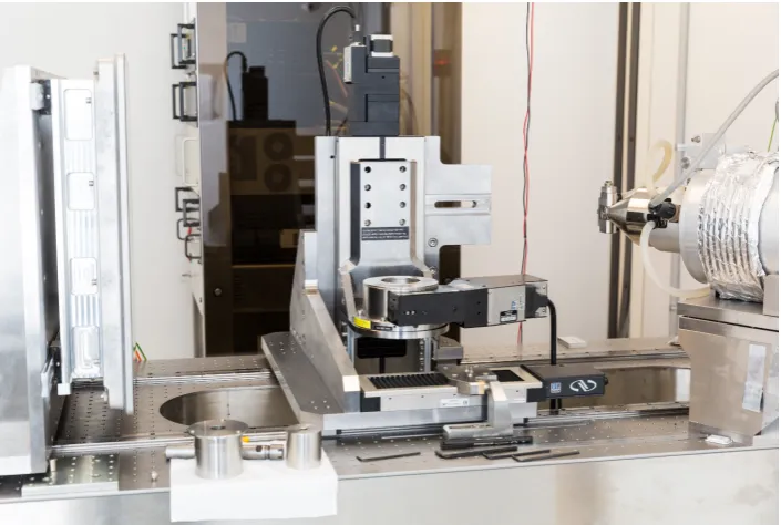
source at ANU CTLab, machine name: FEI4. . . 10 1.5 Photo of a Newport mechanical stage, in between the

detec-tor and the source, used at the ANU CTLab, (machine name: ANU1, see section 1.2.5). The background is the XPS motion controller that controls the movement of the stage. . . 11 1.6 A photo of an X-ray CT detector (Pixium RF 4343) used at the

ANU CTLab, machine name: ANU1. . . 13 1.7 X-ray images of a Sucrosic Dolomite rock with as same set-up

(a) and (b), taken with micro-CT at ANU. The source is set at 80 keV with 0.8 mm aluminium filter, and electron current of 100 µAmps towards a tungsten source target. The detector is

a Varian Flat Panel, each image takes 1.8 seconds accumulative exposure time, with a voxel size of 1.24 microns, with an object to source distance of 1.9 mm, and a camera length of 297.4 mm. Those images were taken by Dr. Michael Turner. . . 22 1.8 The difference in X-ray counts between the two images in Fig.

1.9 The line profile through the red line (drawn in Fig. 1.8): (top graph) through each image in Fig. 1.7; (bottom graph) through the difference image in Fig. 1.8. The line profile shows noise from 0-150 microns, and systematic error between 150-220 mi-crons. . . 23 1.10 A monochromatic plane wave propagates in the direction of

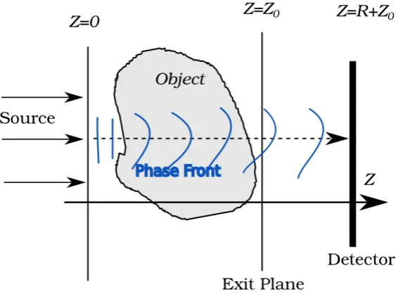
z-axis, through a scatter object in grey betweenz =0 and the exit plane z = z0, onto a detector atz = z0+R. The attenuating is shown in dotted line and phase shift is shown in blue. . . 50 1.11 Phase shift obtained from: (a) original phantom, (b) phase

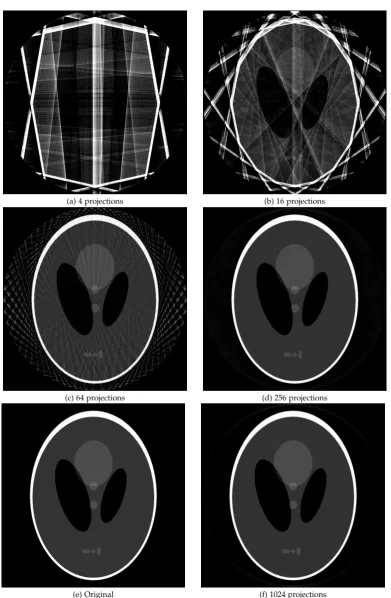
re-trieval with correct alignment, (c) phase rere-trieval with misalign-ment of 3 pixel horizontally and 5 pixel vertically. . . 71 1.12 Cone-beam reconstruction: FBP for (a) 4, (b) 16 (c) 64, (d) 256

and (f) 1024 projection angles, and (e) original phantom image. 75 1.13 Illustrate the helical trajectory in red, and the space filling

tra-jecotry in blue. . . 78

2.1 Comparing the radiographs between a point source and a non-point source. . . 86 2.2 Original image, RL and CG (50 iterations, optimal by L2 error

from the original (160 by 160 pixels). c[2013] ICTMS. . . 93 2.3 Filtered back-projection (FBP), RL with regularisation and CG

(64 iterations) with regularisation (160 by 160 pixels). c[2013] ICTMS. . . 93 2.4 Transverse movement along x-axis or y-axis of an impulse

ob-ject leads to the same convolution on the detector c[2014] SPIE. 97 2.5 Longitudinal movement along z-axis of an impulse object leads

to a different image on the detector c[2014] SPIE. . . 97 2.6 Coordinates used for the source and detector setup. . . 100 2.7 M-RL illustration diagram (not to scale). c[2015] IEEE. . . 110 2.8 M-RL process flow chart for each angle of projection. c[2015]

2.9 Original phantom for simulation, lower right quadrant of the central slice, with the red diagonal line indicates the line profile plotted in section 2.6.4.2 and 2.6.5.2. c[2015] IEEE. . . 114 2.10 Reconstruction using: (a) FBP, (b) RL and (c) CG method (lower

right quadrant of the central slice), under low cone-angle, with-out noise. c[2015] IEEE. . . 120 2.11 Reconstruction using: (a) FBP, (b) RL and (c) CG method (lower

right quadrant of the central slice), under medium cone-angle, without noise. c[2015] IEEE. . . 120 2.12 Line profile (over 64 pixels in horizontal axis, and “attenuation”

value in vertical axis) from the centre to the edge for low cone-angle, without noise. c[2015] IEEE. . . 121 2.13 Line profile (over 64 pixels in horizontal axis, and “attenuation”

value in vertical axis) from the centre to the edge for medium cone-angle, without noise. c[2015] IEEE. . . 121 2.14 Projection images obtained under high cone-angles: (a)

non-point source, (b) non-point source, (c) non-non-point source with RL correction, (d) non-point source with M-RL correction for the second reference slice from near the source. c[2015] IEEE. . . . 124 2.15 Reconstruction using: (a) FBP, (b) RL and (c) CG method (lower

right quadrant of the central slice), under high fan-angle, with-out noise. c[2015] IEEE. . . 125 2.16 Reconstruction using: (a) FBP, (b) RL and (c) CG method (lower

right quadrant of the central slice), under high fan-angle, with noise. c[2015] IEEE. . . 125 2.17 Multi-slice RL method, for high cone-angle, (a) without and (b)

with noise respectively. c[2015] IEEE. . . 125 2.18 Line profile (over 64 pixels in horizontal axis, and “attenuation”

2.19 Line profile (over 64 pixels in horizontal axis, and “attenua-tion” value in vertical axis) from the centre to the edge of the reconstructed object, for high cone-angle, with noise. c[2015] IEEE. . . 126 2.20 Second line profile (over 64 pixels in horizontal axis, and

“at-tenuation” value in vertical axis) from the centre to the edge for high fan-angles (with equal white band thickness), with noise. 127 2.21 Illustration of different X-ray sources, with the sample located

to the right of each source. c[2015] IEEE. . . 131 2.22 Ground Truth (GT) Reconstruction, with the centre and the

outer boxed region c[2014] SPIE. 3 mm diameter Sucrosic Dolomite rock. . . 134 2.23 Reconstruction using: (a) FBP and (b) RL method c[2014] SPIE. 135 2.24 Reconstruction using: (a) CG and (b) M-RL method c[2014]

SPIE. . . 136 2.25 A feature (each subimage is 90 by 90 voxels, or 370 microns) in

the centre region of (a) the GT reconstruction, and reconstruc-tion using: (b) FBP, (c) RL, (d) M-RL and (e) CG methods. CG has failed to produce a sharper image, RL and M-RL produce the same sharp image compared to FBP c[2014] SPIE. . . 137 2.26 A feature (each subimage is 90 by 90 voxels, or 370 microns) in

the outer region of (a) the GT reconstruction, and reconstruc-tion using: (b) FBP, (c) RL, (d) M-RL and (e) CG methods. CG has failed to produce a sharper image, RL and M-RL both pro-duced sharper images compared to FBP c[2014] SPIE. . . 137 2.27 Line profile through the centre region, CG result is removed as

2.28 Line profile through the outer region, CG result is removed as it did not converge. RL and M-RL produced sharper image compared to FBP, while M-RL is sharper than RL c[2014] SPIE. Horizontal axis is the pixel index over 30 pixels, and the vertical axis is the linear X-ray attenuation coefficient per voxel length ( 4.1 microns). . . 139

3.1 Original object showing [whole image]: (a) Compton signal (∝ R

ρdz) and (b) photoelectric signal (∝ R ρZ3dz), with the

numbering for different edges. The red dotted line is data used to draw the line profiles, and the blue boxes are used to subset the overall image for comparing phase retrieval results. . . 170 3.2 Original object [blue boxed (Fig. 3.1), subsets of the overall

image] showing: (a) Compton signal (∝ R

ρdz) and (b)

photo-electric signal (∝R

ρZ3dz). . . 172

3.3 Line profile of the normalised detected intensity for the second (reverse phase contast) edge at: (a) 30 keV, and (b) 60 keV. . . . 172 3.4 Direct material property estimation without phase retrieval [blue

boxed (Fig. 3.1), subsets of the overall image] showing: (a) Compton signal (∝R

ρdz) and (b) photoelectric signal (∝R ρZ3dz).173

3.5 Line profile of the direct material property estimation without phase retrieval showing: (a) Compton signal (∝ R

ρdz) and (b)

photoelectric signal (∝ R

ρZ3dz). Horizontal axis is over 80

pixels, at 2 microns per pixel. . . 173 3.6 Single material method showing: (a) Compton signal (∝R ρdz)

and (b) photoelectric signal (∝R

ρZ3dz). . . 174

3.7 Line profile of the single material method showing: (a) Comp-ton signal (∝ R

ρdz) and (b) photoelectric signal (∝ R ρZ3dz).

Horizontal axis is over 80 pixels, at 2 microns per pixel. . . 174 3.8 DCM showing: (a) Compton signal (∝ R ρdz) and (b)

photo-electric signal (∝R

ρZ3dz). . . 175

3.9 Line profile of DCM showing: (a) Compton signal (∝ R ρdz)

and (b) photoelectric signal (∝ R

ρZ3dz). Horizontal axis is

3.10 LIPR showing: (a) Compton signal (∝ R

ρdz) and (b)

photoelec-tric signal (∝ R

ρZ3dz). . . 176

3.11 Line profile of LIPR showing: (a) Compton signal (∝ R

ρdz) and

(b) photoelectric signal (∝ R

ρZ3dz). Horizontal axis is over 80

pixels, at 2 microns per pixel. . . 176 3.12 Direct material property estimation without phase retrieval

us-ing noisy radiographs [blue boxed (Fig. 3.1), subsets of the overall image] showing: (a) Compton signal (∝ R

ρdz) and (b)

photoelectric signal (∝ R

ρZ3dz). . . 178

3.13 Line profile of the direct material property estimation without phase retrieval using noisy radiographs showing: (a) Comp-ton signal (∝ R

ρdz) and (b) photoelectric signal (∝ R ρZ3dz).

Horizontal axis is over 80 pixels, at 2 microns per pixel. . . 178 3.14 Single material method using noisy radiographs showing: (a)

Compton signal (∝R

ρdz) and (b) photoelectric signal (∝R ρZ3dz).179

3.15 Line profile of the single material method using noisy radio-graphs showing: (a) Compton signal (∝ R

ρdz) and (b)

photo-electric signal (∝ R

ρZ3dz). Horizontal axis is over 80 pixels, at

2 microns per pixel. . . 179 3.16 DCM using noisy radiographs showing: (a) Compton signal

(∝ R

ρdz) and (b) photoelectric signal (∝R ρZ3dz). . . 180

3.17 Line profile of DCM using noisy radiographs showing: (a) Compton signal (∝R

ρdz) and (b) photoelectric signal (∝R ρZ3dz).

Horizontal axis is over 80 pixels, at 2 microns per pixel. . . 180 3.18 LIPR using noisy radiographs showing: (a) Compton signal

(∝ R

ρdz) and (b) photoelectric signal (∝R ρZ3dz). . . 181

3.19 Line profile of LIPR using noisy radiographs showing: (a) Comp-ton signal (∝ R

ρdz) and (b) photoelectric signal (∝ R ρZ3dz).

Horizontal axis is over 80 pixels, at 2 microns per pixel. . . 181 3.20 Normalised radiographs of a diamond with magnesium alloy

3.21 Log ratio of misaligned projections: (a) shows the whole field of view, with the blue box indicating the area shown in (b). There areghost shadowin (a) and (b) show the number of pixels in misalignment. . . 189

3.22 Log ratio of correctly aligned projections: (a) shows the whole field of view, with the blue boxed area shown in (b). There are no apparent ghost shadow, therefore the correct alignment between projection of different energies can be inferred. . . 190

3.23 Compton signal (∝R

ρdz, threshold to between 0.0 (black) and

6.0 (white)mg/mm2) of the diamond and magnesium on glass post: (a) no phase retrieval, (b) single material, and (c) LIPR methods. The blue box shows the zoomed in area for the next figure. . . 192

3.24 Zoomed in (top left blue square of Fig. 3.23 (a), threshold to between 3.0 (black) and 5.5 (white) mg/mm2 for clear visual-isation), Compton signal (∝ R

ρdz) of the diamond and

mag-nesium on glass post: (a) no phase retrieval, (b) single mate-rial, and (c) LIPR methods. A horizontal line profile is drawn through the crack of the diamond. . . 193

3.25 Line profile (Over 50 pixels, 1.3 microns per demagnified pixel) through crack in the diamond phase edge to compare: no phase retrieval, single material, and LI-PR method. To show the Comp-ton signal in the no retrieval, single material and LI-PR re-trieved the Compton information. Horizontal axis is pixels. . . 194

3.26 Photoelectric signal (∝ R

ρZ3dz, thresholded between 0 (black)

3.27 Zoomed in (top left blue square of Fig. 3.26 (a), thresholded between 0 (black) and 1500 (white) Z3mg/mm2 for clear visu-alisation), photoelectric signal (∝ R

ρZ3dz) of the diamond and

magnesium on glass post: (a) no phase retrieval, (b) single ma-terial, and (c) LIPR methods. . . 196 3.28 Line profile (Over 50 pixels, 1.3 microns per demagnified pixel)

through the diamond/Magnesium reverse phase contrast edge to compare: no phase retrieval, single material, and LI-PR method. To show the photoelectric signal in the no retrieval, single ma-terial and LI-PR retrieved the photoelectric information. Hori-zontal axis is pixels. . . 196 3.29 Effective atomic number (Z, thresholded to between 0 (black)

and 12 (white) Z) of the diamond and magnesium on glass post: (a) no phase retrieval, (b) single material, and (c) LIPR methods. The blue box shows the zoomed in area for the next figure. . . 198 3.30 Zoomed in (top left blue square of Fig. 3.29 (a), thresholded

to between 4 (black) and 10 (white) Z for clear visualisation), effective atomic number (Z) of the diamond and magnesium on glass post: (a) no phase retrieval, (b) single material, and (c) LIPR methods. . . 199 3.31 Line profile (Over 50 pixels, 1.3 microns per demagnified pixel)

through crack in the diamond phase edge to compare: no phase retrieval, single material, and LI-PR method. To show the cal-culated effective atomic in the no retrieval, single material and LI-PR retrieved the Compton information. Horizontal axis is pixels. . . 199

4.1 Plot of space filling (based on Eqn. 4.1), single helical and dou-ble helical trajectories. L = W = 256 voxels, andV = R =128 voxels (as discussed in section 4.1). . . 206 4.2 Compare the windowing between our SF multi-grid

4.3 SF MGR of limestone (horizontal slice) at 1/4 scale . . . 215 4.4 SF MGR of limestone (horizontal slice) at 1/2 scale. . . 215 4.5 SF MGR of limestone (horizontal slice) at full scale. . . 216 4.6 SF MGR of sandstone and limestone (part of vertical slice): (a)

Without using windowing, and (b) Using the Colsher’s Laplace filter rather than using the correct filter as outlined in Eqn. 4.5. 218 4.7 Sandstone and limestone (part of vertical slice): (a) SF MGR

applying the constant vertical angle windowing and the correct filtering kernel as outlined in Eqn. 4.4 and 4.5. (b) DH KFBP reconstruction. . . 219 4.8 Zoomed in region of SF MGR of sandstone and limestone (part

of vertical slice): (a) Without using windowing, and (b) Using the Colsher’s Laplace filter rather than using the correct filter as outlined in Eqn. 4.5. . . 220 4.9 (a) Zoomed in region of the SF MGR (vertical slice): using

2.1 Quantitative results for relative noise, relative sharpness, rela-tive signal to noise, and L2error from the original. To compare different source deblurring methods c[2013] ICTMS. . . 94 2.2 Computational cost of FBP, RL, M-RL and CG (relative to FBP).

c

[2015] IEEE. . . 117 2.3 Quantitative results for the central slice of the reconstructed

object, calculated according to subsection 2.6.3. c[2015] IEEE. . 127 2.4 Relative quantitative results c[2014] SPIE. . . 140

3.1 L2 error for the noiseless case: for no retrieval, single material, DCM, and my LIPR methods. Edge error is obtained on the edge with a width of 4 pixels. Edges 4 and 6 are not shown, since they contain no extra information. . . 176 3.2 L2 error for the noisy case: for no retrieval, single material,

DCM, and my LIPR methods. . . 182 3.3 Proportion of X-ray energy for each imaging setup (generated

Introduction and Background

Optical imaging is the art of measuring the interaction between light and an object, in a way that helps us understand that object. An imaging process consists of light, an object, a detector, and a processing device. The object disturbs the light field, thereby embeds information onto the light field, and the intensity of the light field is measured by the detector.

Visible light only interacts with the surface of an optically opaque object, so a more penetrating light or a physical probe is needed to obtain informa-tion regarding the internal and composiinforma-tion of the object. Knowing the inter-nal structures of the object is fundamental in understanding many physical, geological and biological processes. X-rays have a high penetrating power, so there are interactions with the internal structure of objects. Section 1.1 shows why X-rays are used for imaging, and the progression of X-ray imaging tech-nology through history to today’s Computed Tomography (CT) system used at ANU CTLab.

The X-ray micro-CT imaging system consists of an illuminating X-ray source, an object of interest, one or more stages to translate and rotate the object, and an X-ray detector. X-rays generated from the source are scat-tered when passing through the object and then propagates to the detector. These propagated X-rays are imaged by measuring the intensity at the X-ray detector. I describe the fine-focus X-ray micro-CT set-up used at ANU in comparison to a few other systems, as well as progresses and applications of X-ray CT in section 1.2.

im-provement in source deblurring in chapter 2 and phase retrieval in chapter 3. These two chapters form the main body of my original work.

I divide the rest of the background of X-ray micro-CT into the following sections: optimisation problems (section 1.3), modelling of X-ray waves (sec-tion 1.4), X-ray propaga(sec-tion approxima(sec-tion (sec(sec-tion 1.5), state-of-the-art phase retrieval algorithms (section 1.7), X-ray and object interaction (section 1.6), CT reconstruction with circular trajectory (section 1.8), and its applications (sec-tion 1.9).

The optimisation problems in section 1.3 present fundamental statistical and mathematical tools we use to form a physical model of the X-ray waves propagation through free space and matter. I present the statistical maximum likelihood inference and show that optimising the statistical likelihood for a normal distribution is equivalent to a metric norm optimisation. We then present methods to solve this metric norm optimisation.

Section 1.4 presents a physical model of light propagation, in particular the X-ray wave propagation in free space and through matter. In this section I present equations characterising the X-ray propagation on the temporal and spatial scale of a typical lab-based X-ray CT system.

Section 1.5 studies and models directional X-ray propagation towards the detector, by combining the results from the optimisation problems and mod-elling of X-ray in section 1.3 and 1.4 respectively. This section presents a forward projection approximation through matter (useful for CT reconstruc-tion), and the transport of intensity equation through free space (useful for phase retrieval).

Section 1.6 investigates different types of X-ray scattering in the object, and discusses the relevance to micro-CT systems. I quantify the attenuation and phase shift coefficients within the object in terms of X-ray energy, and the object properties of density and atomic number.

Section 1.8 presents a filtered back-projection CT reconstruction algorithm and an iterative reconstruction algorithm for projection data acquired using a circular X-ray source trajectory. This reconstruction algorithm outputs the X-ray attenuation of the object, and I use this reconstruction algorithm to demonstrate the sampling sufficiency requirements.

In section 1.9, I will outline the assumptions made in section 1.7 and 1.8 that could be invalid for lab based micro-CT system, and the corresponding computation or hardware remedies that could eliminate or reduce the effect of such break downs in assumptions.

1

.

1

Why X-rays?

X-rays were discovered by Wilhelm C. Röntgen in 1895, who received the first ever Nobel Prize in Physics. The famous image of his wife’s hand with the ring [1] is considered to be the first medical X-ray image ever taken, and that has demonstrated the potential of using X-rays to image internal structures. He created X-rays by accelerating electrons from a cathode to an anode with a potential difference (or voltage) ranging from a few keV to 100 keV. Upon impact with the anode, some of the energy from the electrons are converted to X-ray photons.

1

.

1

.

1

Development of X-ray Computed Tomography (CT)

X-ray CT is concerned with reconstructing an object from multiple projec-tions of the object and it is a combination of two fields: X-ray imaging and computed mathematical inversion reconstruction.

As outlined above, X-rays were first discovered in 1895 by Röntgen [1], and the very first X-ray radiograph image of his wife’s hand demonstrated the possibility of using X-rays to image internal structures. Projectional radio-graphy was invented by the Italian radiologist Alessandro Vallebona in the 1930s by taking X-ray radiograph images from multiple angles, this allows 3-D information to be obtained from those 2-D X-ray images [2].

Computed Tomography (CT) came much later; the direct reconstruction technique was first applied to radio astronomy in the 1960s and was devel-oped by Bracewell and Riddle [3]. It was first put into clinical use in medical-CT in the early 1970s. At that time, a clinical scan could produce images from a circular scan that were 100 by 100 pixels. By the end of 1970s, CT machines could produce images that were 512 by 512 pixels. By the late 1980s, it only took 3 seconds to produce an image of the size of 1024 by 1024 pixels. Im-provement continued through the 1990s, multi-slice detectors with the best CT machine was capable of returning an image with 4-slices of images[4; 5].

CT technology continues to improve by having more image pixels, and higher resolution. In 1982, the first micro-CT was invented and built by Elliott and Dover [6], their micro-CT achieved a pixel size of about 20 microns. In the 1990s, micro-CT systems have become commercially available [7]. In 2016, the state-of-the-art micro-CT scanner with the use of the supercomputer at Australian National University can produce a quality 3072 by 3072 by 3072 to 18000 voxels 3D-image [8]. I will discuss X-ray micro-CT in section 1.2.

1

.

2

X-ray Micro-CT System and Comparison

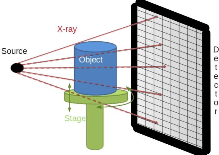
consists of four parts: (1) an illuminating X-ray source (see section 1.2.1), (2) an object being imaged (see section 1.2.2), (3) one or more stages that translate and/or rotate the object relative to the source and detector (see section 1.2.3), and (4) an X-ray detector to measure the X-ray intensity after passing through the object (see section 1.2.4). For an illustration of a CT setup, see Fig. 1.1.

Fig. 1.1: An illustration of an X-ray CT setup.

1

.

2

.

1

X-ray Source

The X-ray source is used to generate X-ray photons, some of these photons then travel through the object onto the detector. See Fig. 1.1 for the relative position of the X-ray source in a CT system. Current state-of-the-art X-ray sources include lab based reflection source, lab based transmission source, and synchrotron source.

(braking radiation) effect [9; 10; 11]. Only a small fraction (about 1%) of the kinetic energy of the electrons are transformed into X-ray photons, while the rest are transformed into heat. This heat can damage the target, and is a topic for future discussion.

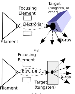
For an illustration diagram of transmission and reflection source, see Fig. 1.2 (drawn after consultation with Dr. Levi Beeching).

In a synchrotron source (see section 2.2 of X-ray Data Booklet [12] for an in depth background), X-ray photons are generated by bending or wiggling a beam of electrons travelling near the speed of light. When the travelling path of electrons are bent, high energy photons (in this case, X-ray photons) are produced in the same direction as the original path of the electron beam.

In terms of target and filament material, there are three subcategories for reflection sources: stationary target material, rotating anode, and liquid metal jet sources [13]. Many other materials are used in place of tungsten, such as molybdenum and silver used as target and filament, where LaB6is only used as filament.

For micron scale imaging, the incident electrons need to be focused and filtered to a micron sized spot on the target material, we call this a micro-focused X-ray source. Since not all X-rays are generated on the surface, a thin target material reduces the source spot volume size. Since the target material for transmission sources is generally much thinner than the target material for a reflection source, therefore the spot volume size for transmission source is smaller (see Fig. 1.4 for a photo of a transmission source). For ANU CTLab, this micro-focus set-up generates an X-ray source that is close to a point for imaging objects that requires resolution less than 10 microns (see section 1.2.5 for specifications).

This micron sized source spot reduces the penumbral blurring at the de-tector when using the fine-focus set-up at the ANU CTLab. Penumbral blur-ring is a limiting factor in the imaging resolution of the fine-focus micro-CT system, and this is discussed in depth in section 1.9.2.

(top)

(bottom)

Fig. 1.2: An illustration of a micro focus source: (top) reflection source, (bot-tom) transmission source.

of the micro-focus source. The problem of a transmission micro-focus X-ray source is the small focus spot size, therefore the source could only operate at lower electron intensity (and with lower X-ray intensity being generated) to prevent the melting of the filament or the target from the electron beam. The maximum thermal constraint for power per focus spot radius at melt-ing is in the range of 0.7-1.5 W/µm for tungsten (≈ 1.3W/µm), copper or

molybdenum filament [14]. For LaB6 filament, a current of 3-5 times more than tungsten can be achieved [15] under the micro focus setting due to a smaller work function. However, the generated X-ray intensity is still under the thermal constraint of the micro-focus source.

and into a bigger target volume. So at ANU CTLab, for imaging large objects when the required resolution is 10 microns or larger, a reflection source is used due to the higher X-ray flux (see section 1.2.5 for specifications).

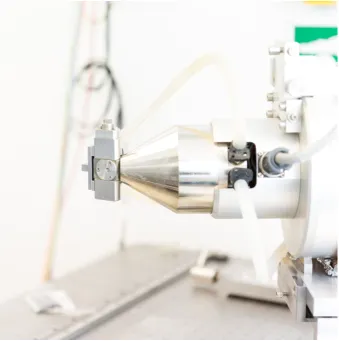
Fig. 1.3: A photo of a reflection micro focus source at ANU CTLab (machine name: ANU1, see section 1.2.5).

1

.

2

.

2

Imaged Object

X-rays generated by the source (see section 1.2.1) scatter through the object before being recorded at the detector (see section 1.2.4). Objects from the size of a protein molecule [17] to the size of an entire truck [18] have been imaged by X-ray imaging. Depending on the X-ray imaging system, constraints such as object size, atomic composition and density are placed on the object to obtain decent signal to noise ratio and artefacts free images.

When X-ray photons pass through an object, some of them are absorbed or scattered away from the detector, and some of them are bent slightly and still hit onto the detector [19; 20]. When the object absorbs or scatters the X-ray away from the detector, this is called X-X-ray attenuation. When the object bends the path of the X-ray, this is called refraction.

To obtain decent signal-to-noise-ratio (SNR), a good fraction of the X-ray photons through sample must reach the detector, and a good fraction of the X-ray photons must be attenuated or refracted by the sample.

The amount of X-ray attenuation depends on both the sample and the X-ray energy, this will be explored in detail in section 1.6. Generally high energy X-rays (being more penetrative) are used to image large, dense and high atomic numbered samples. While low energy X-rays are used to image small, light and low atomic number samples, due to the need for X-ray inter-action with the object. The optimum sample attenuation can in principle be calculated [21]. Since each X-ray source can only generate X-rays in a certain energy range, this places constraint on the size, density and atomic compo-sition of the object being imaged to ensure decent signal to noise ratio in a reasonable time.

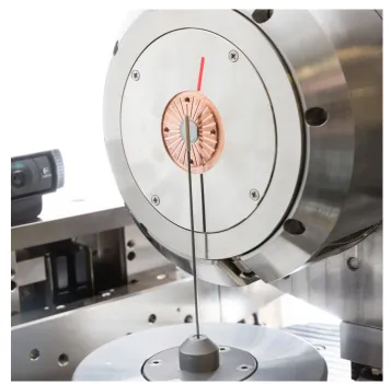
Fig. 1.4: A photo of an object mounted on post in front of a transmission source at ANU CTLab, machine name: FEI4.

1

.

2

.

3

Stage

To form a 3-D CT reconstruction of the object, we need to image the object from various angles [23]. This is achieved by translational and rotational movement of the object, relative to the source and detector, in between imag-ing at each angle and at each height.

These relative movements are achieved differently for different CT sys-tems. For medical CT, this relative translation and rotation is performed by the rotating source and detector around the translated patient being scanned. For conventional micro-CT, this relative translation and rotation is obtained by fixing the object onto a stage, and the object is rotated and translated by the stage while keeping the source and detector stationary.

There are a few trade-offs between different stages for conventional CT: precision of movement, weight and size restrictions on the object, maximum travel distance, and cost. The precision of movement is important, as errors in motion of the stage would cause motion artefacts in the reconstruction [24], in such cases sophisticated algorithms are needed to correct this artefacts [25].

Fig. 1.5: Photo of a Newport mechanical stage, in between the detector and the source, used at the ANU CTLab, (machine name: ANU1, see section 1.2.5). The background is the XPS motion controller that controls the movement of

1

.

2

.

4

Detector

After the X-ray photons are transmitted through or scattered by the object, they are recorded by the detector. The detector is used to measure the X-ray intensity at the detector plane, using chemical or physical reactions to form an image. See Fig. 1.1 for an illustration about where the detector is integrated in the whole X-ray CT system. Commonly used X-ray detection systems include: X-ray film, direct semiconductor detector, and scintillator plus semiconductor detector. This subsection investigates the each X-ray imaging method, and a comparison between the different methods.

X-ray film uses photographic plates that are sensitive to X-rays, and records the X-ray intensity hitting the plate. It typically has four layers: cellulose triacetate or polyester base layer, adhesive layer, silver halide and gelatine emulsion layer, and a protective layer [26]. When the X-ray film is exposed to X-ray photons, the emulsion layer produces silver ions and electrons, and the electrons would attract the silver ions, and form clumps of metallic silver (in black colour). It is cheapest X-ray detectors comparing to electronic X-ray detectors, and commonly used in dentistry. However, the film could only record one X-ray image, and the existence of digital archiving makes the film less useful as a storage system.

Direct semiconductor detector, first developed in 1970s, converts X-ray photons into electron-hole pairs in the semiconductor, and these electron-hole pairs are collected by measuring the current to detect the X-rays at each de-tector pixel [27]. Direct semiconductor dede-tectors are commonly based on cad-mium telluride (CdTe) and its alloy with zinc. Other direct semiconductors use materials such as silicon, diamond or germanium. Direct semiconductor detectors often requires advanced cooling, and are generally expensive.

the scintillator plus amorphous silicon semiconductor detectors, see section 1.2.5 for detailed specifications of detectors used in our CT lab.

Fig. 1.6: A photo of an X-ray CT detector (Pixium RF 4343) used at the ANU CTLab, machine name: ANU1.

One important aspect of CT setup that can be overlooked is the space between the object and detector. For a fine focus micro-CT setup, there is a geometric magnification by having a short distance between the source and the object in comparison to the distance between the source and the detector. This geometric magnification (in the region of 10-1000 times) allows detector pixels to be much larger than the imaging resolution needed for the object.

1

.

2

.

5

ANU CTLab System

All the experimental data presented in this thesis was collected at the ANU CTLab. In this subsection, I describe the X-ray source, objects imaged, de-tectors and stages used at the ANU CTLab. At ANU CTLab, they image a range of material composition and object size. They have imaged geological rock samples, biological samples, in situ flow experiments [29], and material science structure samples.

At ANU CTLab, there are three X-ray CT machines: ANU1, ANU2 and FEI4. Each of them have very different X-ray sources and therefore different capabilities of imaging.

1.2.5.1 ANU CTLab X-ray Source

Each CT machine at the ANU CTLab uses a transmission or reflection micro-focus X-ray source with a stationary piece of tungsten as the target material, see Fig 1.2 for an illustration. At the ANU CTLab, electrons are generated from the filament accelerated to a certain voltage, the electrons are acceler-ated toward the target at particular kinetic energy between 20-180 keV. The accelerated electrons are focused by the focusing elements onto a spot on the target material. The source spot size are in the range of 0.3-10 microns, the exact source spot used depends on the amount of X-ray flux needed, electron energy, the filament, and the target material geometry.

For transmission source used on ANU2 and FEI4 CT machines, the target tungsten has a thickness of 1 and 3 microns respectively, with the source spot size between 0.3 to 3 microns (depend on the focus mode). For the transmission source configuration, a diamond window is used to support and cool the thin tungsten target and support the vacuum needed for the X-ray source. While for reflection source used on ANU1, the target tungsten is a block of tungsten metal with a flat reflection surface, the source spot size is around 5-10 microns. For the reflection source, Beryllium window is used to support the vacuum needed for the X-ray source, and the block of tungsten can support and dissipate heat due to its 3-D geometry.

filament on the ANU2 CT machine. A tungsten filament is more economical compared to LaB6 filament, however LaB6 lasts longer, and can focus the electrons onto a spot size of 0.3 micron compared to 1 micron for the tungsten filament. Common target include tungsten (atomic symbol W), copper or molybdenum, however in our CT lab we only use the tungsten target. For a photo of the source used at ANU CTLab, see Fig. 1.3.

For each X-ray source, there are some modes of focusing with correspond-ing trade off in X-ray flux. For the ANU1 machine, the electrons are focused to a spot size of approximately 3 microns, with relative flux of approximately 40 times compared to ANU2 S mode. For ANU2 machine, the S and M mode are commonly used, it focus the source to a spot size of approximately 0.3 and 0.7 micron respectively, with relative flux of approximately 1 and 4 re-spectively times compared to ANU2 S mode. For FEI4 machine, the S, M and L mode can focus the source to a spot size of approximately 1, 1.5 and 3 microns respectively, with relative flux of approximately 4, 10 and 20 respec-tively times to ANU2 S mode.

From those specifications on the source, it is evident that ANU1 is a high flux X-ray source, while ANU2 is a nano-focus source, and while FEI4 is a one-micron-focus source. To optimise the resolution and signal to noise ratio of the X-ray image, we typically choose source spot size to be equal to or smaller than the voxel width of the object, and picking an X-ray energy where around 5-40 percent of the X-rays gets attenuated through the sample (this percentage could be calculated [21]).

The X-ray source on ANU1 is Nikon (www.nikonmetrology.com), and the X-ray sources on FEI4 and ANU2 are Hamamatsu (www.hamamatsu.com).

1.2.5.2 ANU CTLab Object Imaged

by the ability to secure the object onto the stage, and sample rigidity.

In ANU CTLab, we typically image geological, biological, and material science samples. The composition of object that could be imaged is restricted by the X-ray energies from our source. Since our source could generate X-ray in the range between 20-180keV, as a quick guide for a solid object with a den-sity around 0.5-4 relative to water (or g/cm3), only effective atomic number between 3 and 47 could be imaged with a decent signal to noise ratio. Hy-drogen and helium are not attenuating enough for the X-rays we generate, so there would be very little contrast. A solid with atomic number much higher than silver (silver has an atomic number of 47) is becoming too attenuating for the X-rays we generate to penetrate through. For a detailed attenuation calculation, see section 1.6.2 and 3.2.1.

ANU1 has a high flux X-ray source, therefore it is designed to image more attenuating object with diameter around 5 to 200mm, with resolution in the range of 3 to 100 microns. The whole object has to fit in the detector’s field of view, and each detector has a fixed number of pixels, so there is an inverse relationship between sample diameter and imaging resolution.

ANU2 has a nano-focus X-ray source, this CT machine is focused on imag-ing less attenuatimag-ing object with diameter 0.5-3mm with a 0.25-1.5 micron res-olution.

FEI4 has a one-micron-focus X-ray source, this CT machine is designed to image medium attenuating object with diameter 2-20mm with about 1-10 micron resolution.

1.2.5.3 ANU CTLab Detector

microns, so this is not an area that need improved precision of movement in the stages.

For ANU1, we use a Pixium RF 4343 X-ray detector made by Thales (www.thalesgroup.com). The scintillator is a Pixium, made up of Caesium Iodide. The imaging receptor has pixel size 148 microns, the X-ray imag-ing array has 2874 by 2840 pixels or 43 by 43 centimetres. It is designed to detect X-rays in the 40-150 keV range. There is a 0.5% lag in X-ray hitting the scintillator and fully registered by the detector for a frame (at maximum frame rate), this leaves an afterglow of 0.5% in the next frame. The images are sent by Camera Link and LVDS Parallel, with communication provided by Ethernet, and DC input power 110/220-240 V. The detector has an overall dimension of 508 by 518 by 80.9 mm, and weighs 25 kg, while the processing unit has a dimension of 320 by 483 by 177 mm, and weighs 13 kg. The cooling of the detector is achieved by air flow cooling.

by the detector for a frame (at maximum frame rate), this leaves an after-glow of 0.5% in the next frame. The maximum readout speed is 4 frames per second at the full resolution, and the scan method is progressive. The data are outputted by LVDS and CameraLink. It requires a power supply of 21-33 V, with a nominal power consumption of 54 watts and a peak power consumption (during initialisation) of 68 watts.

1.2.5.4 ANU CTLab Stage

At ANU CTLab, we use two types of stages: mechanical and air-bearing stages. The mechanical stages we use are Newport (see the photo in Fig 1.5), which are controlled using the Newport XPS motion controller. The air-bearing stage we use is made by Aerotech. If a particular accuracy is not critical for our CT system, we would take the manufacture’s accuracy statistics, as the case for ANU1. When a particular accuracy is critical for our CT system, such as ANU2 and FEI4, a quality testing report has been prepared.

For ANU1, the vertical translational stage is a Newport MTM250PP; it has 250 mm of vertical travel. According to the manufacturer’s statistics, the translational stage has a repeatability error of 3 microns, an on axis error of 5 microns. In terms of angular accuracy, it is within 40 µRad for both the

yaw and pitch. The rotational stage is a Newport RV120; it has 360 degrees of freedom of rotation. According to the quality report, the rotational stage has a repeatability error of 10µRad, an on axis error of 3.9 microns, and absolute

position error of 4.3 microns. All the data regarding the ANU1’s stage is from Newport’s manufactures website.

error of 1.9 µRad, and an absolute error of 7.7 µRad.

For FEI4, the vertical translational stage is a Newport MTM100; it has 100 mm of vertical travel. According to the quality testing report, the translational stage has a repeatability error of 0.3 microns, an on axis error of 1.6 microns, and an absolute position error of 7.9 microns. In terms of angular accuracy, according to the manufacture, it is within 40µRad for both the yaw and pitch.

For the rotational stage is a Newport RV160; it has 360 degrees of freedom of rotation. According to the quality testing report, the rotational stage has a repeatability error of 4.6 µRad, an on axis error of 3.9 microns, and absolute

position error of 4.3 microns.

Here, we want to mention that Aerotech’s air-bearing stages are by far the most accurate ones, and they are considerably more expensive than the Newport’s mechanical stages.

1

.

3

Imaging Optimisation Problems

Optical imaging set-ups allow the user to acquire data by measuring a light wave after interacting with an object: this is called the imaging process. A mathematical and statistical framework is required to model this optical imaging set up, such as the micro-CT in the ANU CTLab (see section 1.2.5).

1

.

3

.

1

Statistical Modelling

A measurement of a random process is a sampling from a statistical distri-bution. This subsection investigates the modelling of such a measurement process. Consider taking two images while keeping all conditions as similar as possible: i.e. attempting to have the same X-ray incident illumination, ob-ject and detecting set-ups. The outcome of the two images would likely be different, because most imaging is not a deterministic process due to noise, and systematic error in the imaging process. The noise and systematic er-ror could include: Gaussian noise due to the combination of many different noises (as a consequence of central limit theorem to be explained in section 1.3.1.2), quantum shot noise due to the discrete nature of electric charge or photons, and salt-and-pepper noise due to the existence of defect pixels on the detector. For a more complete account of the statistical nature of the noise, see [30; 31; 32].

For imaging, the interaction process between light and object, and the sub-sequent detection by the detector are all non-deterministic random processes. For example, Fig. 1.9 shows the line profiles of the X-ray images, and the difference between the two line profiles.

It is interesting to see some of the differences of X-ray intensity count at the detector due to unstructured artefacts (see the area on the left of thewhite vertical line in Fig. 1.8 and line profile Fig. 1.9), while some of the differences are structured artefacts (see the white vertical linein Fig. 1.8).

For unstructured artefacts, such as the quantum shot noise at the detector and the source due to statistical quantum uncertainty of the electrons or X-ray photons respectively, we need to increase the total accumulative exposure time to reduce this noise or uncertainty (see a statistical treatment in section 1.3.3).

(a) (b)

Fig. 1.7: X-ray images of a Sucrosic Dolomite rock with as same set-up (a) and (b), taken with micro-CT at ANU. The source is set at 80 keV with 0.8 mm aluminium filter, and electron current of 100 µAmps towards a tungsten

source target. The detector is a Varian Flat Panel, each image takes 1.8 seconds accumulative exposure time, with a voxel size of 1.24 microns, with an object to source distance of 1.9 mm, and a camera length of 297.4 mm. Those images

were taken by Dr. Michael Turner.

Fig. 1.8: The difference in X-ray counts between the two images in Fig. 1.7. Thewhite vertical linein the first quarter of the image is a structured difference due to misalignment, where the difference on the left of the white vertical line

Fig. 1.9: The line profile through the red line (drawn in Fig. 1.8): (top graph) through each image in Fig. 1.7; (bottom graph) through the difference image in Fig. 1.8. The line profile shows noise from 0-150 microns, and systematic

1.3.1.1 Poisson Distribution

Imaging at each detector pixel can be modelled by a statistical distribution. We consider a rare event model, where for a very short period of time, the probability of a single event happening is proportional to the length of the time interval. Also we assume no two events can occur at the same time. Lastly, under the semi-classical model [30], we assume the system has no memory, so what happens in the previous time intervals has no effect on the probability of something happening in any other time intervals.

Detector pixels are usually calibrated to operate in this manner, in the ab-sence of special circumstances. These special circumstances could include, for example: pileup of photons [33], defective pixels [34], pixel memory due to previous exposures, or over exposure in one accumulation. Without these special circumstances, the detector would be an imaging system that mea-sures the cumulative photon arriving events (by measuring the X-ray inten-sity) in a time period, and detection events are time independent [35]. There-fore, we can use a mixture of Gaussian and Poisson distribution to model this imaging system for the sum of measured photon arriving events in a given length of time.

1.3.1.2 Central Limit Theorem

For sufficient photon counts, there are enough independent observations from a statistical distribution to satisfy the condition for the central limit theorem (CLT). The CLT allows us to use a normal distribution to approx-imate a sum of Poisson and other distributions. The CLT has been studied extensively [36] since first being postulated by Abrahm de Moivre in 1733. However, it was in 1901 Aleksandr Lyapunov first defined and proved the CLT mathematically.

The Lyapunov CLT (more general than what is required here, see Billings-ley [37]) states: SupposeX1,X2, ... is a sequence of independent random vari-ables, each with meanµi and standard deviation σi. Let

s2_n =

n

∑

If for some δ>0, the Lyapunov’s condition is the following equation:

lim n→∞

1

s2+δ

n n

∑

Eh|X_i−µi|2+δ

i

=0. (1.2)

If Lyapunov’s condition is satisfied, then the sum of (Xi−µi)/sn con-verges in distribution to a standard normal random variable, as n goes to infinity:

1

sn n

∑

(Xi−µi) d

−→ N(0, 1). (1.3)

For n identical independent Poisson distributions with mean µ = λi = λ

for all i and standard deviation σ =

√

λ, we check for Lyapunov’s condition

forδ =1:

s2_n =

n

∑

σ_i2 =nλ. (1.4)

Since the mean and the third central moment of a Poisson distribution are

both λ: _n

∑

Eh|X_i−µi|2+δ

i =

n

∑

Eh|X_i−λ|3 i

=nλ. (1.5)

Therefore, we have the Lyapunov’s condition satisfied by:

lim n→∞

1

s2+δ

n n

∑

Eh|X_i−µi|2+δ

i

= lim

n→∞

1 ∑n

i=1(λi)1.5 n

∑

[λi]

= lim

n→∞ 1

n0.5

λ0.5 (1.6)

=0.

The Lyapunov’s CLT was used because it applies for n independent (not necessarily identical) Poisson distributions, with parameters λi that are not the same for all i, but there exist a value k ∈ R+ _where λi

of Eqn. 1.6 to obtain:

0≤_n→∞lim 1

[∑n_i=1(λi)]1.5 n

∑

(λi)

≤ lim n→∞

k1.5 (nλi)0.5

(1.7)

=0,

whereicould be any value between 1 andninclusive. The optimaliis chosen by finding isuch that λi ≥λj for any j.

Since the Lyapunov’s condition is satisfied (see Eqn. 1.7), therefore the sum of n independent Poisson distributions converges to a normal distribu-tion as n → ∞. Eqn. 1.7 provides an upper bound on how fast Lyapunov’s

condition is satisfied for the sum of independent (but not necessarily identi-cal) Poisson distributions.

Here, we comparenindependent (not necessarily identical) Poisson distri-butions with mean equal to λi (i ∈ {1, 2, ...,n}) withm independent identical Poisson distributions with each mean equal to λ, where λ = min(λi). The sum of former distributions (the non-identical ones) would requiresn =k1.5m

to satisfy the Lyapunov’s condition to the same extent as the latter distribu-tions (the identical ones). This would satisfy the Lyapunov’s CLT for the case when multiple exposures are taken under slightly different conditions where the mean (λi) of the Poisson distributions are slightly different between

expo-sures. So, if there is a maximum of 5% variation (k =1.05) of expected counts for different exposures to be accumulated together, then there is a need to take 7.6% more exposures (k1.5−1 = 0.076) to satisfy the Lyapunov’s con-dition for CLT to the same extent compared to having n independent and identical Poisson distributions.

This 5% variation of expected counts between different exposures could occur if the source intensity varies through the individual exposures, or the detector efficiency changes during the imaging process.

Un-der Lyapunov’s condition, we demonstrated that this can be approximated by a normal distribution. In section 1.3.3, I will show that a normal distribution’s maximum likelihood function could be optimised by minimising in a metric norm (introduced in section 1.3.2).

1

.

3

.

2

Metric Norm

This subsection explains the definition of a norm space, and commonly used norms. This lays a foundation for the next subsection regarding normal dis-tribution and metric norm error minimisation. The L2 norm is commonly used, as it measures the Euclidean distance between two points.

There are three axioms needed for a function mapping a vector space to a real number to be called a metric norm [38]: scalability, the triangle inequality and separate points. Given a vector space V over a field C of the complex numbers, a metric norm on V is a function f : V → R with the following properties:

For all a∈ Cand all~u,~v ∈V, it satisfies the scalability condition:

f(a~v) =|a|f(~v). (1.8)

It satisfies the triangle inequality:

f(~u+~v)≤ f(~u) + f(~v). (1.9)

It satisfies the separate points condition: if

f(~v) = 0, (1.10)

then~vis the zero vector.

Those three axioms also imply non-negativity: f(~v) ≥0 for all~v ∈ V. The commonly known metric norms areL1,L2and L∞, which corresponds to:

k~xkp =

∑

|x_i|p !1/p

for p =1, 2, and limp→∞ respectively.

The L1norm is the sum of absolute distance in each dimension, and min-imising the L1 norm error would put the same focus on each dimension ir-respective of absolute error. The L2 norm measures the Euclidean distance, and minimising the L2 norm error would put more focus on the dimension with larger error. The L∞ norm obtains the maximum absolute value in the vector, and minimising the L∞ norm error entirely focuses on the dimension with the largest absolute error.

L0 works by counting the number of non-zero element in a vector. How-ever, it is technically only a semi-norm, as it violates the scalability condition in Eqn. 1.8.

This subsection has presented the definition of a norm, and the commonly used norms, including the L2 norm. In the next subsection, I will combine the results of this and the previous subsection to show that maximising the likelihood of a normal distribution is equivalent to minimising the L2 norm.

1

.

3

.

3

Normal Distribution and

L

Minimisation

In this subsection, I will present the normal distribution [36], then find the maximum likelihood solution for estimating the mean and show that finding the maximum likelihood solution is equivalent to minimising the L2 norm error [39]. We consider a normal distribution with mean λ and standard

deviationσ. The probability density function is:

fλ,σ(x) =

1

σ

√

2π

exp

−(x−λ)2

(2σ2)

. (1.12)

We have obtained a vector~x= (x1, ...,xn)as a sampling fromnidentical inde-pendent normal distributions (see section 1.3.1), this sampling corresponds to multiple measurements at the same detector pixel under the same set-up. We would like to find the estimated meanλthat maximises the likelihood of the

probability density functionL~x,σ(λ), and this can be obtained by maximising

the log likelihood function ln

L~x,σ(λ)