2 D Histogram based Multilevel Thresholding for Image Segmentation by Hybrid Bacterial Foraging Optimization and Particle Swarm Optimization

International Journal of Innovative Technology and Exploring Engineering (IJITEE) ISSN: 2278-3075, Volume-8 Issue-10, August 2019



Abstract: The objective of image segmentation is to extract meaningful clusters in given image. Meaningful clusters are possible with perfect threshold values which are optimized by assuming Renyi entropy as an objective function. A 1-D histogram based multilevel thresholding is computationally complex and segmented image visual quality comparatively low because of equal distribution of energy over the entire histogram plan. To overcome the problem, a 2-D histogram based multilevel thresholding is proposed in this paper by maximizing the Renyi entropy with a novel Hybrid Bacterial Foraging Optimization Algorithm and Particle Swarm Optimization (hBFOA-PSO) and the obtained results are compared with state of art optimization techniques. The results of the proposed model have been evaluated on a standard image dataset. The results obtained after implementing a 2-D histogram suggest hBFOA-PSO can be effectively used won multilevel thresholding problems resulting in a high accuracy.

Index Terms: Image segmentation; 2-D histogram, Image thresholding; Ryeni entropy; Bacterial Foraging Optimization Algorithm and Particle Swarm Optimization

I. INTRODUCTION

For preprocessing of image, segmentation is an essential preliminary step. Low level and high level processing requirements are linked by these. Different varieties of segmentation are available for the application in area link recognition, detection of objects in measurements of images. The usage of segmentation is very significant for image examination such that results like success of failure are also linked with it. Reliable and accurate segmentation cannot be attained purely by automatic means. Important applications of segmentation cover detailed brain ailments as well as disease of tissue and tumour other than industrial requirements and classification of environment as in satellite, imagery optical character recognition is yet another commercially impenitent area.Divers techniques used in segmentation includes thresholding in which image are subjected to properly chosen thresholding for segmentation. Thresholding can be classified as parametric and non parametric. In case of Ostu’s entropy, the class variance is considered; other types include Tsalli’s entropy, Kapur’s entropy, rayni’s entropy and modified Fuzzy entropy [1].Depending on the levels , thresolding may be bi-level or

Revised Manuscript Received on August 10, 2019

N S R Phanindra Kumar1_{, Department of Computer Science and}

Engineering, AITAM, Tekkali, Srikakulam,, India.

P.V.G.D Prasad Reddy2, Department of CS&SE, Andhra University,

Visakhapatnam, India.

G. Srinivas3, Department of CSE, GIT, GITAM, Visakhapatnam, Indian.

multi-level. For multilevel type, multiple segments are occurs with more than two thresholds ; classification can go upto six as mentioned in [2] Kapur’s classification, however is based on histogram of image [3].Another accepted method of classification is based on pixel intensity and matching class variance for dividing into regions. The above mentioned entropies are useful for bi-level thresolding and not satisfactory for the multilevel thresolding due to time consumption.Overall the chore of entropy covers, Kapur’s , Birge–Shnnon entropy, between class variation minimization of the Bayesian error and Masart thresholding strategy .The chief demerit of these is that computational time as sell as increases as per thresolding levels.To overcome these difficulties, it is proposed to have thresolding with soft computing. bacterial foraging optimization algorithm (BFOA) has been selected for the purpose [5].To overcome the time consumption factor, they have further modified BFOA in which the steps of swam and reproduction are made adaptive so that computational time is suddenly diminished. It is worth that alternative Active Contour Model (ACM) has been used in cuckoo search (CS)[6].Number of soft computing options are available. For example , Bat algorithm has been utilised for maximizing Fuzzy entropy as the result have been compared with artificial bee colony algorithm (ABC), Genetic algorithm (GA) and PSO[7].In[8], CS is based as Tsallis Entropy and the comparison is made with BF,PSO and GA’s. In [9] firefly algorithm is operated on maximisation of modified Fuzzy Entropy. It is pertinent to multilevel thresolding has been tried with Ostus’s entropy and Kapur’s entropy; Tsallis entropy has been preferred for coloured satellite image using differential evaluation (DE) which is capable of high dimensional search space problem. In[10], such results have been compared with wind driven optimization (WDO), ABC and PSO.Very encouraging results have been obtained by Naidu et al[11] is optimizing Tsallis entropy with ACS and modified the initial results obtained through CS in which step of work required to be made adaptive for attaining global maximum. They have also tried on similar lines on firefly algorithm[12]. This paper mainly focus on getting optimal thresholds for better segmentation that is achieved with a Hybrid combination of BFOA and PSO in the category of 2-D histogram by assuming2-D Renyi entropy as a objective/fitness function. The gained results are related with 1-D histogram and as well as with other existing algorithms.

2-D histogram Based Multilevel Thresholding

for Image Segmentation by Hybrid Bacterial

Foraging Optimization and Particle Swarm

Optimization

Figure 2. Lena image and 2-D histogram

For the better understating and evaluation of presented proposed image thresholdingin 2-D histogram we deliberate Structural Similarity Index (SSIM), peak signal to noise ratio (PSNR), objective/fitness function and finally Misclassification error. Several evaluations were conducted and the test results suggest that Our new approach performs better and the overall performance is high when compared with the other models such as the ACS, PSO and CS with respect to the above mentioned parameters.

In all parameters the proposed hybrid and 2-Dimensional histogram dependent image thresholding concert is better related to the supplementary algorithms.

II. CONCEPT OF RENYI ENTROPY

Let’s assume an ‘n’ array finite discrete probability distributions (pdf) such as (F1, F2, F3, ……Fn) ε Δn where Δn = {(F1, F2, F3, ……Fn), Fi ≥ 0, i = 1, 2, 3…..n, n ≥ 2,

} with random variables (X1, X2, X3, …… Xn)

then Renyi entropy for independent and additive random events is given as [18]

(1)

Where ‘α’ is greater than zero and it is called as entropy order. When ‘α’ tends to one then Renyi entropy becomes Shannon entropy. In general image is clustered in to two clusters, one carries object information (cluster C1) and another carries background (cluster C2) then Renyi entropy is

(2)

(3)

Where , , Here Fi is the normalized one dimensional histogram of the image and ‘L’ is highest intensity level of gray scale image. The overall renyi entropy for a given image with one threshold ‘t’ is given as

(4)

2.1 Multi-Level Thresholding: Let image is divided into ‘N’ number of clusters C = (C1, C2, C3, …… CN) with N number of threshold values t = (t1, t2, t3, ……tN) then Renyi entropy for each individual cluster is defined as [13]

(5)

(6)

(7)

Where , ,

, the overall Renyi entropy or objection function

for a given image for N thresholds is given as (8) For simplifying the calculations, two dummy thresholds are introduced t0 and tN = L-1 which satisfy the condition t0 < t1………. < tN-1<tN. The optimal thresholds are obtained by maximizing the above equation with any soft computing technique.

Two-Dimensional Renyi Entropy:

Let I(m,n) is an image intensity at spatial location (m,n). In digital image [I(m,n)| m ε {1, 2, 3,……., M}, n ε {1, 2,

3,……., N}, where ‘M’ and ‘N’are size of the image and its

1D-histogram h(x) for x ε {1, 2, 3,……., L-1}, where ‘L’ is

256 for gray scale image. Let denote elements in histogram {1, 2, 3… 255} as G. In literature, optimal thresholds selection is based on 1D-histogram and is obtained by optimizing the objective function/entropy.

The 2-D histogram of an image is obtained by defining a local average of pixel, I(x,y), as the average intensity of its nine neighbors denoted as g(x,y) [14]

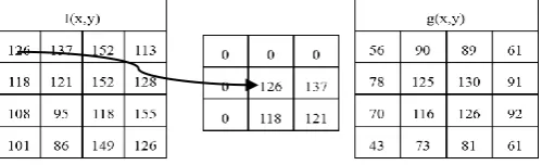
(9) For example let us take an image of size 4*4 as shown in figure 1 (a) and its average intensity g(x,y) is calculated by padding required number of zeros at edges as shown in figure 1 (b). First table in figure is image and first element i.e 126,

g(x,y) is calculated by padding zero’s at edges as in figure and last tables shows g(x,y) for entire image I(x,y). 2-D histogram of Lena image at marked area is shown in figure 2, where diagonal quadrants carry much information.

The 2-D histogram of tested images as shown in figure 2 and are divided into four clusters by a single threshold (t,s). Where t is threshold for original image intensity I(x,y) and s is threshold for average intensity image g(x,y). The divided cluster area is not same. The diagonal quadrant 1st represents object and 3rd represent background and 2nd and 4th quadrants are neglected because does not carry any information (pair occurrence is less) as show in figure. The Renyi entropy for object and background is given as

(10)

(11)

Where and

The final objective function which is to maximized for better threshold (t,s) selection is

(12)

2.2 Proposed Renyi 2d-Hisotgram Based Multi-Level Thresholding

International Journal of Innovative Technology and Exploring Engineering (IJITEE) ISSN: 2278-3075, Volume-8 Issue-10, August 2019

( a )

( b )

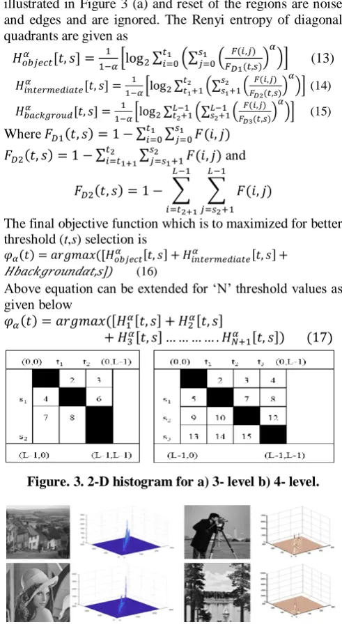
In this paper, we proposed a 2-D Renyi entropy based multilevel thresholding for image segmentation by incorporating the advantage of 2-D histogram. If the 2-D histogram of an image is cluster into 9 clusters with two thresholds (t1, t2) and (s1, s2) as shown in figure 3 (a). Then the diagonal quadrants 1st, 5th and 9th represents objects(s), intermediate regions and background respectively as illustrated in Figure 3 (a) and reset of the regions are noise and edges and are ignored. The Renyi entropy of diagonal quadrants are given as

(13)

(14)

(15)

Where

and

The final objective function which is to maximized for better threshold (t,s) selection is

, ]) (16)

Above equation can be extended for ‘N’ threshold values as given below

Figure. 3. 2-D histogram for a) 3- level b) 4- level.

Figure. 4. Input images and corresponding 2-D histogram

Where

(18)

For simplifying the calculations, two dummy thresholds are introduced t0 and tN+1= L-1 which satisfy the condition t0 < t1………. < tN-1< tN+1. Similarly two dummy variable s0 and sN+1 = L-1 which satisfy the condition s0 < s1………. < sN-1< sN+1. The 2-D histogram of four standard images are shown in figure 4 and form these figure it is observed that most of the information/energy is concentrated on diagonal quadrants. Multilevel thresholding is a time consuming process and is proportional to the number of thresholds ‘N’. So soft computing techniques play a significant role in this contest by assuming eqn. (17) as an objection function, which leads to reduction in the computational time.

III. PROPOSED HBFOA-PSO

This paper mainly focuses on optimization of thresholds levels for optimal image segmentation. An attempt is made on the basis of hybridizing the two well-known metharustic optimization techniques such as particle swam optimization (PSO) and bacterial foraging optimization algorithm (BFOA). The BFOA being a global search algorithm it found many applications in the field of engineering and medical applications and sometimes it may follow into local optimal solution. To avoid the limitations of BFOA, a PSO algorithm is introduced which speedup the execution time and avoids being follow in local optimal solution. The hybridized algorithm is called hBFOA-PSO which is further used for optimal thresholding for effective image segmentation and obtained evaluations are compared with state of art optimization algorithms. In the following section all the algorithms are explained clearly in all accepts.

3.1 Bacteria Foraging Optimization Technique: Overview

The scientist named Passino introduced BFOA in 2002 and is algorithm is developed based on in depth study on behaviour of Bacteria in process of foraging for food in any substances [15]. The bacteria named E.Coligains energy by searching for nutrients per every minute. This nutrients search may be occurred by sharing information among the bacteria’s. Another way of getting nutrients is by following three steps: swarming or tumbling and chemotaxis step. In algorithm structure of BFOA, search process is extraordinary because of its inbuilt well established algorithm follow. In searching process of food, BFOA follows a step size based on Gaussian distribution function, whereas cuckoo search following Levydistribution. The optimal thresholds are acquired by optimizing the Renyi’s entropy in two dimensional with BFOA. The algorithm directs all bacteria’s towards maximizing the Renyi’s entropy fitness function. Initially all the bacteria’s are randomly selected so each one carries different objective values and in every iterations these values are updated by learning themselves. The highest objective function holding bacteria is forwarded to next iterations and least bacteria are replaced with new ones. In each iterations rest all bacteria’s try to follow the highest objective bacteria. This process is repeated until the required objective function value achieved. The BFOA achieve this optimal result in four poured stages: 1. Chemotaxis, 2.Reproduction 3.Elimination-dispersal 4.swarming. These four stages of BFOA are explained below.

Counter clockwise rotation

TUMBLE

Figure 5.Bacterium tumbling stage

SWIM

Clockwise rotation

Tumbling: In this stage bacteria move arbitrarily in a certain direction where extraordinary nutrients are existing in search space. All the bacteria have initially some nutrients naturally. This procedure is identified as tumbling process as shown in Figure 5.

Swimming (up): Nutrient obtained after tumbling, if those are sufficient and successful then bacteria move in same path in order to increase further or else it go for swimming process. This movement of swimming is called swimming up.

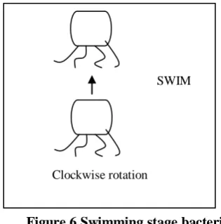
Swimming (down): If bacteria moving path decrease the bacteria nutrients then that movement sare known as swimming down. When bacteria finds swimming down stage then instantly bacteria change its path. Figure 6 shows swimming stage.

Figure 6.Swimming stage bacteria

The bacteria step of chemo tactic is given in Eq. (19).

(19)

Where C(x) is bacteria step size and Δ (x) is randomly chosen floating number between [0,1].

2. Swarming: In this stage bacterium tires to communicate with each other for better improve of their positions towards getting better and high quality nutrients for better survival or to extend their life span. So remaining bacteria always try to moves toward highest nutrients bacteria direction and circumvents the path of movement toward the lowest nutrient. This process usually called swarming and below equation described this step.

3. Reproduction: Before applying this step on bacteria, all the bacteria are assigned ranked based on fitness value either in descending or ascending order depends on maximization or minimization problem respectively. As entropy must to be maximum so in this paper all the bacteria’s are ordered in ascending order as per their objective values. In this stage half of the bacteria’s with lowest ranks are died and are replaced with the new generation generated by mutation between two largest objective value bacteria’s. So that number of populations or solutions sin search space is same. This entire process is called conjugation.

4. Elimination-dispersal: In some situations bacteria may familiarity an unexpected change in eco friendly situations like hike in humidity or in temperature. Then bacteria experiences third stage i.e. reproduction, in which bacteria dies because of unexpected changes and new bacteria’s are produced by a sexual relative between two other bacteria. Some bacteria’s may be moved to the nearest and safest place.

BFOA Algorithm: For i = 1:Med For j = 1:Mre For k = 1:Mc For l = 1:SU

J(i,j,k,l) = J(i,j,k,l)+Jcc[

Calculate the J (i,j+1,k,l)

p = 0; While p<Ml MM = M+1 If J (i,j,k,l) <

update Jlast1

else mmm = Ms

End if End while End j End k End l For i =1:SS

=

International Journal of Innovative Technology and Exploring Engineering (IJITEE) ISSN: 2278-3075, Volume-8 Issue-10, August 2019

End j For i = 1:SSS If randn () <Pedd

Unhealthy bacteria will be eliminated and swap with a new randomly produced

End if End p End l

3.2 Particle Swarm Optimization (PSO)

Kennedy and Eberhart proposed a new optimization i.e PSO in 1995. The PSO is a stochastic methodology under swarm based intelligence and it mimics in what way particle is moving to get best food for survival [16]. Every particle individually and adaptively updates the position and velocity around the search space based on the experience of previously obtained knowledge around its space and the understandings of additional particle in the populations. Every particle is given with a temporary memory by which particle store the good food location it forever visited during its expedition. Particle good food location is treated as Pbest and the best good location of group occupied as one is stowed as Gbest. The preliminary positions of Pbest and Gbest are dissimilar. Particle is showed to give the better results in procurement the global maxima or minima. However, getting the global minima/maxima optimum value is a stimulating matter, whenever there will be multiple minima happens. This PSO algorithm doesn’t involve mutation or crossover operators. It depends on initialization of the tuning parameters, the swarm size, the objective/fitness function and the minima/maxima number of iteration. It doesn’t depend on the preliminary conditions and the incline values.

The compensations of using the PSO are less expensive in computationally, abundant simple to instrument, Lower CPU time and requirement of memory[19]. The each particle modified velocity is given in Eq (21)

(21)

The each particle position modified with below equation

(22) Algorithm of PSO:

Step 1: Initialize every individual particle in solutions with randomly position & randomly velocity.

Step 2: Calculate the objective/cost function of every particle. If the present objective/cost is sophisticated than the finest value up to now calculated, then it is stowed in Pbest. Step 3: Find the highest objective/cost particles among all and assume that position is Gbest.

Step 4: Find the fresh velocity and position of every particle rendering to the above equations.

Step 5: Reiteration the above all steps from 2-4 till maximum iterations or minimum/maximum criteria.

3.3 hBFOA–PSO ALGORITHM

The hBFOA–PSO syndicates PSO and BFOA algorithms, so it earnings the disadvantages and advantages of both algorithms. The goal is to share/support information among BFOA and PSO that pointers to generation of healthy and wealthy bacteria by means of elimination and dispersal. The main disadvantage in BFOA is, tumbling step is random in all iterations, so attaining a global solution/result is difficult. Whereas, in proposed hybrid BFOA-PSO algorithm, the tumbling step is not random in every iterations and with the help of PSO these steps of tumbling is optimized. The suitable& better tumbling step and global best

result from PSO is prearranged as input to the BFOA. Tumbling steps are updated at first step of BFOA. The parameter notations for hybrid BFOA and PSO given is below.

Step 1: parameters Initialization for both PSO and BFOA: pp = Problem dimensions;

SS = population/solutions size or in case of PSO number of particle and number of bacteria in case of BFOA;

NNs = length of swim in chemotaxis loop, followed by tumbling stage;

NNc = stopping criteria or iterations maximum NNre = Max reproduction step;

NNed = Max number of steps in case of elimination and dispersal;

PPed = probability of dispersal and elimination

CC(i) =tumbling step size; , , , = Bacteria

repellent and attractive coefficients;

Δ (pp, ii) = Bacteria’s direction in present iteration; P (ii, jj) = Bacteria’s position in present iteration;

, = PSO tuning parameters;

r1, r2 = randomly selected numbers [0 to 1] in PSO; Step 2: dispersal and Elimination loop: ss = ss + 1. Step 3: Reproduction loop: rr = rr + 1.

Step 4: Chemotaxis loop: qq = qq + 1.

Sub step aa: For pp = 1, 2, . . . , SS, ith bacteria’s moves with following steps

 Find all bacteria’s objective/fitness value, Jj(i,j,k,l); henceforth new fitness/objective function is Jj(i,j,k,l) = - Jj(i,j,k,l) + Jccc (hh (j,k,l), Pp(j,k,l));

 Assign Jj_last = Jj (j,k,l).

Sub step bb: For pp = 1, 2, . . . , SS bacteria’s categorical to take either swimming or tumbling Δ(ii), that is random generation lies numbers0 to 1between in first iterations for all bacteria’s or for all solutions/populations. From second onwards iterations tumbling and directions are optimized with the help of PSO. Bacteria’s move towards best direction with

Where j, k and l are indexes of Chemotaxis steps, re-production and Elimination & dispersal respectively. Which leads pthbacteria will move with a step size of Cc(i) in tumbling stage

Calculate J (i,j,k,l)=J(i,j,k,l)+Jccc[

 Stage: Swimming

i. Assume mm = 0 (hostage for swim length). ii. While mmm<NNs

Let mmm= mmm + 1

If J(i,j+1,k,l) < , let = |J(i,j+1,k,l)| and

1,r,s= j,k,l+ . ( ) ( )

Sub-step c: If pp SSs Next bacteria (j + 1) (i.e., go to sub-step b for next bacteria)

Step 5: calculate global and local best positions of each bacteria’s.

Step 6: updated every bacteria’s velocity and position with PSO. New update vector (pp, p).

Step 7: If j<NNc, go to stage 4 and repeats chemotxis step until the bacteria’s alive.

 Sub-step a: Find fitness of bacterium p by significant the s and r value, as

. show the

amount of nutrients a bacteria has over its total generation and it’s a quantity of success of bacterium in circumventing noxious materials. As per the values,

Category all bacterium in rising order and also chemotactic parameter C (p).

 Sub-step bb: The SSr = SSS/2, the uppermost values of

bacteria are uninvolved and rest Sr bacterium with the finest value divided. New bacteria are placed at the

same location.

Step 9: If ss<NNre, moves to step 3.

Step 10: dispersal and Elimination: For j = 1, 2. . . SSS, with probability , eliminates and disperses each bacteria.

IV. RESULTS AND DISCUSSION

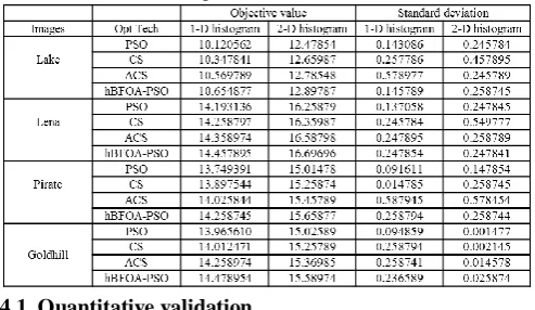
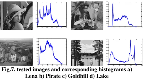
The proposed algorithm performance is evaluated by considering the standard benchmark images like Lena, Goldhill, Lake and pirate and all the images are of size 256×256 and each pixels take 8 bits (bits per pixel = 8). All the images are in ‘.tif’ format except Lake which is in .gif and Goldhill is in .jpeg format as shown figure 7. All the algorithms are simulated in Mat lab version 2017 and implemented in desktop with specifications: Windows 7 Enterprise N, HP Compaq LE1902x, Intel (R) Core (TM) Duo CPU e7500N at 2.93GHz, 64-bit operating system. The number of iterations itr = 50, population size P = 100, upper bound Ub= 255, Lb= 0, dimensions of the problem D = th are consider for all optimization algorithms. In this paper, number of thresholds t = 5 selected for all algorithms because the number of thresholds in published previous paper is 5. The proposed approach is tested by thresholding the image with the help of both 1-D histogram and 2-D histogram and compared the results with the ACS, PSO and CS. The same tuning parameters as in [17] are taken for CS and PSO. Table 1: Comparison of Objective Value & Standard deviation for various algorithms.

4.1. Quantitative validation

To inspect the influence of the hBFOA-PSO algorithm for the problem of multilevel thresholding, we considered Renyi entropy as objective function or fitness function. The Hybrid Bacterial Foraging Optimization Algorithm and particle swarm optimization and other three algorithms are applied on Renyi entropy objective function and the results of the hBFOA-PSO are compared with ACS, PSO and CS in both 1-D and 2-D histogram. To maximize the objective function all the algorithms are optimized. Table 1 shows the objective function for hBFOA-PSO, ACS, PSO and CS. Hence from Table. 1 by using Renyi entropy the objective value obtained with 2-D histogram for different images are higher than with 1-D histogram and proposed

hBFOA-PSO objective value is higher than ACS, PSO and CS with both histograms.

4.2 Peak Signal to Noise Ratio and Mean Square Error

The PSNR illustrates the variations among the threshold image and input image. In general the measure of visual difference of two images and units are decibels (dB). If the reconstructed image shows the better quality, it indicates the higher value of PSNR.

The below equation (23) to calculate Peak signal to noise ratio value, is output vector and is input vector shown below.

(23)

The below equation (24) to calculate Mean square Error value, Y is output image and X is input image and M x N is the size of image shown below.

MSE =

(24)

The values attained for the PSNR from the different algorithms are shown in Table 2, when compared to ACS, PSO and CS, the proposed algorithm attains higher PSNR value with 2-D histogram as compared to 1-D histogram. So the quality of the reconstructed images gets much better for the higher level of thresholds. Also, results displayed in table 2, suggest that A 2-D Histogram on the image set produce a much better PSNR than the 1-D histogram and quality of images reconstructed from the 2-D histogram fare much better than its 1-D counterpart. The mean square error between the reconstructed and original image is less for hBFOA-PSO compared to other methods as tabulated in Table 2.

4.3. Misclassification error:

It shows the segment numbers which are misclassified in between the original images and segmented images. Assume one pixel actually is in foreground but unfortunately treated as background pixel then we treat that pixel is misclassified. In similarly, a collection of pixels comes underneath background but those are treated as foreground then the resultant segmentation is misclassified and is calculated by below Eq. 25

2 0

2

max min

(I )

1 2

(I I )

j Th

i j

j i R

M t

N



 

    

 

 

(25)

International Journal of Innovative Technology and Exploring Engineering (IJITEE) ISSN: 2278-3075, Volume-8 Issue-10, August 2019

0 50 100 150 200 250 300 0

100 200 300 400 500 600 700 800 900 0 50 100 150 200 250 300

0 100 200 300 400 500 600

0 50 100 150 200 250 300 0

100 200 300 400 500 600 700 800 900 1000

0 50 100 150 200 250 300 0

50 100 150 200 250 300 350 400 450

Fig.7. tested images and corresponding histograms a) Lena b) Pirate c) Goldhill d) Lake

Where tis number of required segment regions or dimensions of thresholds,Rjis jth segment regions, pixel intensity levels are Iiat definite segment region, σjis jthmean of all segment regions, image size is N(number of rows * column), Imin is lower intensity of input image (between 0 in case of gray scale image and three for color) and Imax higher intensity level of an image (255 in case of gray scale). Many times, misclassification error does layin-between 0 to 1 and lower value of misclassification value shows to best image segmentation and highest misclassification shows nastiest segmentation. Henceforth, the misclassification error, in segmentation is measure of difference in-between maximum 1 (better quality in visual) and minimum i.e 0 (not good quality in image). A comparison of the hBFoA-PSO with respect to the other models is made and the Misclassification error and SSI are displayed in Table. 3. The results ascertain that our proposed model performs better with a lowest error and better segmentation is achieved when used in combination with a 2-D histogram than 1-D histogram. Table 3: Misclassification error & Structural Similarity Index

4.4. Structural Similarity Index (SSIM)

It guesses the visual resemblance in between input and segmented/threshold image and is measured from Eq. (26)

2 2 2 2

(2

C1)(2

C2)

(

C1)(

C2)

I I II

I I I I

SSIM

 



 

 







_{ }

_{ }

Where µI and µĨ are the mean of input I and segmented Ĩ image, σI and σĨ are the standard deviation of input I and segmented Ĩ, σIĨ is cross correlation and C1 and C2 are fixed values and is 0.065 in this work. Table. 3 demonstrate the SSIM for various techniques along Renyi entropy and it reveal proposed higher SSIM with 2-D histogram as compared to 1-D histogram and is higher than other methods too.

4.5. Qualitative Results

Here we focused on visual clarity of reconstructed image which are obtained by thresholding the image in both 1-D histogram and proposed 2-D histogram by maximizing the Renyi entropy with proposed hybrid BFOA-PSO and with ACS, PSO and CS. The segmented images and histogram

obtained with 1-D histogram and proposed 2-D histogram with hybrid BFOA-PSO algorithms at threshold level 5 with Renyi entropy are shown in Figure 8. As we know, at higher levels of threshold (i.e, (t = 5) compared to t = 2, t = 3 and t = 4) the constructed image visual quality is much better. For efficiency measure of proposed Hybrid BFOA-PSO, let us have a look at the visual quality of few segmented images with Renyi entropy: Pirate image at 5 level thresholds as in Figure. 8b, Lena image at 5 level thresholds as in Fig. 7a from these figures h BFOA-PSO segmented visual quality is better with 2-D histogram as compare to 1-D histogram. Similarly, for Renyi entropy segmented visual quality of proposed hBFOA-PSO is better with 2-D histogram. For example, Goldhill image at 5 level thresholds as shown in Fig.8c and Lake image at 5- level thresholds as shown in Fig.8d. When comparing the quality of an image, the proposed algorithm performs better than the existing approaches. In Fig. 8d, Visibility of the background lake is poor with 1-D histogram at five level thresholds. But it is clearly visible with 2-D histogram. Moreover as the number of thresholds is increased the images becomes clearly recognizable.

Figure 8. Segmented images with 1-D and 2-D histogram respectively a) Lena b) Pirate c) Goldhill d) Lake

V. CONCLUSIONS

Author-2 Photo

Author-3 Photo

REFERENCES

1. De Luca. A, S. Termini, A definition of non-probabilistic entropy in the setting of fuzzy sets theory, Inf. Control 20 (1972) 301–312.

2. Sezgin. M, B. Sankur, Survey over image thresholding techniques and quantitative performance evaluation, J. Electron. Imaging 13 (1) (2004) 146–165.

3. Kapur. J. N, P.K.Sahoo, A.K.C Wong, A new method for gray-level picture thresholding using the entropy of the histogram”, Computer Vision Graphics Image Process. 29 (1985) 273 – 285.

4. Otsu. N, “A threshold selection from gray level histograms” IEEE Transactions on System, Man and Cybernetics 66, 1979.

5. Sathya. P. D and R. Kayalvizhi, “Optimal multilevel thresholding using bacterial foraging algorithm”, Expert Systems with Applications, Vol. 38, pp. 15549–15564, 2011.

6. Mbuyamba. M, J. Cruz-Duarte , J. Avina-Cervantes, C. Correa-Cely, D. Lindner, and C. Chalopin, “Active contours driven by Cuckoo Search strategy for brain tumour images segmentation”, Expert Systems With Applications, Vol. 56, pp. 59–68, 2016.

7. Ye. Z, M. Wang, W. Liu, S. Chen, “Fuzzy entropy based optimal thresholding using bat algorithm”, Applied Soft Computing, Vol. 31, pp. 381–395, 2015.

8. Agrawal. S, R. Panda, S. Bhuyan, B.K. Panigrahi, “Tsallis entropy based optimal multilevel thresholding using cuckoo search algorithm”, Swarm and Evolutionary Computation, Vol. 11 pp. 16–30, 2013.

9. Horng. M and T. Jiang, “Multilevel Image Thresholding Selection based on the Firefly Algorithm”, Symposia and Workshops on Ubiquitous, Autonomic and Trusted Computing, pp. 58–63, 2010.

10.Bhandari. A. K, A. Kumar, G. K. Singh, "Tsallis entropy based multilevel thresholding for colored satellite image segmentation using evolutionary algorithms”, Expert Systems With Applications, Vol. 42, pp. 8707–8730, 2015.

11.Naidu. M.S.R, Rajesh Kumar. P, “Tsallis Entropy Based Image Thresholding for Image Segmentation”, Computational Intelligence in Data Mining, Vol. 556, pp 371-379, 2017.

12.Naidu. M.S.R, Rajesh Kumar. P, Karri. C, “Shannon and Fuzzy Entropy based Evolutionary Image Thresholding for Image Segmentation” Alexandria Engineering Journal, doi.org/10.1016/j.aej.2017.05.024, 2017.

13.Rényi, A, “On measures of information and entropy”, In Proceedings of the 4th Berkeley symposium on mathematics, statistics and probability, pp.547–561, 1960.

14.Soham S and Swagatam Das, “Multilevel Image Thresholding Based on 2D Histogram and Maximum Tsallis Entropy A Differential Evolution Approach”, IEEE Transactions On Image Processing, Vol. 22, No. 12, pp. 4788, 2013.

15.Passino KM (2002). Biomimicry of bacterial foraging for distributed optimization and control, IEEE Control Systems Magazine, 22: 52–67. 16.Kennedy J, Eberhart RC (1995). A new Optimizer using Particle Swarm

Theory, in Proceedings of Sixth International Symposium on Micro Machine and Human Science, Nagoya, Japan, 6: 39-43.

17.Karri. C and Jena. UR, “Hybrid gravitational search and pattern search–based image thresholding by optimizing Shannon and fuzzy entropy for image compression”, International Journal of Image and Data Fusion, Vol. 8, No. 3, 2017.

18.Rényi, A, “On measures of information and entropy”, In Proceedings of the 4th Berkeley symposium on mathematics, statistics and probability, pp.547–561, 1960.

19.Kumar N.S.R., Phanindra & Reddy P.V.G.D., Prasad. (2019). Evolutionary Image Thresholding for Image Segmentation. International Journal of Computer Vision and Image Processing. 9. 17-34. 10.4018/IJCVIP.2019010102.

AUTHORSPROFILE

N S R Phanindra Kumarobtained his B Tech (CSE)

from JNTU, Kakinada in 2010 and M Tech in computer science & Engineering from AU college of engineering, Vishakhapatnam in 2013. He is working as an assistant professor in the Department of CSE, AITAM, tekkali, Srikakulam. His areas of interest include image processing and soft computing techniques.

Prof. Prasad Reddy, P.V.G.D, obtained his B.Tech, in

Mechanical Engineering, from Andhra University and M.Tech, in Computer Science & Technology, and Ph.D, in Computer Engineering. He is presently the SeniorProfessor in Computer Science & Systems

Engineering department. He has to his credit, more than 120 Research papers which includes around 95 publications in the referred indexed Journals. His Research areas include Soft Computing, Software Architectures, knowledge Discovery from Databases, Image Processing, Number theory &Cryptosystems. He has 24 years of teaching & research experience which includes more than 10 years of administrative experience with Andhra University at various senior capacities..

Dr G.Srinivas obtained his M.Tech, in Computer