Voltage Slump Compensation using Facts Controllers on Power System

(1)



Abstract: This article dispense the different FACTS controllers

integrated circuits using a simulation program that emphasis

with PSPICE. The FACTS controller controls series impedance,

shunt impedance, voltage, current and phase angle. In this paper, a simplified circuit model of Series Compensator and Unified Power Quality conditioner has been analyzed and the simulation results coincides with the theoretical results..

Index Terms: FACTS controllers, FACTS, power electronic

equipment, Compensator, UPQC.

I. INTRODUCTION

At the present time, the active methods for power quality control have become more appealing correlate with passive ones due to their compact size, fast response, and higher performance. The state estimation algorithm has been proposed related to the performance with the IEEE standard system, that has been modified by the inclusion of UPQC. As a result, observing and checking these FACTS devices and their respective parameters is also being to be pivotal for power system control. Various devices on FACTS are thyristor controlled series compensation (TCSC) and unified power quality controller (UPQC) [1]. A UPQC be composed of shunt and series voltage converters in contact to a transmission line that permits the individualistic control of the real and the reactive power flows through the line [2, 3]. In order to determine the condition for the power system FACTS devices, a better forming method to separate the power network, TCSC and UPQC, thereby permitting a forming solution, being proposed [4]. Nevertheless, the limitations of these devices are not contemplated. The UPFC’s limitations are, the condition approximation problem gets the nonlinear weighted least squares (WLS) optimization with a set of equality and inequality limitations [5]. Then this optimized solution obtained by employing a solution method based on the interior point method [6].

The weighted least absolute value condition approximation has been far apart used for power system condition approximation [7]. In spite of, providing a quick retaliation, it is not vigorous in the existence of the bad computation. A special standard called the WLAV can be employed to enhance the efficiency [8]. The Weighted least

Revised Manuscript Received on September2, 2019.

S. Sankar, Professor, Department of EEE. Sriram Engineering College,

Chennai, TN, India

M. N. Saravana Kumar, Assistant Professor, Department of EIE. Erode

Sengunthar Engineering College, Erode, TN, India.

P. Prabhu, Associate Professor, Department of Mechanical Engineering. Sriram Engineering College, Chennai, TN, India.

Dr. D. Sivanandakumar, Assistant Professor, Electrical and Electronics Engineering,

absolute value (WLAV) is able to refuse the bad computation as long as these are no dominance points [9, 10]. Lately, the appeal of the interior point method for WLAV condition approximation of the standard power system has been dispensed [11, 12].

In this paper, we suggested a technique for resolving the condition approximation problem accommodating UPQC by contrive the difficulty as a nonlinear WLAV makes the best, with a set of equality and inequality nonlinear constraints.

II. SERIESCOMPENSATOR

A. Review Stage

A series compensator circuit is shown in Fig.1 that incorporates two capacitors connected in series with the line. The resistance in series with the capacitor is the current limiting resistance. The AC switches are connected in parallel with the respective capacitors.

1 2

[image:1.595.316.543.400.536.2]

0

Fig. 1. Series Compensator

The simulated waveform in Fig. 2 represents at Inductor alone and with switch to be in closed state.

T i m e

1 5 0 m s 2 0 0 m s 2 5 0 m s 3 0 0 m s 3 5 0 m s 4 0 0 m s 4 5 0 m s 5 0 0 m s 5 5 0 m s

1 0 1 m s 6 0 0 m s

W ( R 1 ) 0 W 4 0 K W 8 0 K W 1 2 0 K W 1 6 0 K W 2 0 0 K W

Fig .2. Power waveform (195 kw)

Voltage Slump Compensation using Facts

Controllers on Power System

[image:1.595.318.544.577.699.2]

(2)

The simulated waveform in Fig. 3 represents at Inductor and capacitor and with switch to be in open state.

Time

420ms 440ms 460ms 480ms 500ms 520ms 540ms 560ms 580ms

405ms 600ms

[image:2.595.311.543.50.196.2]

W(R1) 0W 200KW 400KW

Fig .3 Power waveform (400kw)

It has been analyzed from Fig. 2, when inductor alone is added, the power transmitted is 195 KW. As the same, shown in Fig. 3, on adding a capacitor to the system, the power transmission can be increased to 400 kW.

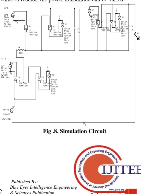
III. SERIESCOMPENSATORWITHCAPACITORS If The simulation circuit with two capacitors and one uncontrolled reactor is shown in Fig. 4.

R3 100 C4

25u

+

-+-S4

S VON = 1.0V VOFF = 0.0V

C3 25u

V6

TD = 10 TF = 1n PW = 18m PER = 20m V1 = 0 TR = 1n V2 = 5

L2

1000m

1 2

W

0 -+

+

- S7

0 _V5

TD = 10 TF = 1n PW = 18m PER = 20m V1 = 0 TR = 1n V2 = 5 0

0 V4

TD = 1

TF = 1n PW = 18m PER = 20m V1 = 0

TR = 1n V2 = 5

V7

TD = 1 TF = 1n PW = 18m PER = 20m V1 = 0 TR = 1n V2 = 5

+

-+

- S6

0

V8

FREQ = 50 VAMPL = 230 VOFF = 0

+

-+ -_S5

[image:2.595.61.292.82.208.2]

Fig.4 Simulation Circuit with two capacitors and one uncontrolled reactor

By introducing the capacitor in the system, the power transmitted can be increased. As shown in the Fig. 5, that inductor alone is present in the system; the power transmitted is 47 Watts. As shown in the Fig. 6, when one capacitor is introduced into the system, the power transmitted increases to 110Watts. As shown in the Fig. 7, when two capacitors are introduced into the system, the power transmitted increases to 345Watts.

Time

30ms 40ms 50ms 60ms 70ms 80ms 90ms 100ms

W(R3) 0W 20.0W 40.0W 50.5W

Fig. 5. Power waveform with inductor alone.

Time

40.0ms 50.0ms 60.0ms 70.0ms 80.0ms 90.0ms

[image:2.595.310.545.205.341.2]

36.1ms 100.0ms W(R3) 0W 50W 100W 121W

Fig.6. Power waveform with inductor and one capacitor

Time

45.0ms 50.0ms 55.0ms 60.0ms 65.0ms 70.0ms 75.0ms 80.0ms 85.0ms 90.0ms 95.0ms

[image:2.595.49.292.350.527.2]

40.4ms 100.0ms W(R3) 0W 100W 200W 300W 400W

Fig .7. Power with inductor and two capacitors with both switch open

IV. SERIES COMPENSATOR WITH TWO CAPACIT

ORS AND SINGLE UNCONTROLLEDREACTOR

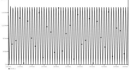
By varying the reactor connection in the system, the power transmitted can be varied. The simulation circuit is shown in the Fig. 8. As shown in the Fig.9, when a reactor is introduced into the system at a firing angle delay of 90°, the power transmitted is 110 KW. As shown in the Fig.11, when a reactor is introduced into the system at a firing angle delay of 63°, the power transmitted is 260 KW. Thus by varying the value of reactor, the power transmitted can be varied.

C3 25u

+

-+-S5

S VON = 1.0V VOFF = 0.0V V6 TD = 10m TF = 1n PW = 18m PER = 20m V1 = 0 TR = 1n V2 = 5

C4 25u

V10 TD = 15m TF = 1n PW = 10m PER = 20m V1 = 0 TR = 1n V2 = 5

0

+

-+-S4

V8 FREQ = 50 VAMPL = 11k VOFF = 0

V9 TD = 5m

TF = 1n PW = 10m PER = 20m V1 = 0

TR = 1n V2 = 5

W

0

+

-+-S9

+

-+

- S6

S VON = 1.0V VOFF = 0.0V V4

TD = 0m TF = 1n PW = 18m PER = 20m V1 = 0

TR = 1n V2 = 5

R3 100 0 L4 1000m 1 2

0 -+

+

- S7

0 0 0 + -+ - S8 S VON = 1.0V VOFF = 0.0V

[image:2.595.304.545.500.830.2] [image:2.595.53.290.642.765.2]

(3)

The waveform of series compensator with inductor alone is shown in Fig .9.

Time

0s 10ms 20ms 30ms 40ms 50ms 60ms 70ms 80ms 90ms 100ms W(R3)

[image:3.595.322.544.52.379.2]

0W 50KW 100KW 150KW

Fig.9. Power waveform of series compensators single controlled reactor

The waveform with inductor and one capacitor is shown in Fig .10.

Time

40.0ms 50.0ms 60.0ms 70.0ms 80.0ms 90.0ms

35.3ms 100.0ms

W(R3) 0W 100KW 200KW 300KW

Fig.10. Power waveform of series compensator with one inductor and one capacitor

V. PERFORMANCEOFUPFCANDUPQC

On Consider a simple two-machine transmission model as shown above, the source of variable phase angle is inserted at the midpoint of a model. Mid point is the best location because, the voltage drops along the not compensated transmission line is the extensive at the midpoint. The compensation at mid point, shatters the transmission line into two equal divisions for each of which transmittable power is the same. By changing the phase angle of midpoint source, the real power transmitted can be varied. When the phase angle of midpoint source is set at 60˚ and 270˚, the corresponding variation in real power is shown in the results below. Thus on managing the phase angle of midpoint source, the flow of real power can be managed. The simulation circuit of UPFC is as shown in the Fig.11.

V2

FREQ = 50 VAMPL = 11k VOFF = 0

V1

FREQ = 50 VAMPL = 2000 VOFF = 0 L1

60m

1 2

R2 2 V+ L2

60m

1 2

R1 0.001

TX1

TN33_20_11_2P90

0

V+

V-0

Fig .11. Simulation Circuit of UPFC

Time

0s 50ms 100ms 150ms 200ms 250ms 300ms 350ms 400ms

V(L1:1,0) -20KV

0V 20KV

SEL>> V(L2:2,0) -1.0KV

0V 1.0KV 2.0KV

Fig. 11(a) For an angle of injection at 60o Sending and receiving End voltages

Time

250ms 300ms 350ms 400ms 450ms 500ms 550ms

201ms 600ms

W(R2) W(R2) 0W

100KW 200KW

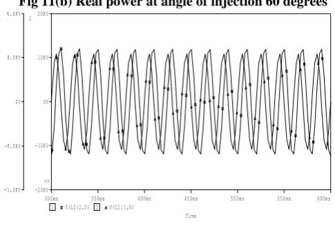
Fig 11(b) Real power at angle of injection 60 degrees

Time

300ms 350ms 400ms 450ms 500ms 550ms 600ms

1 V(L2:2,0) 2 V(L1:1,0) -1.0KV

-0.5KV 0V 0.5KV 1.0KV 1

-20KV -10KV 0V 10KV 20KV 2

>>

[image:3.595.76.277.74.199.2] [image:3.595.67.279.262.409.2] [image:3.595.306.549.545.709.2]

(4)

Time

320ms 360ms 400ms 440ms 480ms 520ms 560ms

299ms 600ms

W(R2) 50KW 100KW 150KW

9KW

Fig. 12(b) Real power at angle of injection 270 degrees

The above results clearly shows that the real power flows for 60° is 160kw and real power flow can be controlled on increasing the injecting angle. The angle of injection for 270°. The real power flow will be decreased by 135kw. In this analysis it has been observed that, the transmitted power can be varied by changing the angle of injection. In the Fig. 13 depicts the amended IEEE 14-bus system. One UPQC is located in branch 6-12 at bus number 6. Table I shows the variables and limitations of the UPQC. The computed data's are given in Table II. The computed set inheres of 32 flow measurement, 12 power injections, and 2 voltages. Note that the computation set will create the network and UPQC fully perceptible. The reckon states of the UPQC are recaptitulate in Table III. It is observed that the UPQC conditional approximation and its apparent powers are inside its boundary. The real power shift between both voltage sources is close to zero, Psh + Pse = 0.

[image:4.595.69.271.53.183.2]

The simulation diagram of the proposed method of UPQC is shown in the figure 13. The three phase source volt age is shown in the figure 14.

Fig.13 Simulation Diagram for Proposed Method of UPQC

Fig.14. Waveform of Line Voltage

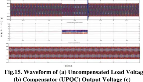
Here in this system, there is no compensator; the load voltage gets reduced due to the addition of non-linear loads. In the Fig. 15 (a) shows the decrease in voltage due to the

[image:4.595.308.543.139.274.2]

addition of non-linear load. It can be observed that there is a decrease in voltage at the interval of 2 to 3 cycles. By performing the output of Figure 15 (b) shows the output voltage of the compensator. It provides the voltage only in the interval of 2 to 3 cycles. Figure 15 (c) shows the compensated load voltage. In this we can see the rated voltage is obtained at the receiving end of the power system.

Fig.15. Waveform of (a) Uncompensated Load Voltage (b) Compensator (UPQC) Output Voltage (c)

Compensated Load Voltage

[image:4.595.309.542.419.679.2]

The voltage across DC link capacitor is shown in the Fig 16. From this we can depict that the magnitude of voltage is between 0 to 22V. When compared to conventional method the value of DC link voltage obtained is less. So the level of the harmonic imbalance in the injected voltage will be reduced. Hence by this method the harmonics present in the load voltage will be considerably reduced and the power quality of the same will be improved. The Fig.17 gives the percentage of the Total Harmonic Distortion (THD) obtained by this proposed method.

Fig.16 Waveform of DC Link Capacitor Voltage for proposed method

[image:4.595.53.282.469.743.2]

(5)

[image:5.595.59.277.142.310.2]

From the Fig.17 we can depict that the percentage of Total Harmonic Distortion (THD) is 0.21%. Thus the harmonic content in the load voltage is reduced. When compared to the conventional method, total harmonic distortion (THD) is limited in our suggested model. Also the power factor is improved. The IEEE 14-bus system with UPQC is as shown in the Fig.18.

Fig. 18. IEEE 14-bus system with UPQC.

Table I: Variables and limitations of UPQC in IEEE 14-Bus System

Shunt Source Series Source

Rsh 0.00 Rse 0.00

Xsh 0.05 Xse 0.05

Vsh,max 1.11 Vse,max 0.59

Ssh,max 0.11 Sse,max 0.09

Table II: Computed Data's of IEEE 14-Bus System Bus voltage measurements

Bus Voltage Bus Voltage

1 1.06 4 1.012

Injection measurements

Bus P Q Bus P Q

3 -0.8419 0.0432 8 -0.0011 0.17

9 -0.295 -0.166 10 -0.09 -0.06

13 -0.132 -0.06 14 -0.15 -0.1

Flow measurements

Branch P Q Branch P Q

1-5 0.8591 0.04 2-3 0.8 0.034

2-5 0.42 0.001 4-7 0.3 -0.1

4-9 0.16 -0.01 6-5 -0.5 -0.13

6-11 0.063 0.04 6-12 0.3 0.013

7-9 0.28 0.11 8-7 -0.0019 0.23

9-7 -0.281 -0.05 9-14 0.1 0.034

10-11 -0.03 -0.02 12-6 -0.223 -0.032

[image:5.595.318.543.240.528.2]

13-12 -0.2 -0.09 13-14 0.12 0.022

Table III: Computed Values of UPQC Control Variables in IEEE 14-Bus System States

of UPQC

WLS WLAV

Shunt Source

Series Source

V 1.10 0.121 1.071 0.12

 -13.34 44.01 -14.5 44.02

P -0.011 0.011 -0.02 0.013

Q 0.0138 0.03 0.021 0.032

S 0.02 0.025 0.02 0.03

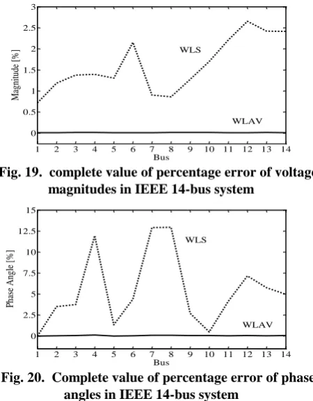
To scrutinize the efficiency of the proposed algorithm under the conventional data, the aggregated errors measurements are initiated by altering the sign of the computed values i.e. the real power flow in 9-14 and the power flow (P & Q) in 9-7. Figs. 19 & 20 show the entire percentage of the approximated errors for magnitude and phase angles with aggregated errors established. Note that the suggested WLAV method produces the smaller error both in the magnitude and phase angles. Besides, the percentage of the aggregated errors of the UPQC control parameters are shown in Table IV. An algorithm performance comparison for these test cases is given in Table V. Note that the state number of A is assessed in this work. Mean squared error of the condition approximation is also resolved. It can also be noticed that the suggested method dispense smaller MSE in the both case studies.

1 2 3 4 5 6 7 8 9 10 11 12 13 14

0 0.5 1 1.5 2 2.5 3

Bus

M

ag

ni

tu

de

[%

]

WLAV WLS

Fig. 19. complete value of percentage error of voltage magnitudes in IEEE 14-bus system

1 2 3 4 5 6 7 8 9 10 11 12 13 14

0 2.5 5 7.5 10 12.5 15

Bus

Ph

as

e

A

ng

le

[%

]

WLAV WLS

[image:5.595.43.292.433.699.2]

Fig. 20. Complete value of percentage error of phase angles in IEEE 14-bus system

Table IV: Percentage Error of UPQC control parameters in IEEE 14-Bus System (Case 2) States

of UPQC

WLS WLAV

Series Source V -3.1384 -0.2536 0.0289 0.0000  5.4139 2.5864 -0.0290 0.1446 Q 7.0150 11.6870 0.0000 0.0000 P 7.4516 7.4516 0.0000 0.0000

Table V: Comparison results

ethod Case Condition

number* MSE Iter.

CPU Time (sec.)

WLS 1 8.5×10

8

4.16×10-2 14 2.68 2 2.6×1010 _3.68×10-1 ₁₅ _2.89

WLAV 1 2.3×10

9

[image:5.595.302.548.549.831.2]

(6)

VI. CONCLUSION

In this paper series compensator and unified power quality conditioner circuits are simulated. In this analysis, we observe the series compensators are simulated for different values of capacitance and inductance. Based on the simulation studies and THD level, it can be recommended that this method is suitable for all the power quality issues Unified power quality controller is simulated for different phase angles of midpoint source. . The solution for the altered IEEE 14-bus system elucidate the suggested algorithm that can be appealed competent for approximating the condition parameters of the power system with UPQC.

REFERENCES

1.M. Noroozian, L. Angquist, M. Ghandhari, G. Andersson, “Power system

improving by FACTS devices,” IEEE Trans. on Power Delivery, vol. 12, no. 4, pp. 1634-1640, Oct. 2010.

2.N.G. Hingorani and L. Gyugyi, Technology and concept of FACTS, IEEE

Press, 2012.

3.L. Gyugyi, C.D. Schauder, S.L. Williams, T.R. Rietman, D.R. Torgerson,

and A. Edris, “UPFC : a novel proposal to power transmission control,” IEEE Trans. on Power Delivery, vol. 10, no. 2, pp. 1085-1097, April 2010.

4.D. Qifeng, Z. Boming, and T.S. Chung, “Estimation of power systems

embedded with FACTS and MTDC systems,” Electric Power Systems Research, vol. 55, no. 3, pp. 147-156, Sept. 2012.

5.X. Bei, and A. Abur, “UPFCs: interior point method,” IEEE Trans. on

Power Syst., vol. 19, no. 3, pp. 1635–1641, Aug. 2010.

6.K.A. Clements, P.W. Davis, and K.D. Frey, “Treatment of inequality

constraints,” IEEE Trans. on Power Syst., vol. 10, no. 2, pp. 567-574, May 2010.

7.A. Monticelli, State Estimation in Electric Power Systems,

Massachusetts, Kluwer Academic Publishers, 2012.

8.M.R. Irving, R.C. Owen, and M.J.H. Sterling, “Power system state

estimation,” Proc. IEE, vol. 125, pp. 879–885, 2010.

9. A. Abur, “Linear programming state estimation,” IEEE Trans. on

Power Syst., vol. 5, no. 3, pp. 894–901, 2000.

10. M.K. Celik, and A. Abur, “A robust WLAV state estimator,” IEEE

Trans. on Power Syst., vol. 7, no. 1, pp. 106–113, Feb. 2006.

11. H. Singh, and F.L. Alvarado, “Weighted least absolute value state

estimation using interior point method,” IEEE Trans. on Power Syst., vol. 9, no. 3, pp. 1478–1484, Aug. 1994.

12. H. Wei, H. Sasaki, J. Kubokawa, and R. Yokoyama, “An interior point

method for power system,” IEEE Trans. on Power Syst., vol. 13, no. 2, pp. 617–623, May 1998.

AUTHORS FROFILE

Dr. S. Sankar, Professor, Department of Electrical and Electronics Engineering, Sriram Engineering College, chennai. Specialized in Power Quality, Electrical Machines, Protection and Switchgears, FACTS, Power system instrumentation.

Dr. M. N. Saravana Kumar, Associate Professor, Department of Electrical

and Electronics Engineering, Erode Sengunthar Engineering College, Erode. Specialized in Power Electronics, Electromagnetic Field computation and Modelling, Power system, High voltage Engineering.

Dr. P. Prabhu, Associate Professor, Department of Mechanical

Engineering, Sriram Engineering College, Chennai. Specialized in Manufacturing Engineering, design if transmission systems.