This is a repository copy of Stochastic network equilibrium under stochastic demand. White Rose Research Online URL for this paper:
http://eprints.whiterose.ac.uk/84671/ Version: Accepted Version
Book Section:
Watling, D orcid.org/0000-0002-6193-9121 (2002) Stochastic network equilibrium under stochastic demand. In: Patriksson, M and Labbe, M, (eds.) Transportation Planning: State of the Art. Applied Optimization, 64 . Kluwer , Dordrecht, Netherlands , pp. 33-51. ISBN 978-1-4020-0546-6
https://doi.org/10.1007/0-306-48220-7_3
© 2002, Kluwer Academic Publishers. This is an author produced version of a paper published in Transportation Planning (Applied Optimization, 64). The final publication is available at Springer via http://dx.doi.org/10.1007/0-306-48220-7_3. Uploaded in
accordance with the publisher's self-archiving policy.
[email protected] https://eprints.whiterose.ac.uk/
Reuse
Unless indicated otherwise, fulltext items are protected by copyright with all rights reserved. The copyright exception in section 29 of the Copyright, Designs and Patents Act 1988 allows the making of a single copy solely for the purpose of non-commercial research or private study within the limits of fair dealing. The publisher or other rights-holder may allow further reproduction and re-use of this version - refer to the White Rose Research Online record for this item. Where records identify the publisher as the copyright holder, users can verify any specific terms of use on the publisher’s website.
Takedown
If you consider content in White Rose Research Online to be in breach of UK law, please notify us by
STOCHASTIC NETWORK EQUILIBRIUM UNDER STOCHASTIC DEMAND
David Watling
Institute for Transport Studies University of Leeds, Leeds LS2 9JT, U.K. Tel: +44 113 233 6612 Fax: +44 113 233 5334
Email: [email protected]
Abstract - A generalisation of the conventional stochastic user equilibrium (SUE) model is developed in order to represent day-to-day variability in traffic flows due to stochastic variation in a) the inter-zonal trip demand matrix, and b) the route choice proportions conditional on the demands. The equilibrated variables in this new problem are the link flow means and covariance matrix. A heuristic solution algorithm is proposed, based on the solution of a sequence of SUE sub-problems. Numerical results are reported from the application of this technique to the Sioux Falls network, and to a second larger network, under the assumption of probit-based choice probabilities. In the Sioux Falls network, a significant impact on mean link flows is observed, and is attributed to a “second order” effect, caused by a large number of small re-routings away from the links whose expected cost is most sensitive to link flow variability. Further investigation reveals that this effect is primarily due to b) above, namely variability in the route choice proportions.
1. INTRODUCTION
The established family of network equilibrium modelsfor representing driver route choice over congested traffic networksconsists of a variety of techniques, the most well-known being the deterministic user equilibrium (DUE) and stochastic user equilibrium (SUE) models, which have
been formulated for both the ‘steady state’ (Sheffi, 1985) and ‘within-day dynamic’ (Ran & Boyce, 1993) cases. A characteristic feature of all models in this family is their use of a deterministic representation for both:
i) the key variables of predictive interest, namely link flows and travel times; and
ii) the primary input variables, namely the inter-zonal travel demand matrix and network characteristics (e.g. free-run speeds/times, capacitites).
The essential difference between the ‘steady state’ and ‘dynamic’ models is that in the latter these input/output quantities are disaggregated into shorter time periods within the day. The more important distinction for the present paper is that between DUE and SUE (whether steady state or dynamic). In the SUE model, drivers are assumed to have perceptual differences in their evaluation of a given travel cost, these differences being most conveniently represented by a pre-specified perceptual probability distribution, distributed across the population of drivers. DUE, on the other hand, assumes a single, mean perception of travel cost. That is to say, in terms of the input/output quantities mentioned above, SUE is no more stochastic than DUE (a point also made by Hazelton, 1998)a preferable choice of term for SUE might have been “disaggregate user equilibrium”, in the spirit of disaggregate demand models (Ortúzar & Willumsen, 1994).
Montgomery & May, 1987; Hanson & Huff, 1988; To, 1990; Willumsen & Hounsell, 1994; Mohammadi, 1997), but the deterministic assumption has prevailed on the basis of their being no clear, tractable way of including it, and based on the belief that variability need not be considered in order to approximate mean conditions. The validity of these beliefs will be addressed in the present paper; in any case, from a policy point of view, this approach leads to difficulties if one wishes to test measures that either may affect such variability and/or are designed to respond to such variability. The study of driver information systems has provided a primary example of such a policy; the major complications that have arisen in matching model predictions with empirical
evidence of response could be said to be a difficulty in separating ‘subjective variation’ (individuals’ preferences and constraints) from the ‘uncertainty’ (the degree to which an individual
fails to satisfy their own preferences/constraints due to predictive errors).
With these comments in mind, the objectives of the present paper are:
1. To formulate a modified version of SUE that is able to represent stochastic variation in travel demand, and the effect of such variation on route choice.
2. To propose a solution algorithm for this modified model.
3. To use this new approach to test the hypothesis that mean traffic conditions are (almost) invariant to the level of demand variability.
In particular, it is noted that the objective is not to build an entirely new modelling paradigm, but to seek a minimal extension to SUE in order to include such variations. In fact, the approach will include stochastic variations in travel demand and its effect on route choice, as well as additional stochastic variation in route choice that occurs even if demand were fixed. In fact, the approach is easily extended to include the effect of stochastic variations in network attributes such as capacities, provided their distribution is independent of traffic conditions; the reason for focusing on stochastic demand (rather than supply) variations is that it is this aspect that is the most complex to represent within a consistent equilibrium framework.
The paper begins by introducing some basic notation and definitions (section 2), and then goes on to make a critique of the existing SUE model (section 3). In section 4, a new formulation of
“equilibrium” is presented for the case of deterministic demand, and in section 5 is subsequently
extended to the case of stochastic demand. In section 6, a heuristic solution algorithm is presented, and in section 7 simulation results are reported for a number of realistic networks.
2. NOTATION
We suppose the network consists of A links indexed a=1,2,...,A, and W inter-zonal (origin-destination) movements indexed k=1,2,…,W. The N possible routes that pass through a link at most once, across all such inter-zonal movements, is indexed by the set {1,2,...,N}, in such a way that the subset of Nk routes
relating to inter-zonal movement k are indexed by the set
Rk r Nj r Nk
j k
: 1 2
1 1
, ,..., .
Define to be an NWpath-movement incidence matrix with elements
rk r k
1
0
if the route indexed relates to interzonal movement
otherwise (r=1,2,...,N; k=1,2,...,W). Then diag(q is an ) NNdiagonal matrix, with diagonal entries from the vector q , such that each row relates to a route, and the diagonal entry for that row is the demand appropriate to that route.
The column vector f of dimension N denotes an assignment of flow to each of the possible routes, with the convex set of demand-feasible non-negative route flow rates denoted by
1 1 2
f N r k
r R
f q k W
k
: for , ,...,
where N denotes N-dimensional non-negative real space. The corresponding convex set of demand feasible link flow rates is
2
vA : v wheref f 1
where is an A N link-path incidence matrix with elements
ar a r
1
0
if link is part of route
otherwise (a=1,2,...,A; r=1,2,...,N).
The cost of travelling along link a at a given link flow rate vector v is denoted by ta(v). These functions
may also themselves be arranged in a column vector, t(v). These link performance functions imply corresponding route cost-flow performance functions
c f( )t(f) (2.1)
where here and throughout the paper, Adenotes the transpose of the matrix A.
Suppose further that for each movement k,
pr( )u : r Rk
is a route choice model describing the probability of a randomly-selected driver on inter-zonal movement k choosing each of the alternative routes when the perceived route costs (averaged across the driver population) are u, and that p(u) denotes these functions across all movements, arranged in a column vector of dimension N. For example, for each movement k it may be assumed that
pr( )u : r Rk
is a random utility modelpr( )u Pr(ur er us es , s Rk , sr) (r Rk; k1 2, ,...,W) where
er : r Rk; k1 2, ,...,W
follow some given joint probability distribution.
We may then state the following well-known definition (Sheffi, 1985).
Definition The route flow rate vector f 1 is a stochastic user equilibrium (SUE) if and only if f diag(q p c f). ( ( )) (2.2) Alternatively, the link flow rate vector v2 is termed a SUE if and only if
v .diag(q p). (t v( )). (2.3)
Corresponding to the usual flow rate variablesq f, and , as defined abovev it will also prove useful to define respective absolute flow variables ~, ~q f and ~v, with elements in the discrete (integer)
duration hours. For example, q1q~ . Throughout the paper, the capitalised versions of
v f v f c, , ~, ~, and tnamely V F V F C, , ~, ~, and T will be used to denote vector random variables of the relevant flow and cost quantities. In terms of the absolute flows, the discrete demand-feasible route flows are given by
~ ~
: ~ ~ , ,...,
1 1 2
f ZN fr qk k W
r Rk
for
where ZN denotes the N-dimensional space of non-negative integers. Similarly, the demand-feasible link flows are given by:
~
2
~v ~v ~f
ZA : where ~f ~1
.3. CRITIQUE OF SUE AND MOTIVATION
As noted in section 1, observations of traffic volumes and travel times indicate considerable day-to-day variability, and so it is not difficult to make a case that these quantities are most appropriately represented as stochastic variables. From a purely deductive philosophy, the fact that SUE neglects significant sources of variability (as DUE does) is perhaps sufficient criticism to warrant the investigation of more sophisticated modelling tools. This is true even if our only interest is in mean network performancedue to the non-linear nature of the interactions between traffic flow, travel times and travel choicerefuting any naïve claim that SUE/DUE necessarily represent mean performance to which variations may subsequently be added. It is worth repeating that the aim of the current work is to characterise mean performance, but within a variable setting.
Taking a more pragmatic viewpoint, however, it is known from the long experience with DUE/SUE models that they have a good degree of explanatory powerthat is to say, they “explain” a good deal of the performance of traffic networks. It is therefore relevant to ask in what way can they be built upon for the purpose of this paper, and in what circumstances can they said to characterise approximate mean performance. Answering this question is a deceptively difficult problem. An appealing pragmatic approach is to assume the SUE link flows represent the mean of independent (between links) Poisson variables, and one could then compute mean costs/times corresponding to these variable flows. One problem with this approach is that is does not represent the high covariances between links that are likely to occur. Two obvious sources of covariance are:
i) in the case of a fixed demand matrix, for two links that are part of alternative routes for a particular inter-zonal movement, the contributions to these link flows from that movement will be negatively correlated (since the route flows are negatively correlated), and for links that are part of the same route there will be a positive correlation;
ii) in the case of stochastic demand, the correlations above must be balanced against positive correlations between the components of link flow for all links used by a particular inter-zonal movement (when demand is high, all route flows are likely to be high).
random utility model evaluated at SUE costs. It is then argued that as all inter-zonal demands become large, the distribution of the flow proportions will become increasingly narrow, and focused on the SUE flows; in the limit, then, as the flow probability distribution becomes focused on a single point, SUE can be viewed as an equilibrium condition on the flow probability distribution. There are a number of difficulties with this line of reasoning:
1. If drivers build up their predictions of travel times/costs from a finite number of past experiencesthese experiences are themselves subject to random variationthen while the distribution of route flows conditional upon the past may be multinomial, the unconditional equilibrium distribution will in general be an over-dispersed multinomial, since the choice probabilities are then stochastic (Hazelton & Watling, 1998).
2. Even if it is possible to assume that drivers’ experiences are sufficiently long that they are able to predict long-run expected costs, so that the choice probabilities are deterministic, then for non-linear link cost-flow performance relationships, SUEin effectively substituting costs at expected flows for expected costscontains an inherent systematic bias (Cascetta, 1989). For convex cost-flow relationships, expected costs are systematically underestimated.
3. As the absolute number of travellers on all inter-zonal movements approaches infinity, then we expect SUE increasingly to approximate SUE mean flow rates, in spite of the misgivings above (Davis & Nihan, 1993). In typical urban, peak period, traffic assignment applications, the zoning system is likely to be sufficiently fine that many inter-zonal movements will have quite a “small” demand, and so the usefulness of the asymptotic result is not clear. In addition, it is important not to confuse the absolute demand with the typical demand input to a traffic assignment model, which is the mean flow rate per hour. The absolute demand depends on both the demand rate and the length of the time period over which this rate is assumed to be valid. A large demand rate on its own is not sufficient, particularly when one considers the current trend in traffic assignment models, towards dynamic models that assign a number of multiple, short time periods.
In response to some of the issues raised here, a radically new approach to traffic assignment modelling was proposed by Cascetta (1989), and extended further by Davis & Nihan (1993) and Cantarella & Cascetta (1995). This approach models the dynamic, day-to-day evolution of travel choices as a discrete time stochastic process, explicitly representing variability in flows and travel
times/costs and their effect on (future) travel choices. “Equilibrium” in this setting refers to a fixed
point condition on the joint probability distribution of network flows. The flexibility of this approach makes it extremely appealing, yet it leaves a practical dilemma. Should we discard the many years of research on understanding and applying traditional network equilibrium approaches (offering an albeit limited but well-controlled modelling environment), in favour of a new approach (the outputs of which are significantly more complex)? Can no use be made of the understanding of traditional equilibrium solution methods? This is a difficult decision, particularly since we would probably be most comfortable selecting conventional equilibrium for some policy tests, and the new approach for others, though this leaves a problem of an inconsistent evaluation framework.
variables the moments of order n and below. A GSUE(1) model therefore equilibrates means only,
and turns out to be an SUE model (regardless of the demand levels, i.e. this is not only a “large sample” result), whilst a GSUE(2) model equilibrates the flow mean and covariance matrix.
This approach, which will form the basis of the remainder of the paper, will shortly be introduced in detail. However, it is useful first to describe the philosophy adopted in the context of random utility theory. In the SUE model (presuming its aim is to estimate mean traffic flows), the cost of each alternative (route) is essentially set to:
Perceived cost = Cost at mean traffic flows + Perceptual difference . (3.1) The cost at mean traffic flows is a deterministic quantity given by the cost-flow performance relationships, and the perceptual differences are randomly distributed (and, in realistic models such as probit, correlated between alternatives). It turns out that the structure of the choices made in the GSUE(2) model could be described as being equivalent to assuming:
Perceived cost = Cost at mean traffic flows + Uncertainty + Perceptual difference (3.2) where the uncertainty is in general a random quantity (between days and between drivers) and is due to the actual variance in traffic conditions. At this level, the objective of the paper can be seen
to be a technique for “fitting” alternative error structures for a random utility model, with mean
flows subsequently predicted by SUE based on this modified error structure.
This description of the approach needs, however, to be clarified in two ways:
1. If the true variance in costs were 2 and drivers’ predictions are assumed to be formed from a large number (m, say) of experiences, then neglecting any correlations between
experiences/alternatives, the variance in the “Uncertainty” is 2
m and so as m this variance
tends to zero. This does not, however, imply that (3.2) approaches (3.1), since unlike “Perceptual difference”, the “Uncertainty” does not have a zero mean; the variability in traffic flows affects
not only the variance in actual costs, but also mean actual costs.
2. From the argument in 1., determining the appropriate correction factor is non-trivial, since in order to determine mean costs at variable flows, the whole flow probability distribution is required. But this leads to a circular argument, since in order to determine the random utility error structure, the (equilibrium) flow distribution is required, but the whole point of specifying the error structure is to determine the equilibrium flows.
The approach will therefore be to deduce conditions that must simultaneously be satisfied by the error structure and the equilibrium flow allocation. This is first considered in the case of a fixed (deterministic) demand, and is then generalised to the case of stochastic demand.
4. EQUILIBRIUM CONDITIONS: FIXED DEMAND
deterministic). For a further elaboration of the proofs and analysis of this section, the reader is referred to Watling (1998).
Let denote the column vector which has elements given by the (unknown) probabilities
Pr(V~ ~) ~ ~v : v2
. thus has dimension equal to the cardinality ~2 of ~2, and is simply a representation of the joint probability distribution of the absolute link flow vector variable V . This ~ distribution is related to the route flow probability distribution (a column vector of probabilities
Pr(F~~f) : ~f ~1
of dimension ~1 ), by , where is a ~2 ~1 matrix with elementsij
1 0
if the route flow referred to by "corresponds" to the link flow
referred to by , in the sense that
otherwise ~ ~ ~ ~ f v v f j
i . (4.1)
Suppose that as in the SUE definition (2.2)/(2.3), a function p(u) is given, which relates the probabilities of a randomly selected driver choosing each of the alternative routes at given route costs u. Then define partitions of this function and the route flow vector F according to the different inter-zonal ~ movements, such that:
~ ~ ~ ~ [ ] [ ] [ ] F F F F 1 2 W
and p u
p u p u p u ( ) ( ) ( ) ( ) [ ] [ ] [ ] 1 2 W
. (4.2)
Now suppose that the route costs uy, where y is a vector of link costs, so that conditionally on y, for each inter-zonal movement k=1,2,…,W independently, each of the ~qk drivers independently chooses between the available routes with probabilities p[ ]k (y). Then the distribution of movement k route flows ~F[k], conditional on random link costs Y, is given by
~
~ (~ , ( )) , ,..., )
[ ] [ ]
Fk Y y Multinomial qk p k y (independently for k1 2 W . (4.3)
The following consistency (equilibrium) condition on the distribution may then be established.
Theorem 1 (Asymptotic equilibrium condition) Suppose that drivers form estimates of actual costs from a random sample
T( )1 ,T( )2 ,...,T( )m
of the link costs from their previous travel experiences, where m is given, T( )j t(1V~( )j ) ( j 1 2, ,..., )m , and
V~( )1 ,V~( )2 ,...,V~( )m
is a sample of independent, identically distributed, demand-feasible link flow vectors. The given cost-flow performance functions ta(1~)v (a=1,2,…,A) are assumed to be bounded for ~v~2. Suppose further that, at given route costs u, the population of drivers chooses independently between the available routes with probabilities p(u). Then asymptotically, as m , the link flow probability distribution satisfies the equilibrium condition:
where ( ) is a vector of dimension ~1 with elements the probabilities Pr( ~F ~f Y E~[ (t V~)]
V
1
where V~ ~ () ~f ~1) (4.5)
where V~ ~ denotes that V has a given probability distribution ~ , where E~[.]
V denotes the
expectation operator with respect to the distribution of V , and where the conditional distribution of ~ ~
F Y is given by (4.3) based on the partition (4.2).
The proof of this theorem, which is given in Watling (1998), essentially hinges on the fact that as the number of experiences m tends to infinity, the variance in the mean of these m i.i.d. experiences will tend to zero, and in the limit implies that the distribution of the mean of the m experiences is focused on the true long run expectation. Hence the corresponding choice probabilities will be deterministic, and the unconditional distribution of F can be approximated by the conditional distribution (4.5), which ~ by hypothesis is formed from a combination of multinomials (4.3).
The derivation of the condition above is very much along the lines of conventional analyses of traffic networks, in the sense that we seek a consistency condition that should reasonably be satisfied, without any specific reference as to how a network may arrive at such a state. For example, in the SUE model (4.2) defined earlier, the hypothesis is that ( , ( ))f c f is in equilibrium if the route proportions given by the behavioural choice model p( ) at costs c f( ) are consistent with flows of f. In addition, by allowing the number of experiences to become very large in Theorem 1, we are effectively assuming a
“well-informed” driver population, again something that is consistent with conventional analyses.
It is worth noting that this does not concur with the notion considered by Cascetta (1989), who viewed equilibrium as something that arises as the result of a dynamical, day-to-day adjustment process: in particular, a discrete time, markov, stochastic process. One example of such a process is where drivers are assumed to learn costs based on an average of their experiences from the last m days, which are then input into a decision model of the form (4.3) in order to determine flows and costs for the current day. That is to say, if V~( )n denotes the random link flow vector on day n, which for given m depends in a time-invariant way on
V~(n1),V~(n2),...,V~(n m )
, and Wm( )n denotes an m-sequence of such variables
~
,~ ,...,~
( ) ( ) ( )
V n m 1 Vn m 2 V n , then we suppose that for n=m+1,m+2,…, the probabilities
Pr(Wm( )n w) : w~2m
are arranged in a column vector ( )n of dimension ~2 m. Then the dynamical process is of the form:( )n (n)
B 1 (n= m+1, m+2,…) (4.6) for some constant (known) transition probability matrix B of dimension ~2 m ~2 . An equilibrium
state of this system is therefore a probability distribution * satisfying
* *
B . (4.7)
Part of ( )n is the marginal probability distributions of each of the constituent vector variablesV~(n j ) (j 1 2, ,..., )m , and in equilibrium these marginal distributions will be identical.
information on the covariances between these variables, and such autocorrelationsi.e. correlations between time periodswill, in general, exist even in equilibrium. The effect is that, as we do not have independence between past experiences, the proof of the asymptotic equilibrium condition (4.4) breaks down (i.e. there is no guarantee that (4.4) will give rise to the correct marginal equilibrium distribution of (4.7)). Indeed, we might reasonably question what we mean by letting m in the markov model, since the whole basis assumes a finite m. On the other hand, initial numerical tests in small artificial networks have indicated that for values of m as low as 5 or 10, (4.4) may approximately characterise the marginals of * in (4.7). At the time of writing, these tests are presently being extended to larger, realistic networks.
Having presented equilibrium conditions, and justified them, a more tractable approximation to them may be deduced (for the proof of the theorem, the reader is again referred to Watling, 1998). For the moment, we are still in the realms of a fixed, deterministic trip demand matrix, but this work will prove to be the basis of the stochastic demand model ultimately developed in section 5.
Theorem 2 (Approximation to Equilibrium Conditions) Consider a network with twice-differentiable link cost-flow functions t(v). Then an approximation to the mean and covariance matrix of an equilibrium probability distribution (4.4) is given by an A-vector and A A matrix satisfying the fixed point conditions:
.
1
diag .
. ( .
( ) ( ( , ))
, ( ( , )))
q p t
q p t
(4.8)
where t( , ) is an A-vector with elements
ta( , ) ta( ) 12 Ha( ), (a 1 2, ,..., )A (4.9) where Ha( ) is the v A A Hessian matrix of ta( ) evaluated at v (for a 1 2, ,...,A), where the scalar product of any two n-square matrices X and Y is denoted by
X Y,
j X Yij ij
n i
n 1 1
and where ( , )q p is a function whose result is an NN block diagonal matrix, with blocks the matrices of dimension Nk Nk:
[ ]k (qk,p[ ]k )qk diag(p[ ]k )p[ ] [ ]kp k (k 1 2, ,...,W) (4.10) where p is partitioned as in (4.2). A pair ( , ) satisfying (4.8) is termed a Generalised Stochastic User Equilibrium of order 2, and is written GSUE(2).
The essential steps in the proof are firstly to deduce a second order Taylor series approximation to the link cost-flow functions, whereby (4.9) may be deduced as an approximation to the expected costs
E~[ ( ~)]
V t V 1
in (4.5). The effect is that on the right hand side of (4.4), only appears through its
mean and covariance matrix, and so these are the only ‘active’ elements of to equilibrate. Hence, on the left hand side, we also deduce the link flow rate mean and covariance matrix, which is related to the absolute link and absolute route flow mean and covariance matrix. This latter mean is diag( ~)q p (note ~q , not q), while the covariance matrix is block diagonal, with blocks [ ]k (~ ,q pk [ ]k )
5. EQUILIBRIUM CONDITIONS: STOCHASTIC DEMAND
Having set up a model in which driver choices and flows may be stochastic, it is a minor extension to allow the inter-zonal demands to be stochastic.
Theorem 3 (Stochastic Demand Equilibrium Conditions) Suppose that the hypotheses of Theorem 2 hold, except that now demand is assumed to be stochastic. Let the given W-vector Q denote the ~ potential demand (number of potential travellers) on each of the inter-zonal movements, and suppose that on any given day, each such potential traveller decides independently to travel with given constant movement-specific probabilities in the W-vector (0k 1, k1 2, ,...,W). Conditional on the choice to travel, a route is subsequently chosen according to probabilities p(.). Then, relative to (4.8), the modified equilibrium conditions on ( , ) are:
.
1
diag .
. ( .
( ) ( ( , ))
, ( ( , )), )
q p t
q p t
(5.1)
where t( , ) and Ha( ) ( av 1 2, ,...,A) are as previously defined, and where ( , , )q p is a function whose result is an NN block diagonal matrix, with blocks:
( , , ) ( )
[ ] [ ] [ ] [ ] [ ]
k qk p k k qk diag p k k pk p k (k1 2, ,...,W) (5.2)
and where the mean demand rate q is related to Q by ~
qk 1 k Q~k. (5.3) A pair ( , ) satisfying (5.1) is termed a Stochastic Demand Generalised Stochastic User Equilibrium of order 2, and is written SDGSUE(2).
Proof The conditions may be derived from Theorem 2, by introducing a dummy “no travel” route for each inter-zonal movement. Under the assumptions of Theorem 3, the Q~k potential travellers on each movement k are multinomially distributed between the non-dummy routes with probabilities
[ ](.) [ ](.)
p k k p k , and so from Theorem 2 with Q 1Q~ we obtain equilibrium conditions of:
.
1
diag .
. . ( ) ( ( , ))
, ( ( , ))
Q p t
Q p t
. (5.4)
(5.1) is then obtained from (5.4) by the substitution (5.3).
One point that is worth noting about (5.1) is what happens as . In that case, with all other variables held fixed, tends to the zero matrix. Then, from (4.9), t( , ) t( ) , and the first condition in (5.1) reduces to an SUE condition on . Now as , for a given mean trip demand rate of qk and travel probability k 0 , then by (5.3) the absolute number of potential travellers
~
6. SOLUTION ALGORITHM
One of the main advantages of the SDGSUE(2) formulation (5.1) is that it allows the direct computation of moments of the equilibrium probability distribution, without having to refer to the underlying distribution. Examining (5.1), it is notable that the first condition has the appearance of an SUE condition (2.3), and this is what motivates the proposed heuristic solution algorithm. In particular, for given , the first condition in (5.1) is indeed an SUE condition on based on modified link cost functions t( , ) . This leads to the obvious strategy of alternately solving an SUE sub-problem in for given , and then updating according to the second SDGSUE(2) condition for the equilibrium route proportions output by the SUE sub-problem. The SUE sub-problem is solved by the method of successive averages (MSA), as described in many standard texts (e.g. Sheffi, 1985).
Formally, the algorithm is as follows:
Initialisation Set ( )0 to the A-vector of zeroes, and ( )0 to the A A zero matrix.
For n=1,2,...:
Auxiliary solution Solve an SUE sub-problem in conditional on (n 1):
. diag( q) . p( t( , (n 1)))
denoting the solution by ( )n and the SUE route proportions by p( )n . Obtain the corresponding estimate of from:
( )n
=-1 . ( q p, ( )n , ) . .
The pair (( )n ,( )n ) is the iteration n auxiliary solution.
Update estimates Update the SDGSUE(2) estimates according to:
( ) ( ) ( ) ( )
( ) ( ) ( ) ( )
n n n n
n n n n
n
n
1 1
1 1
1
1
.
The algorithm is therefore based on twoan ‘inner’ and ‘outer’MSA updating schemes. The inner iterations are used to solve an SUE sub-problem, conditional on the current estimates of the link flow covariance matrix. The outer iterations use the auxiliary solution from the SUE sub-problem to form an updated estimate of a ( , ) satisfying the SDGSUE(2) conditions; at any given outer iteration, this estimate is the average of all auxiliary solutions computed to date. By initialising the covariance matrix to zero, the first outer iteration computes a conventional SUE solution (i.e. based on link cost functions t(v)). This seems a sensible starting point given the asymptotic correspondence, noted in section 5, between SDGSUE(2) mean flows and SUE.
convergence of the MSA algorithm to this solution (Daganzo, 1982; Sheffi, 1985). However, the convergence of the outer iterations is not guaranteed, but if the outer iterations do converge, the resulting estimate will, by construction, be a SDGSUE(2) solution.
This algorithm was implemented in the C language on a personal computer, in which a user-specified number of inner and outer iterations are performed.
7. NUMERICAL TESTS
7.1 Test networks
A probit-based choice probability model p(u) was used in both networks considered, implicitly defined
by assuming that the link cost perceptual “errors” were independent between links, the error for each
link a following a Normal distribution with a mean of zero and a standard deviation t0a, where 0 is a link-independent dispersion parameter and t0a is the free-flow travel cost on link a. A value of
0 3. was assumed throughout. Actual travel time was assumed to be synonymous with actual travel cost. Separable, BPR-type link cost-flow performance functions were used in all cases. All cases were run for a time period duration of 0 25. hours; a choice of, say, 1 hour would generally cause the differences between SUE and SDGSUE(2) flow rates reported below to decrease.
The first network considered was the Sioux Falls one, often used in tests in the literature of network design algorithms, and specified in LeBlanc et al (1975) and Suwansirikul et al (1987). This network is an aggregated representation of the city of Sioux Falls, South Dakota. It consists of some 48 nodes, 124 uni-directional links (including zone centroid connectors), and 24 zones. The demands are fairly evenly distributed across the inter-zonal demand matrix, with trip rates specified in units of thousands of vehicles per day (a total of some 3606 thousand vehicles/day). To convert to peak period, hourly flow ratesa more typical application of assignment modelsa factor of 0.11 was used (as suggested by Suwansirikul et al), both on the demands and on the capacities. Multiplying both by 1000 to obtain units of vehicles/hour yields a total of some 396,660 vehicles/hour in the whole demand matrix. All links in the network have a BPR power of 4.
The second network considered was a rather different one, representing the Weetwood area of Leeds, a commuting corridor consisting of some 70 zones, 440 links and 174 nodes. The inter-zonal demand matrix represents morning peak period trips and is quite sparse; it consists of a total of some 19846 passenger car equivalents per hour. The link-specific BPR powers range from 1.6 to 12.2.
7.2 Test results
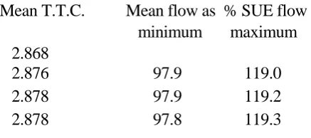
variability implied by travel probabilities of k 0.5, 0.7 and 1 (k 1 2, ,...,W). The comparisons
reported in table 1 are: “Mean T.T.C.”, the mean network-wide total travel cost (=time) in units of 106 vehicle-hours per hour; and “% SUE flow”, the range of SDGSUE(2) mean link flows expressed as a percentage of the corresponding SUE link flows.
Mean T.T.C. Mean flow as % SUE flow minimum maximum
SUE 2.868
[image:14.595.273.492.149.246.2]SDGSUE(2) ( 0 5 . ) 2.876 97.9 119.0 SDGSUE(2) ( 0 7 . ) 2.878 97.9 119.2 SDGSUE(2) ( 1 ) 2.878 97.8 119.3
Table 1: Simulation comparison for Sioux Falls network
There is clearly no appreciable difference between the SDGSUE(2) results in table 1 for different levels of demand variability; that is to say, in the cases considered, while k affects link flow variances it does not appreciably affect mean flows. On a network-wide level, the difference between SUE and SDGSUE(2) total travel costs of around 0.3% is small, but in the intuitive direction expected (SUE, by neglecting variability, will tend to underestimate congestion). The fact that the difference is small is perhaps not surprising, given that the absolute inter-zonal demand levels are quite large (even with
0 25. ) and that SDGSUE(2) mean flows asymptotically approach SUE.
However, this apparent network-wide similarity between SDGSUE(2) and SUE hides a number of significant differences at the level of mean link flows. These small number of links where the difference is greater than 5% are all notably the result of a higher SDGSUE(2) mean flow than SUE flow. Moreover, these links possess the least curvature in the cost-flow relationships, the curvature being the
second derivative function
2 2
t v
a a
, which from (4.9) can be seen to control the effect of variability
on expected cost. Under the node numbering of LeBlanc et al (1975), these links are the two-way links joining nodes 7 to 18, 3 to 12, and 16 to 18 (with the parameter B in table 1 of LeBlanc’s paper effectively measuring the relative curvatures between links at the same flow levels). This effect is balanced by a much larger number of links with small differences, in which the SDGSUE(2) mean flow is slightly smaller (2% at most) than the SUE flow, these occurring on links with the greatest curvature. This latter impact is what one might expect from the SDGSUE(2) model, since at fixed flows, relative to SUE, it will generally inflate costs the most on precisely such links. However the tests have indicated the greatest impact to be a ‘second order’ one, namely the impact made by trips re-routing (in order to avoid such links with inflated costs) on the links that absorb the re-routed flows, with the links with the least curvature attracting a large number of small re-routings. This example illustrates that the SDGSUE(2) model has a potential re-distributional effect on traffic relative to SUE it is not just a correction that uniformly affects all parts of the networkand that this effect may be significant even when the inter-zonal demands are large.
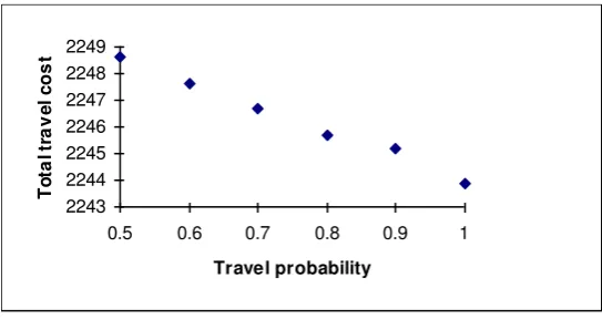
That is to say, since the mean trip rate is fixed in the simulation tests, a decrease in the travel probability represents an increase in variability, and this is seen to increase mean total travel cost. It is worth noting that these small differences are reproducible within different random number seeds (see Table 2), even though their level is outside the level of sampling variability between different seeds. This is achieved by careful use of the random number generator to reduce the variance in results between tests with the same seed (see Rathi, 1992). The more major difference here, like in the Sioux Falls network, is between SUE and the SDGSUE(2) mean results, with a difference in mean total travel cost in the order of 2%. On the individual link level, the range of differences in SDGSUE(2) mean flows relative to the corresponding SUE flows is -8.7% to 53.1% for the case 1 (other cases are similar). However, this is misleading as, unlike the Sioux Falls network, a number of the links carry a much smaller absolute flow of only a few vehicles per hour. In absolute flow terms, the range of differences runs from -27 to 54 vehicles/hour.
2243 2244 2245 2246 2247 2248 2249
0.5 0.6 0.7 0.8 0.9 1
Travel probability
T
o
ta
l t
ra
v
e
l
c
o
s
[image:15.595.161.433.264.408.2]t
Figure 1: Results of SDGSUE(2) model applied to Weetwood network (seed1)
Travel probability () 0.7 0.8 0.9 1.0 SUE Seed1 2246.7 2245.7 2245.2 2243.9 2203.4 Seed2 2244.1 2242.8 2241.6 2240.3 2204.4
Table 2: Effect of travel probability and random number seed on total travel cost (Weetwood)
8. CONCLUSION
It has been demonstrated that stochastic, day-to-day variation in route choice and trip demand can be formulated within the context of an extended network equilibrium framework. The resulting model, which equilibrates link flow means and covariance matrix, is in this way a natural extension of conventional modelling techniques. The heuristic solution algorithm proposed has been shown to be computationally feasible for large realistic networks.
these new models, such as conditions to guarantee existence and uniqueness of equilibrium and the convergence of solution algorithms. Fourthly, the practical use of higher order moments, such as variances and covariances, may be studied in the context of scheme evaluation; the present paper has focused on mean outputs, but how would knowledge of variances affect decision-making? Fifthly, applications of these techniques should be developed, which seem to have particular relevance to policies that respond to variability, such as driver information systems.
ACKNOWLEDGEMENTS
This research was carried out under the support of an Advanced Fellowship from the UK Engineering and Physical Sciences Research Council.
REFERENCES
Cantarella G.E. & Cascetta E. Dynamic Processes and Equilibrium in Transportation Networks: Towards a Unifying Theory. Transpn Sci 29(4), 305-329.
Cascetta E. (1989). A stochastic process approach to the analysis of temporal dynamics in transportation networks. Transpn Res B 23B(1), 1-17.
Davis G.A. & Nihan N.L. (1993). Large population approximations of a general stochastic traffic assignment model. Operations Research 41 (1), 169-178.
Hanson S. & Huff J. (1988). Repetition and day-to-day variability in individual travel patterns. In: Behavioural Modelling in Geography & Planning, ed. by R.C.Golledge & H.Timmermans, Croom Helm, Kent, U.K.
Hazelton M. (1998). Some remarks on stochastic user equilibrium. Transpn Res 32B(2), 101-108. Hazelton M. & Watling D.P. (1998). Approximation methods for over-dispersion and learning processes in markov models of route choice. In preparation.
LeBlanc L.J., Morlok E.K. & Pierskalla W.P. (1975). An efficient approach to solving the road network equilibrium traffic assignment problem. Transpn Res 9, 309-318.
Mohammadi R. (1997). Journey time variability in the London area. Traffic Engineering & Control 38(5), 250-257.
Montgomery F.O. & May A.D. (1987). Factors affecting travel times on urban radial routes. Traffic Engineering & Control, September 1987, 452-458.
Ortúzar J. & Willumsen L.G. (1994). Modelling Transport. Second edition. John Wiley & Sons, Chichester, U.K.
Ran B. & Boyce D.E. (1993). Dynamic Urban Transportation Network Models. Springer-Verlag, Berlin.
Rathi A.K. (1992). The use of common random numbers to reduce the variance in network simulation of traffic. Transpn Res 26B, 357-363.
Sheffi Y. (1985). Urban transportation networks. Prentice-Hall, New Jersey.
To D.K.B. (1990). What happens when it rains. M.Sc. thesis, Institute for Transport Studies, University of Leeds, U.K.
Watling D.P. (1998). A Second Order Stochastic Network Equilibrium Model. Under revision for Transpn Sci.