Turbulent diffusion in rapidly rotating flows with and without stable stratification

This is a repository copy of

Turbulent diffusion in rapidly rotating flows with and without

stable stratification

.

White Rose Research Online URL for this paper:

http://eprints.whiterose.ac.uk/1611/

Article:

Cambon, C., Godeferd, F.S., Nicolleau, F.C.G.A. et al. (1 more author) (2004) Turbulent

diffusion in rapidly rotating flows with and without stable stratification. Journal of Fluid

Mechanics, 499. pp. 231-255. ISSN 0022-1120

https://doi.org/10.1017/S0022112003007055

[email protected] https://eprints.whiterose.ac.uk/ Reuse

Unless indicated otherwise, fulltext items are protected by copyright with all rights reserved. The copyright exception in section 29 of the Copyright, Designs and Patents Act 1988 allows the making of a single copy solely for the purpose of non-commercial research or private study within the limits of fair dealing. The publisher or other rights-holder may allow further reproduction and re-use of this version - refer to the White Rose Research Online record for this item. Where records identify the publisher as the copyright holder, users can verify any specific terms of use on the publisher’s website.

Takedown

If you consider content in White Rose Research Online to be in breach of UK law, please notify us by

DOI: 10.1017/S0022112003007055 Printed in the United Kingdom

Turbulent diffusion in rapidly rotating flows with

and without stable stratification

By C. C A M B O N1, F. S. G O D E F E R D1,

F. C. G. A. N I C O L L E A U2 A N D J. C. V A S S I L I C O S3

1_{Laboratoire de M´ecanique des Fluides et d’Acoustique UMR 5509, ´Ecole Centrale de Lyon,}

69134 Ecully Cedex, France

2_{Department of Mechanical Engineering, University of Sheffield, Sheffield S1 3JD, UK}

3_{Department of Aeronautics, Imperial College, Prince Consort Road, London SW7 2BY, UK}

(Received29 May 2002 and in revised form 12 September 2003)

In this work, three different approaches are used for evaluating some Lagrangian properties of homogeneous turbulence containing anisotropy due to the application of a stable stratification and a solid-body rotation. The two external frequencies are the magnitude of the system vorticity 2Ω, chosen vertical here, and the Brunt–V¨ais¨al¨a frequency N, which gives the strength of the vertical stratification. Analytical results are derived using linear theory for the Eulerian velocity correlations (single-point, two-time) in the vertical and the horizontal directions, and Lagrangian ones are assumed to be equivalent, in agreement with an additional Corrsin assumption used by Kaneda (2000). They are compared with results from the kinematic simulation model (KS) by Nicolleau & Vassilicos (2000), which also incorporates the wave–vortex dynamics inherited from linear theory, and directly yields Lagrangian correlations as well as Eulerian ones. Finally, results from direct numerical simulations (DNS) are obtained and compared for the rotation-dominant case B= 2Ω/N= 10, the stratification-dominant case B= 1/10, the non-dispersive case B= 1, and pure stratificationB= 0 and pure rotation N= 0. The last situation is shown to be singular with respect to the mixed stratified/rotating ones. We address the question of the validity of Corrsin’s simplified hypothesis, which states the equivalence between Eulerian and Lagrangian correlations. Vertical correlations are found to follow this postulate, but not the horizontal ones. Consequences for the vertical and horizontal one-particle dispersion are examined. In the analytical model, the squared excursion lengths are calculated by time integrating the Lagrangian (equal to the Eulerian) two-time correlations, according to Taylor’s procedure. These quantities are directly computed from fluctuating trajectories by both KS and DNS. In the case of pure rotation, the analytical procedure allows us to relate Brownian t-asymptotic laws of dispersion in both the horizontal and vertical directions to the angular phase-mixing properties of the inertial waves. If stratification is present, the inertia–gravity wave dynamics, which affects the vertical motion, yields a suppressed vertical diffusivity, but not a suppressed horizontal diffusivity, since part of the horizontal velocity field escapes wavy motion.

1. Introduction

in many geophysical, industrial and laboratory flows. Direct numerical simulations (DNS) and laboratory experiments have revealed that rapid rotation and stable stratification have highly anisotropic effects on turbulent diffusion (e.g. Britter et al.

1983; Vincent, Michaud & Meneguzzi 1996; Kimura & Herring 1996, 1999; Kaneda & Ishida 2000): turbulent diffusion can be suppressed in one direction but not in others. Surprisingly, in spite of observations in nature, it is difficult to find results of laboratory experiments on turbulent diffusion for rotating flows both with and without stable stratification. (The only experimental work quoted in the recent review of Lagrangian aspects by Yeung (2002) is Jacquin et al. (1990), but turbulent diffusion is only marginally discussed, and not measured, in this paper about rotating turbulence.)

Recent modelling and theoretical approaches by Kaneda & Ishida (2000), Nicolleau & Vassilicos (2000), Kaneda (2000), and Nicolleau & Vassilicos (2003) have been able to explain and predict the suppression of one-particle_†turbulent diffusion along the direction of stratification (vertical) in stably stratified turbulence with and without rapid rotation. All these approaches have in common the use of solutions of the linearized equations of motion. However, Kaneda & Ishida (2000) and Kaneda (2000) base their predictions on Corrsin’s conjecture whereas the kinematic simulations (KS) of Nicolleau & Vassilicos (2000) do not. Corrsin’s conjecture allows the estimation of two-time Lagrangian velocity correlations from a calculation of two-time Eulerian velocity correlations.

Two-time Lagrangian velocity correlations are central quantities in turbulent diffusion because of Taylor’s relation (equation (2.2) in the following section), which expresses the mean-square displacements of fluid particles as a double integral over time of two-time Lagrangian velocity correlations. Taylor’s relation has important physical consequences for turbulent diffusion. In isotropic turbulence, the mean-square displacement behaves proportionally to t2 for short times, in agreement with

a ballistic regime, and evolves proportionaly to t for larger times, in agreement

with a Brownian regime (Taylor 1921). Taylor’s relation can also imply depletion of turbulence diffusion, caused, for example, by vortex trapping. One might expect Lagrangian velocity correlations to oscillate around zero in a vortex, so that the time integral of the Lagrangian correlations are themselves oscillating and decreasing functions of time, thus leading to severe depletion of turbulent diffusion by direct application of Taylor’s integral formula. In this paper, Lagrangian velocity correlations also oscillate in some or all directions as a result of rotation alone or of combined rotation and stratification. We therefore need to calculate these oscillations in order to predict turbulent diffusion and its potential depletion in particular directions. In high-Reynolds-number turbulent flows it is usually the Eulerian velocity statistics that are (more easily) measured experimentally, not the Lagrangian ones, and it is therefore necessary to try to relate the available Eulerian correlations to the desired Lagrangian ones.

Kaneda & Ishida (2000) and Kaneda (2000) calculate these two-time Eulerian correlations using rapid distortion theory (RDT), which is justifiable in the limits of low Froude and Rossby numbers (except for the quasi-geostrophic part of the horizontal motion, for which the nonlinearity does not scale with Rossby or Froude numbers, see Godeferd & Cambon 1994 and Cambon 2001), and use a simplified form of Corrsin’s conjecture to derive two-time Lagrangian correlations. The validity of RDT and the present KS is theoretically limited to times before the appearance

of nonlinear dynamics. Also, polarized vortex tubes and sheets, which are not included in the RDT and KS modelling approaches presented here, might have additional effects on turbulent diffusion which are beyond our reach. Except for DNS results, we demonstrate in this paper how an unstructured velocity field is capable of anisotropically dispersing particles, by considering linear dynamics only. Thorough investigation of how nonlinear velocity field dynamics and polarized flow structures can affect Lagrangian statistics is left for future work.

DNS calculations by Kimura & Herring (1996, 1999) Kaneda & Ishida (2000) confirm the vertical capping of one-particle turbulent diffusion and Nicolleau & Vassilicos (2000, 2002) explain it in terms of energy conservation without recourse to Corrsin’s conjecture. Is there a real need, therefore, for Corrsin’s conjecture in the context of rapidly rotating and/or stably stratified turbulence? And is Corrsin’s conjecture valid in this context? In this paper we attempt to answer these questions by use of theoretical arguments, RDT, KS and DNS, and with particular emphasis on the case of rapid rotation without stratification which has been neglected in the previous studies and which is the one case where conservation of energy arguments are not conclusive with regard to turbulent diffusion. Corrsin’s conjecture concerns the relation between Eulerian and Lagrangian turbulence statistics which is of central and pivotal importance to turbulent diffusion theory. We study the validity of a simplified version of Corrsin’s conjecture (which we call the ‘simplified Corrsin hypothesis’) and its implications for one-particle turbulent diffusion in terms of Taylor’s relation (2.2) in all directions, both parallel and normal to the direction of the rotation vector.

The paper is organized as follows. In _§2 we introduce Corrsin’s conjecture and the simplified Corrsin hypothesis. In_§3 we introduce the governing equations and the ana-lytical and numerical tools used in this study: RDT, KS and DNS. In_§4 the second-order Eulerian velocity correlations are calculated on the basis of RDT solutions, and we use the simplified Corrsin conjecture introduced by Kaneda & Ishida (2000) to predict Lagrangian velocity correlation functions. Also, in this section, we show how the dispersivity of inertial waves modulates, and in fact can even in some cases prevent, the depletion of turbulent diffusion by the oscillations in the flow. At the end of_§4 we use Taylor’s (1921) relation between one-particle second-order statistics and two-time Lagrangian correlations to calculate turbulent diffusivities. The validity of the simplified Corrsin conjecture is tested against KS and DNS in _§5 and in _§6 we compare our turbulent-diffusion theoretical predictions with KS and DNS results obtained at low Rossby and Froude numbers. Particular attention is given to the case of rapidly rotating turbulence without stratification, which has been neglected in the literature, and for which our results are new and perhaps the most surprising. We conclude in _§7.

2. Turbulent diffusion and Corrsin’s conjecture

The position of a particle advected by a velocity field uis given by

˙ x=v_,

where the overdot denotes the substantial derivative following trajectories labelled by the initial (t= 0) position X,

x=x(X, t),

and v_{(t) is the Lagrangian velocity related to the Eulerian velocity field u(x, t) by}

One-particle dispersion in the vertical and horizontal directions is given by(x3−X3)2 and(x1−X1)2+ (x2−X2)2respectively.

Crucial two-time quantities for turbulent diffusion are the covariances ij(t, t′) =

xi(t, t′)xj(t, t′)of the displacement

x(t, t′) =x(t)₋x(t′) =

t

t′

˙ x(s) ds.

Taylor (1921) obtained the well-known relation

ij(t, t′) =

t

t′

ds

t

t′

ds′vi(s)vj(s′), (2.2)

where vi(s)vj(s′) denotes Lagrangian velocity correlations, which differ a priori

from their Eulerian counterparts. Among these Lagrangian integral quantities, 33 and11+22 are particularly informative as they are the mean square of the lengths of particle excursions in the vertical and in the horizontal directions. Let us just recall here that in isotropic turbulence without rotation or stratification, ii(t,0) is

proportional tot2 for short times, in agreement with a ballistic regime, and evolves proportionally to t for larger times, in agreement with a Brownian regime (Taylor 1921).

Taylor’s relation (2.2) means that one-particle turbulent diffusion can be calculated provided that Lagrangian velocity statistics are known. However, it is the Eulerian velocity statistics that are (more easily) usually measured experimentally in high-Reynolds-number turbulent flows, not the Lagrangian ones, and one is therefore confronted with the task of deriving Lagrangian velocity statistics from Eulerian velocity statistics. This is a highly non-trivial task and a central problem of turbulent diffusion which is usually overcome by introducing conjectures and approximations. Corrsin’s conjecture is one important such conjecture which is closely related to Kraichnan’s direct interaction approximation (see Kraichnan 1970, 1977) and which has recently been used by Kaneda & Ishida (2000) to calculate one-particle turbulent diffusion in strongly stratified turbulence. We now describe this conjecture.

Equation (2.1) can also be written

v_{(t) =}

d3_{y u(y, t)δ(y}

−x(X, t)),

and the Lagrangian two-time velocity correlation needed in (2.2) is therefore given by

vi(t)vj(t′)=

d3_y

ui(x(X, t), t)uj(y, t′)δ(y−x(X, t′)). (2.3)

Corrsin’s conjecture (Corrsin 1963) states that, for_|t₋t′_| large enough, (2.3) can be approximated by

vi(t)vj(t′)=

d3yui(x(X, t), t)uj(y, t′)δ(y−x(X, t′)). (2.4)

leads to

vi(t)vj(t′)=

d3kRˆij(k;t, t′)

e−ik·(x(X,t′)−x(X,t))

(2.5)

where

ˆ

Rij(k;t, t′) = (2π)−3

ui(x+r, t)uj(x, t′)e−ik

·r_d3_r.

Equations (2.4) and (2.5) are two different forms of Corrsin’s conjecture neither of which can be of use in practice for calculations concerned with fully turbulent flows. We therefore do not directly study the validity of these equations but of a further simplification which has been introduced by Kaneda & Ishida (2000) and used by them to calculate one-particle vertical diffusion in strongly stratified turbulence. This simplification replaces (2.5) by

vi(t)vj(t′)=

d3_kRˆ

ij(k;t, t′) =ui(x, t)uj(x, t′), (2.6)

and we refer to it as the ‘simplified Corrsin hypothesis’ even though only (2.5) is due to Corrsin.

There is more than one way to derive (2.6) from (2.5) and one series of assumptions is given in Kaneda & Ishida (2000). Effectively, because Eulerian velocity correlations must be dominated by large ‘eddies’ (i.e. small wavenumbers_|k_|), one might expect the high-wavenumber part of the integral (2.5) to make a negligible contribution to the right-hand side of (2.5). The term e−ik·₍x(X,t′₎₋x(X,t)) _{is equal to 1 at k=0and might} be expected to remain close to 1 at small wavenumbers and decrease with increasing wavenumber. This term might therefore be close to 1 in the range of wavenumbers that makes the dominant contribution to the integral in (2.5); on replacing it with 1 in (2.5) one obtains (2.6) without expecting much error, independently of the exact form of the energy spectrum, as long as a logarithmic slope steeper than₋1 is assumed.

3. Background equations and methods

The Navier–Stokes equations using the Boussinesq approximation in a rotating frame are

(∂t+u· ∇)u+ 2Ωn×u+∇p−ν∇2u= b, (3.1)

(∂t+u· ∇)b−χ∇2b=−N2n·u, (3.2)

∇ ·_{u= 0, (3.3)}

for the fluctuating velocityu, the pressurepdivided by a mean reference density, and the buoyancy force b; ν and χ are the kinematic viscosity and thermal diffusivity respectively. The vector n denotes the vertical unit upward direction aligned with both the gravitational acceleration g=₋gnand the angular velocity of the rotating frameΩ_=Ωn. The buoyancy force is related to the fluctuating temperature fieldτ by b=₋gβτ=bn, through the coefficient of thermal expansivity β. With temperature stratification characterized by the vertical gradient γ, the Brunt–V¨ais¨al¨a frequency N=√βgγ appears as the characteristic frequency of buoyancy–stratification. Hence the linear operators in equations (3.1) and (3.2) display the two frequencies N and 2Ω, and we define B = 2Ω/N as a measure of the relative importance of rotation and stratification. Without loss of generality the fixed frame of reference is chosen such thatni=δi3. Therefore, u3 is the vertical velocity component.

3.1. Direct numerical simulation

Using DNS, the system of equations (3.1), (3.2), (3.3) is solved by a numerical spectral collocation method – with 192 Fourier polynomials in each direction of space – in a now classical way for homogeneous turbulence simulations (see e.g. Vincent & Meneguzzi 1991). Prior to solving, the system of equations is rewritten using the vector identity

(u· ∇_)u=ω_×u+ ∇|u 2

| 2 ,

where ω₌∇_{×u is the vorticity. The background rotation 2Ω can therefore be} directly added to the vertical vorticity. The boundary conditions are periodic in all three directions, and the numerical domain is a cubic box of side L0, so that the dimensionless wave vector components are k∗i =ki2π/L0. Spatial derivatives are treated numerically in Fourier space using the pseudo-spectral method and aliasing is treated in spectral space by a spherical truncation of the Fourier components of the fluctuating velocity field, using a 2/3 de-aliasing rule at every time step. The time scheme is third-order Adams–Bashforth, and the viscous term is integrated exactly using the change of variableu′(k) =u(k) exp(νk2_t).

A total of 1000 fluid particles are located initially with a uniform random distribution in the numerical box, and are followed by solving the Lagrangian trajectory equation d(x(X, t))/dt=u(x(X, t), t) at each timestep with a second-order Runge–Kutta scheme. The necessary interpolation for obtaining the velocityu(x(X, t)) at the location of the particle is performed with great accuracy by a Lagrange interpolation scheme which makes use of six points in each direction of space.

2.5

2.0

1.5

1.0

0.5

0 5 10 15 20 25 30 35

B = _ 1 1/10 0 10

t*

E* kin

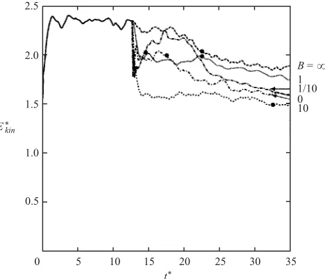
Figure 1. Time evolution of the dimensionless kinetic energy for the entire simulation time

span, for the presented DNS runs.t∗=t /τ is the dimensionless time since the beginning of the isotropic pre-computation, drawn as a solid line (τ= 1.01 is the eddy turnover time at the end of the pre-computation). The anisotropic runs are initiated att∗= 12.59. All the values ofB are plotted, B= 0,1/10,1,10,∞. Black circles indicate the end of computions of Lagrangian statistics, corresponding to different times when non-dimensionalized by the linear timescale (either 2π/N orπ/Ω).

the corresponding (non-dimensional) total kinetic energyE_kin∗ =Ekin/u′2is 1.5 att= 0 (u′₌√_2E

kin/3 being the r.m.s. velocity scale in one direction). The pre-computation of forced isotropic turbulence is performed for a dimensionless time t /τ= 12.59, allowing the turbulent dynamics to set up a realistic distribution with built-up triple correlations (τis the eddy turnover time at the end of the isotropic run). The evolution of the kinetic energy during this stage is shown in figure 1. During this period and after, the Eulerian velocity field is forced by maintaining the large scales – small wavenumbers – at their level at t= 0. This is achieved by multiplying, at every timestep, each spectral coefficient ˆu(k∗) within the spherical spectral shell _|k∗_|<4.52 by E0(k∗_{)/|u(ˆ k}∗_{)|. In so doing, one only modifies the amplitude of the Fourier modes}

B _∞ 10 1 1/10 0

Ro(0) 0.81 0.162 0.81 1.61 _∞

Fr(0) _∞ 1.62 0.81 0.16 0.4

Table 1.Initial Rossby and Froude numbers for DNS runs at different values

of parameterB.

3.2. Linearized dynamical equations

As in RDT, equations (3.1), (3.2) can be linearized for small enough Rossby and Froude numbers. Solutions are easily found in terms of plane waves, and consist of a superposition of steady and oscillating modes of motion, the latter corresponding to dispersive, inertia–gravity, waves (see Cambon 2001). Fourier space is useful for taking into account the divergence-free constraint (3.3), and for allowing exact treatment of the pressure gradient in (3.1). This is important because pressure disturbances are responsible for a coupling of vertical and horizontal velocity components, and for the anisotropic dispersion law of the wavy part of the flow. The solenoidal part of the horizontal field is unaffected by the wave part of the flow and remains constant in the linear inviscid limit: it corresponds to the ‘vortex’ part of the flow in the purely stratified case (see Riley, Metcalfe & Weissman 1981). Accordingly, complete linear solutions (which we call RDT solutions) for the velocity in terms of plane waves may be written as

u(x, t) =exp(ik·x)[A0(k) +A1(k) exp(iσ t) + A−1(k) exp(₋iσ t)] (3.4)

(and similarly forb) where the three vectors Aǫ(k),ǫ= 0,_±1 correspond to the one steady and two wavy modes (see_§4 for details) and are such that Aǫ(k)·_{k = 0 for} incompressibility. The unsigned dispersion frequency σ of inertia–gravity waves is given by

σ =N2_sin2_{θ+ 4Ω}2_cos2_{θ ,}

whereθ(k) is the angle betweenkand the vertical direction. As a consequence of our use of Fourier space and of Aǫ(k)·_{k= 0, the five unknownsu1, u2, u3, p, bin physical} space are now reduced to three in Fourier space, namely two velocity components which we detail in_§4 and the Fourier transform ofb.

Note that two particular cases require special treatment. For pure rotationN = 0 the vector A0 corresponding to the steady part of the flow vanishes in (3.4). And in the case B= 1, it is the dependence of the dispersion frequency on k that vanishes, so that the group velocity is zero for all wavevectors. (This special character of the B = 1 case has also been noted in DNS by Iida & Nagano 1999 and in RDT by Kaneda 2000 and Hanazaki 2002.)

3.3. Kinematic simulation

of the vectors Aǫ(k) and k. (The link of A0, A1 and A−1 to the initial realization is fully specified by equations (4.3)–(4.5), as explained at the end of _§4.1.) At given parameter B, the initial energy spectrum determines the average amplitudes of the vectors Aǫ(k), where these averages are taken over many realizations of the velocity field. Different realizations are obtained by specifying different angular dependences of the vectors Aǫ(k) and k. Great care has to be taken for the angular distribution of modes in these realizations, for the phase and amplitude of oscillation of turbulence to be properly reproduced.

Following Nicolleau & Vassilicos (2000, 2002), additional time decorrelation terms are included in the KS velocity field to yield

u(x, t) =exp(ik·_{x+ iωt)[A}0_{(k) +A}1_{(k) exp(iσ t) +A}−1_{(k) exp(−iσ t)], (3.5)}

where the frequencies ω(k) =λk3_{E(k) withk=|k|and in this paper we investigate} both options, λ _{= 1 and} λ _{= 0. The inclusion of these time decorrelation terms is} intended to model the Eulerian decorrelating effect of the nonlinear advection which we have neglected in the RDT solutions. Indeed, similarly to Nicolleau & Vassilicos (2000) in the purely stratified case, we report in _§5 of this paper that the inclusion of the frequencies ω(k) accelerates the decay of some Eulerian velocity correlation functions obtained by KS of strongly stratified and rotating turbulence, thus leading to more realistic Eulerian correlations. The impact on Lagrangian correlations is shown to be unimportant.

The number of wavevectors over which the summation in every realization of the velocity field (3.5) is carried out is 2000 to 6000, which is much less than in a 1923_DNS. It is therefore practicable to average over many realizations of the flow in KS, whereas the high cost involved in DNS allows the use of only one DNS realization in practice. Accordingly, KS achieves better converged statistics than DNS. It should be stressed that KS is a Lagrangian model of turbulent diffusion and should therefore be used to integrate particle trajectories and generate Lagrangian statistics. Its Eulerian flow structure is flawed as it does not incorporate the persistent characteristic pancake- or cigar-shaped structures that DNS can capture. Of course, the results should coincide with those of analytical RDT when calculating Eulerian velocity correlations, this being an unavoidable validation test.

In our KS, in accordance with Nicolleau & Vassilicos (2000), particles are released at a random time large enough for the velocities to have reached their asymptotic r.m.s. values. This is consistent with KS as a Lagrangian model. Here in contrast to DNS, averages are taken over realizations and in such an approach there is no reason why particles should be released at the same time in each realization.

4. Analytical calculations using RDT

4.1. Projection of the fluctuating fields onto the basis of eigenmodes

The notation and equations in this subsection are the same as in Cambon (2001), which have much in common with Kaneda (2000) (see also Godeferd & Cambon 1994 for details of the mathematical formulation in the stratified case).

In order to unify the mathematical formulation, we shall use a vector ˆw _{whose first}

ˆ

w3 contains the buoyancy force scaled as a velocity:

ˆ

w3= iN−1b.ˆ

In the local frame, the linearized system of equations (3.1)–(3.3) becomes

∂t

_wˆ 1 ˆ w2 i ˆw3

+

0 −_σ

r 0

σr 0 −σs

0 σs 0

ˆ w1

ˆ w2 i ˆw3

=0 (4.1)

or∂twˆ +Mwˆ = 0, where

σr = 2Ωcosθ, σs =Nsinθ, σ =

σ2

r +σs2 (4.2)

are respectively the unsigned dispersion-law frequencies for inertial waves, gravity waves, and inertia–gravity waves.

The system of equations (4.1) is easily solved by diagonalizing the matrix_M. Three eigenmodes are obtainedin the local frame as follows:

N0=





σs/σ

0 σr/σ



, N1= √

2 2



 −σr/σ

i σs/σ



, N−1= √

2 2



 −σr/σ

−i σs/σ





They are related to the eigenvalues 0, σ and ₋σ, respectively. N0 is the stationary mode, which coincides with the quasi-geostrophic mode (QG). Its two components are the horizontal divergence-free part of the velocity, or vortex mode, and one associated with the temperature field. N±1 are the wave modes, also called ageostrophic modes hereinafter in agreement with classic geophysical literature. The wave–vortex terminology was used by Riley et al. (1981) for analysing DNS of stably stratified turbulence, whereas geostrophic and ageostrophic were terms used by Bartello (1995) and Babin, Mahalov & Nicolaenko (1998).

The orthonormal basis of eigenmodes is used to express ˆw _as

ˆ

w₌

ǫ=0,±1 ξǫNǫ

,

with

ξǫ= ˆw·N−ǫ

, ǫ= 0,_±1.

Accordingly, the linearized problem (4.1) obtained from (3.1)–(3.3) is writen (∂t +

iǫσ)ξǫ= 0, whose general solution, given initial values ˆw(k,0), becomes

ˆ

w₍k, t) =

ǫ=0,±1

Nǫ_e−iǫσ t_[N−ǫ_·wˆ(k

,0)]. (4.3)

At this point, one may compute theAǫdefined in (3.4), since they are directly related to the initial conditions through the two kinematic componentsAǫ

i =N ǫ i(N−

ǫ_·wˆ(

k,0)), i= 1,2.

4.2. RDT solutions for second-order Eulerian statistics

From equation (4.3), the linear solution for any statistical Eulerian quantity is readily derived. Second-order statistics are defined through the spectrum of two-point correlationsVij:

1

The RDT equations for Vij are unchanged if one accepts the ‘stretching’ of notation

Vij = wˆ∗i(k, t) ˆwj(k, t′) (instead of the exact equation (4.4)) for linking Vij to its

initial value through the general solution (4.3).

Its components V11(k, t, t′ =t),V22(k, t, t′ =t),V33(k, t, t′= t), V23(k, t, t′= t) are therefore spectral densities of the vortex energy, kinetic wave energy, potential energy, and vertical buoyancy flux, in the absence of system rotation. Only the components with indices 1 and 2 contribute to the spectral tensor ˆRij(k, t, t′) which appears in

(2.5).

Without any calculation, it is obvious that the RDT history of any two-point or single-point correlation can be obtained in a quasi-analytical way provided initial data have simple two-point statistics. For instance, initial three-dimensional isotropic conditions can be chosen as

V11 =V22= Ec(k)

8πk2, V33= Ep(k)

8πk2 , (4.5)

at t = t′ = 0, all other cospectra being zero. Furthermore, the spherically averaged energy spectra can be chosen proportional, such thatEp(k) =αEc(k), for even greater

simplicity. Initial data in KS and DNS are restricted to α = 0 in this article, as in Nicolleau & Vassilicos (2000), but RDT calculations can be easily carried out for any arbitrary value of α, and the particular case α = 1 deserves further investigations. (Non-zero values for α were also considered in RDT by Hanazaki & Hunt 1996.) Using the above initial data, the spectra of Eulerian correlations N−2b(t′_)b(t),

u3(t′)u3(t), andui(t′)ui(t) are calculated from linear combinations of the solution

of theVij integrated over k(see the Appendix). One finds

ui(t′)ui(t)+N−2b(t′)b(t)

=Ekin(0)

1

0

(1₋(1₋α)σ 2

r

σ2 +

2₋(1₋α)σ 2

s

σ2

cosσ(t ₋t′)

dµ

u3(t′)u3(t)

=Ekin(0)

1

0

(1₋µ2) σ2

σr2+ασ

2

s

sin(σ t) sin(σ t′) +σ2cos(σ t) cos(σ t′)

dµ (4.6)

u1(t′)u1(t)+u2(t′)u2(t)=Ekin(0)

1

0

[F(B, µ) +G(B, µ)(cosσ t+ cosσ t′)

+C(B, µ) cosσ tcosσ t′+D(B, µ) sinσ tsinσ t′] dµ, (4.7) with

F(B, µ) =σs2

σs2+ασr2

σ4, G(B, µ) = (1₋α)σ2

rσs2

σ4,

C(B, µ) =σr2

σr2+ασs2

σ4+µ2, D(B, µ) =

σr2(1 +µ2) +ασs2µ2 σ2,

(4.8)

and with σr, σs and σ given by (4.2) and µ= cosθ. The initial amount of kinetic

energy in the whole flow is Ekin(0). It is clear from equations (4.6) to (4.8) that the oscillatory behaviour of Eulerian velocity correlations is modulated by integrations over the wave dispersivitiesσr =σr(µ),σs=σs(µ) andσ =σ(µ).

For pure rotation, N= 0, equations (4.6) and (4.7) reduce to

u3(t′)u3(t)=Ekin(0) 1

0

and

u1(t′)u1(t)+u2(t′)u2(t)=Ekin(0) 1

0

[(1 +µ2) cos 2Ωµ(t₋t′)] dµ.

As for (4.6) and (4.7) the integrands in the above equations are simplified forms of V22(1−µ2) and V11+µ2V22 given in the Appendix. Note from the above equations the important conclusion that both vertical and horizontal Eulerian velocity two-time correlations decay to zero as a result of wave dispersivity.

For pure rotation, setting t = t′ in the above equations we retrieve the well-known result (also reflected by the measure of Reynolds stress anisotropy) that the initial isotropy of the velocity field is conserved by RDT in the sense that u23(t)/[(u21(t) +u22(t))/2] = 1.

4.3. Analytical approach to turbulent diffusion

Only the case of pure rotation is treated in detail in this subsection. Analytical results for the general case,N = 0, will be given in the next two sections, where numerical results are discussed.

Making use of the simplified Corrsin hypothesis (2.6), and therefore equating RDT Eulerian and Lagrangian velocity correlations in Taylor’s equation (2.2), yields

33(s,0) = Ekin(0)

2Ω2 1

0

(1₋µ2)1−cos 2Ωµs

µ2 dµ (4.9)

and

11(s,0) +22(s,0) = Ekin(0)

2Ω2 1

0

(1 +µ2)1−cos 2Ωµs

µ2 dµ, (4.10)

where use has been made of

s

0 dt

s

0

dt′(cos 2Ωµtcos 2Ωµt′+ sin 2Ωµtsin 2Ωµt′) = (1₋cos 2Ωµs)/(2Ω2_µ2_).

The integrals (4.9) and (4.10) result in analytical solutions as follows:_†

˜ x2₃(s)

=33(s,0) = Ekin(0)

4Ω2

4Si(2Ωs)Ωs+ 2 cos 2Ωs₋4 +sin 2Ωs Ωs

(4.11)

and

˜

x2₁(s) + ˜x2₂(s)

=11(s,0) +22(s,0) = Ekin(0)

4Ω2

4Si(2Ωs)Ωs+ 2 cos 2Ωs₋sin 2Ωs Ωs

(4.12)

withSi(t) =t

0u−

1_sinudu.

Equations (4.11) and (4.12) show that, at largeΩt, both the vertical and horizontal r.m.s. displacements behave as√Ωt, or more precisely

˜ x2₃(t)

∼

˜

x2₁(t) + ˜x2₂(t)

∼ E_2Ωkin(0)2 πΩ t (4.13)

using the limitSi(_∞) =π/2. In the limit Ω →0, equations (4.9) and (4.10) tend to

˜ x2₃(t)

= 1 2

˜ x2₁(t)

+ ˜x2₂(t)

= 2 3Ekint

2 _(4.14)

† Integrals similar to (4.9) and (4.10) were assumed to diverge by Kaneda (2000), since he only

looked at the non-oscillating part of their integrand. Convergence atµ = 0 is guaranteed if the

1.0

0.5

0

–0.5

–1.0

0 1 2 3 4 5

f

u1

(0)

u1

(

t

)

g

,

f

u2

(0)

u2

(

t

)

g

,

f

u3

(0)

u3

(

t

)

g

(a₎

Xt_/p

1.0

0.5

0

–0.5

–1.0

0 1 2 3 4 5

(b₎

Xt_/p

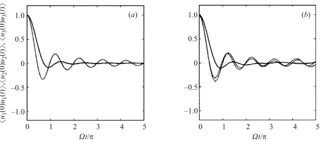
Figure 2. Purely rotating case B = ∞. (a) Analytical RDT for the two-time Eulerian

velocity correlations: , horizontal correlationsu1(0)u1(t)=u2(0)u2(t); , vertical

correlationu3(0)u3(t). (b) KS Eulerian correlations forλ= 0: , horizontal correlations

u1(0)u1(t) and u2(0)u2(t) (as in the following KS plots); , vertical correlation

u3(0)u3(t).

since cos 2Ωµs _∼ 1₋2Ω2_(µs)2_{, for all times. This ballistic behaviour is valid only} at small times, thus pointing to the inadequacy of RDT and/or simplified Corrsin hypothesis in the case without rotation.

Diffusivity in purely rotating turbulence, given by (4.13), is therefore identical to the classical behaviour of isotropic turbulence, after a time large enough to reach the ‘Brownian’ regime for which x˜2 _∝ t. The asymptotic ratio ˜x32/x˜12 shows that isotropy is broken, although not in a dramatic way since it tends towards 2 at large t. The depletion of turbulent diffusion expected from the oscillatory behaviour of the rotating flow is prevented in this case by the wave dispersivity, specifically by integrations over this wave dispersivity as clearly seen in equations (4.9) and (4.10). In other cases of combined rotation with stratification this wave dispersivity simply modulates, and in fact weakens, the depletion of turbulent diffusion due to flow oscillations.

5. The simplified Corrsin hypothesis: Eulerian and Lagrangian two-time correlations from RDT, KS and DNS

In this section we compare Eulerian and Lagrangian two-time correlations obtained by RDT, KS and DNS. Comparisons between Eulerian two-time correlations obtained with RDT, and KS withλ_{= 0, are used to validate our KS and to determine the time} ranges where comparisons are possible.

5.1. Pure rotation, N = 0

1.0

0.5

0

–0.5

–1.0

0 1 2 3 4 5

f

u1

(0)

u1

(

t

)

g

,

f

u2

(0)

u2

(

t

)

g

,

f

u3

(0)

u3

(

t

)

g

(a) 1.0

0.5

0

–0.5

–1.0

0 1 2 3 4 5

(b)

1.0

0.5

0

–0.5

–1.0

0 1 2 3 4 5

f

u1

(0)

u1

(

t

)

g

,

f

u2

(0)

u2

(

t

)

g

,

f

u3

(0)

u3

(

t

)

g

(c)

Xt/p

1.0

0.5

0

–0.5

–1.0

0 1 2 3 4 5

(d)

Xt/p

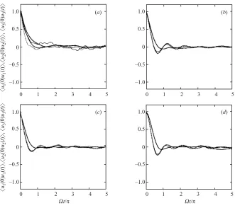
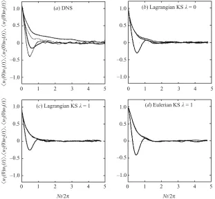
Figure 3.Purely rotating caseB=_∞. , two-time horizontal velocity correlations; ,

vertical correlation, for (a) DNS results with Eulerian correlations drawn with heavy lines, and Lagrangian ones with thin lines; (b) KS Lagrangian correlations (λ_{= 0); (c) KS Lagrangian} correlations (λ_{= 1); (d) KS Eulerian correlations with}λ_{= 1.}

and compare with figures 2b and 3d respectively). Our DNS results (see figure 3a) confirm the validity of the simplified Corrsin hypothesis in the horizontal direction. They are less conclusive in the vertical direction, as we can observe a rather clear difference between the Eulerian and the Lagrangian vertical correlations from about Ωt /π≃ 1. However, one must take into account the lack of statistical sampling for the Lagrangian velocity correlations, which are computed using 1000 fluid particles in the DNS, which is much less than the 1923 _{collocation points used to calculate} the Eulerian correlations. This lack of sampling causes a difference in the oscillation amplitude between horizontal Eulerian and Lagrangian correlations, and may be the cause of (or at least contribute to) the observed departure in the vertical. Moreover, no ensemble average is performed for the DNS results, so that large overall oscillations in the correlations are present, which would tend to be smoothed out when averaging with results from other runs with different initial turbulent phases.

5.2. General case with stable stratification

In the stratified case, with and without rotation, initial isotropy is not conserved by RDT forsingle-timeEulerian correlations, in the absence of initial equipartition, that is when (1/2)N−2_b2_{(0)= Ekin(0)/2 orα = 1. The asymptotic value of 2u}2

with the collapse of vertical motion, and the above ratio could be larger than 1 for different values ofα and/or different values ofB (see Cambon 2001).

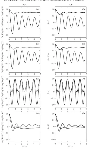
In the general case for whichNis not zero,two-timeEulerian correlations calculated by RDT depend on t and t′ separately (for all α = 1), and not only through their difference, as in the case of pure rotation and in the isotropic case. Correlations in the vertical direction decrease to zero for largeNt, whereas they tend to a non-zero plateau for the horizontal direction according to the non-zero value ofF(B, α, µ) in (4.7) and (4.8). The main difference with the case of pure rotation is that the horizontal two-time velocity correlation (4.7) tends to a non-zero limit asNtincreases, whereas its vertical counterpart decreases to zero. Hence, two-time Eulerian correlations become strongly anisotropic at sufficiently large separation times. The Eulerian two-time correlations obtained from RDT and KS with λ _{= 0 are compared in figure 4 for a choice of} values ofB, and the comparison is satisfactory.

The simplified Corrsin hypothesis is found to hold in KS in the vertical direction for all finite values of B and for both values of λ_{. This is illustrated in figures 5–8} for Eulerian and Lagrangian vertical and horizontal correlations in KS for different B values and λ_{= 0 or}λ_{= 1: figure 5 forB = 0, figure 6 for B= 1/10, figure 7 for} B = 1, figure 8 for B = 10. It is interesting to note that the Lagrangian two-time correlations are unaffected by the value of λ except in the vertical direction for the caseB= 1. In the horizontal direction the simplified Corrsin hypothesis is recovered by KS only for λ= 1: in figures 3, and 5 to 8 Lagrangian and Eulerian correlations look quasi-identical, and even those in the horizontal direction have the same decay to zero forλ= 1. Whenλ= 0, the horizontal Eulerian two-time correlations obtained by KS and by RDT do not decay to zero, as shown in figure 4, which means that the simplified Corrsin hypothesis is not valid in that case. In the non-dispersive B = 1 KS results, the difference between Eulerian correlations for λ_{= 0 and} λ_{= 1} is therefore striking (figures 4f and 7d). This effect of λ _{on the decay of Eulerian} velocity correlations is also present in KS results for isotropic turbulence (Ω=N= 0) as shown in figure 9. Figure 9 shows clearly that Eulerian velocity correlations are equal to 1 for all time in KS when λ _{= 0 but decay with time when} λ _{= 1. From} tracking of fluid particles in the laboratory, Mann & Ott (2002) have found some evidence that the simplified Corrsin hypothesis is valid in isotropic turbulence.

Our DNS results confirm, at least qualitatively, that the simplified Corrsin hypothesis is valid in the vertical direction for all values of B but seem to invalidate this hypothesis in the horizontal directions. In the stratification-dominant cases, from figures 5 and 6 the conclusion is very clear: apart from small differences due to statistical aliasing, Eulerian and Lagrangian DNS correlations are very close in the vertical direction, and also compare very well with KS evolutions. On the other hand, horizontal DNS correlations separate at about half a Brunt–V¨ais¨al¨a period

Nt/2π ≃ 0.5, for both B = 0 and B = 1/10 cases. For the non-dispersive case (figure 7), while Eulerian and Lagrangian DNS correlations are nearly identical at the initial stage, one observes a slight separation of the horizontal correlations. For the rotation-dominant case B= 10, the simplified Corrsin hypothesis seems well-verified in both the vertical and the horizontal directions (figure 8).

6. Results for turbulent diffusion

6.1. Pure rotation

1.0

0.5

0

–0.5

–1.0

0 1 2 3 4 5

f u1 (0) u1 ( t ) g , f u2 (0) u2 ( t ) g , f u3 (0) u3 ( t ) g

(a)

Nt/2p RDT 1.0 0.5 0 –0.5 –1.0

0 1 2 3 4 5

B

= 0

(b)

KS 1.0 0.5 0 –0.5 –1.0

0 1 2 3 4 5

f u1 (0) u1 ( t ) g , f u2 (0) u2 ( t ) g , f u3 (0) u3 ( t ) g

(c) 1.0

0.5

0

–0.5

–1.0

0 1 2 3 4 5

B

= 1/10

(d)

1.0

0.5

0

–0.5

–1.0

0 1 2 3 4 5

f u1 (0) u1 ( t ) g , f u2 (0) u2 ( t ) g , f u3 (0) u3 ( t ) g

(e) 1.0

0.5

0

–0.5

–1.0

0 1 2 3 4 5

B

= 1

(f)

1.0

0.5

0

–0.5

–1.0

0 1 2 3 4 5

f u1 (0) u1 ( t ) g , f u2 (0) u2 ( t ) g , f u3 (0) u3 ( t ) g

(g) _1.0

0.5

0

–0.5

–1.0

0 1 2 3 4 5

B

= 10

(h)

Nt/2p

Figure 4.Eulerian two-time velocity correlations forB= 0: , horizontal; , vertical.

Nt/2p 1.0

0.5

0

–0.5

–1.0

0 1 2 3 4 5

f

u1

(0)

u1

(

t

)

g

,

f

u2

(0)

u2

(

t

)

g

,

f

u3

(0)

u3

(

t

)

g

(a) DNS 1.0

0.5

0

–0.5

–1.0

0 1 2 3 4 5

(b) Lagrangian KS k = 0

Nt/2p 1.0

0.5

0

–0.5

–1.0

0 1 2 3 4 5

f

u1

(0)

u1

(

t

)

g

,

f

u2

(0)

u2

(

t

)

g

,

f

u3

(0)

u3

(

t

)

g

(c) Lagrangian KS k = 1 _1.0

0.5

0

–0.5

–1.0

0 1 2 3 4 5

(d) Eulerian KS k = 1

Figure 5. Two-time horizontal velocity correlations for the purely stratified case B = 0:

, horizontal; , vertical. (a) DNS results for Eulerian correlations are drawn with thick lines, and thin lines for Lagrangian correlations; (b) Lagrangian correlations from KS withλ_{= 0; (c) Lagrangian correlations from KS with}λ_{= 1; (d) Eulerian correlations from} KS withλ_{= 1.}

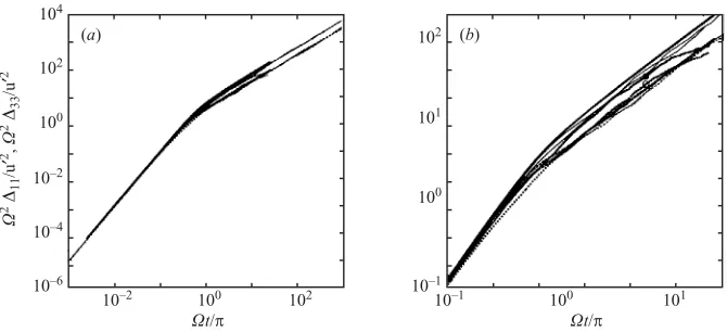
different values of the Rossby number Ro = 0.04 and 0.08, and the DNS case at B =_∞. To be precise,Ω2x˜2₁/u′2 and Ω2x˜2₃/u′2 are plotted against Ωt /π, whereby a very good collapse of the curves is obtained. Moreover, we observe the following two features: the evolution ultimately leads to a Brownian behaviour, and the ratio of vertical to horizontal diffusivity tends towards the analytically predicted value of 2. RDT and KS with λ _{= 1 exhibit this value exactly, whereas in DNS this ratio} only reaches the smaller value 1.4. Our DNS run exhibits the long-time Brownian behaviour as well, although for Ωt /u′2 & 10 dispersion in the DNS seems to drop a little as observed on the zoomed figure 10(b), departing from the behaviour of RDT and KS. This can be due to nonlinear effects, but also to the fact that vertical and horizontal diffusivity depend on the particular realization of initial phases of the turbulent structures in the flow. There again, one is confronted by the classical problem of obtaining converged ensemble averages, which require many realizations, particularly in the case of rotating turbulence.

6.2. General case with stable stratification

Nt/2p 1.0 0.5 0 –0.5 –1.0

0 1 2 3 4 5

f u1 (0) u1 ( t ) g , f u2 (0) u2 ( t ) g , f u3 (0) u3 ( t ) g

(a) DNS 1.0

0.5

0

–0.5

–1.0

0 1 2 3 4 5

(b) Lagrangian KS k = 0

Nt/2p 1.0

0.5

0

–0.5

–1.0

0 1 2 3 4 5

f u1 (0) u1 ( t ) g , f u2 (0) u2 ( t ) g , f u3 (0) u3 ( t ) g

(c) Lagrangian KS k = 1 1.0

0.5

0

–0.5

–1.0

0 1 2 3 4 5

(d) Eulerian KS k = 1

Figure 6.As figure 5 but for the stratification-dominant caseB= 1/10.

Nt/2p 1.0

0.5

0

–0.5

–1.0

0 1 2 3 4 5

f u1 (0) u1 ( t ) g , f u2 (0) u2 ( t ) g , f u3 (0) u3 ( t ) g

(a) DNS 1.0

0.5

0

–0.5

–1.0

0 1 2 3 4 5

(b) Lagrangian KS k = 0

Nt/2p 1.0

0.5

0

–0.5

–1.0

0 1 2 3 4 5

f u1 (0) u1 ( t ) g , f u2 (0) u2 ( t ) g , f u3 (0) u3 ( t ) g

(c) Lagrangian KS k = 1 1.0

0.5

0

–0.5

–1.0

0 1 2 3 4 5

(d) Eulerian KS k = 1

Figure 8. As figure 5 but for the rotation dominant caseB= 10.

t 1.0

0.5

0

–0.5

–1.0

0 1 2 3 4 5

f

u1

(0)

u1

(

t

)

g

,

f

u2

(0)

u2

(

t

)

g

,

f

u3

(0)

u3

(

t

)

g

Lagrangian k _{= 0}

Eulerian k _{= 0}

Eulerian k _{= 1}

Lagrangian

k _{= 1}

Figure 9.Correlations of velocity for isotropic turbulence, computed from KS:

, vertical; , horizontal.

(a)

104

102

100

10–2

10–4

10–6

10–2 ₁₀0 ₁₀2

t/p

2

11

/u

′

2,

2

33

/u

′

2

(b)

102

101

100

10–1

10–1 ₁₀0 ₁₀1

t/p

Figure 10.One-particle non-dimensional diffusion for pure rotation (B = ∞), vertical

Ω233/u′2 ( ) and horizontal Ω211/u′2 ( ). The thin lines (extending to

Ωt /π ≃ 1000) show results obtained with KS, with two different values of the Rossby number, Ro = 0.08 and 0.04; in each set, the horizontal dispersion is the lowest of the two. Heavy lines indicate analytical RDT with the simplified Corrsin hypothesis ( , vertical dispersion; , horizontal dispersion), and DNS results, identified on the close-up plot (b) by a black circle for the vertical dispersion, and an open circle for the horizontal dispersion. On the large-scale plot (a), thet2 and t laws are easily identified, respectively at short and long times.

Looking at its horizontal counterpart, the leading term, which is obtained by replacing (4.7) in (2.2) and invoking the simplified Corrsin hypothesis, shows that the square of the horizontal displacement is proportional to [1

0 F(B, µ) dµ]t 2_{. Such}

a ‘ballistic’ behaviour in the horizontal direction, already found by Kaneda (2000), disagrees with KS results withλ_{= 1, which exhibit an eventual Brownian behaviour} at largest time (Nicolleau & Vassilicos 2003), and preliminary DNS results tend to confirm this KS long-time behaviour, although many more runs would be needed for a complete confirmation.

In figure 11, we collect all the analytical results obtained from RDT with the simplified Corrsin hypothesis. An interesting feature is the presence of a transient t zone, and the larger the B the larger the zone, although the t2 _{law always ‘catches} up’, except for the pure rotation case. Horizontal dispersion in DNS contains hints of this transientt zone, in the sameB range, although the time duration of this zone is much shorter.

6.3. Physical discussion

When the dynamics is not completely dominated by rapid oscillations connected to dispersive waves, the analytical procedure only captures a ‘ballistic’ regime at larger times, since quasi-steady motion prevails. This is the case for the rotating non-stratified flow, in which inviscid RDT yields only pure steady Eulerian correlations. It is also the case for horizontal dispersion forN = 0, since the pure divergence-free horizontal velocity field, which contributes to the quasi-geostrophic mode, disperses the particles with increasing r.m.s. displacement at increasing Nt. This effect only leads to a ‘ballistic’ regime when predicted by our analytical procedure, but to a more realistic ‘Brownian’ regime with KS (especially withλ_{= 1), and DNS seems to} support the latter results.

102

101

100

10–2

10–3

10–4

10–2 ₁₀0 ₁₀1

t ₁₁

10–1 103 104

10–1 ₁₀2 ₁₀3

105

Figure 11. One-particle diffusion11(t) =22(t) calculated with analytical RDT, using the

simplified Corrsin hypothesis, for the different parameter cases: , B = 0; , B = 1/10; , B = 1; · · ·_{, B = 10; , B = ∞. The two segments show t and t}2 power laws.

and λ = 1 are in agreement in this case in predicting a ‘Brownian’ behaviour with a constant ratio of the smaller horizontal diffusivity to the vertical diffusivity. The level of the turbulent diffusion obtained in KS depends on the Rossby and Reynolds numbers, in a way which is briefly mentioned in the next section.

Crude scaling arguments based on the Rossby radius, often used in rotating flows, yield the wrong conclusion that for horizontal dispersion a plateau may be expected (see for instance the sketch in figure 18 in Jacquinet al.1990). When the nonlinearity is important, however, it could have a different impact on the vertical and on horizontal diffusivities in pure rotation, a problem which remains open and which motivates future refined DNS calculations.

Finally, it is important to underline that the theoretical and computational tools used here are completely different from the Lagrangian stochastic models. For instance, the classical approach for diffusion in stratified fluids by Csanady (1964) uses a stochastic model in which the pressure is treated as a random force, in contrast with our KS, RDT, and pseudo-spectral DNS approaches, where the pressure field is naturally accounted for by the divergenceless property of the whole flow.

7. Concluding remarks

Using analytical linearized theory, the stochastic kinematic simulation model (KS), direct numerical simulations, and comparisons thereof, we have drawn conclusions pertaining to the validity of Corrsin’s hypothesis in stably stratified/rotating turbulent flows, and to the diffusion laws, summed up as follows.

We begin with our evaluation of the simplified Corrsin hypothesis by KS.

(ii) In the horizontal direction, Eulerian two-time velocity correlations decay to 0 only as a result of nonlinearity (i.e. when λ_{= 1 which models the decorrelation due} to Navier–Stokes nonlinearity) when B is not infinite. WhenB =_∞, the horizontal Eulerian two-time correlations decay to zero as a result of the dispersivity of inertial waves (and therefore for both λ = 0 and λ = 1). In the presence of stratification (i.e. at finite values ofB) part of horizontal motion is not affected by inertia–gravity waves, so that the horizontal Eulerian two-time correlations do not decay to zero except when the effect of decorrelation by Navier–Stokes nonlinearity is factored into the KS model by λ _{= 1. However, Lagrangian two-time velocity correlations} decay to 0 even when the nonlinearity of the velocity field is severely depleted, that is even when λ_{= 0 in KS, because of the time-decorrelation that is inherent in the} integration of particle trajectories. Hence, the simplified Corrsin hypothesis is not valid in the horizontal when the nonlinearity is depleted in the flow itself. In the rotating case without stratification, the simplified Corrsin hypothesis is always valid in the horizontal as a result of the dispersive inertial waves that affect the whole flow. Our DNS results do not invalidate the simplified Corrsin hypothesis in the vertical in all cases of stratification with or without rotation. These results are not conclusive for the case of pure rotation in the vertical direction. In the horizontal direction, all our DNS runs with dominant stratification show that the simplified Corrsin hypothesis fails after a short time. This might suggest that the impact of Navier– Stokes nonlinearity on the validity of this hypothesis is complex and not easy to model: the simple nonlinear model incorporated in KS through random frequencies, with λ = 1, seems to be sufficient to validate the simplified Corrsin hypothesis for horizontal motion, but DNS results are not in agreement for long enough time. Long-time behaviour being the hardest to compute accurately both in KS and DNS of rotating and/or stratified turbulence (and in fact more so in DNS), we chose to take a careful stance and not draw definitive conclusions from this failure of DNS to fully support the simplified Corrsin hypothesis in the horizontal direction.

It is a direct consequence of Taylor’s (1921) relation that any mechanical effect producing negative loops in two-time Lagrangian correlations can reduce turbulent diffusion. In the context of this paper, these effects are caused by the stratification and/or rotation and are modulated, sometimes even prevented, by wave dispersivity. Accordingly, concerning anisotropic diffusivity, we have observed the following.

(i) In the case of rotation without stratification, RDT and the simplified Corrsin hypothesis along with Taylor’s (1921) relation imply that both the horizontal and vertical diffusion is Brownian for long times and ballistic for short times and that the ratio of the vertical to the horizontal turbulent diffusivities is 2. KS confirms the ballistic and Brownian behaviours, as well as the ratio 2, but predicts a different scaling which depends on both the Rossby and Reynolds numbers. KS results suggest a scaling of x˜2/L2 _∼ Ro2u′t /L (Nicolleau & Vassilicos 2003), in contrast to the Ro u′t /Ldependence which derives from the analytical relationship (4.13).

λ_{= 0 is in keeping with the fact that the simplified Corrsin hypothesis is validated} by KS in the horizontal for λ_{= 1 but not for}λ_{= 0.}

J. C. V. acknowledges support from the Royal Society. Direct numerical simulations were performed on the Fujitsu VPP5000 of CEA, thanks to computing time allocated by the “Centre Grenoblois de Calcul Vectoriel.”

Appendix. Analytical or semi-analytical results for damped oscillations

The Craya–Herring frame of reference is defined by

e1= k×n |k_×n_|, e

2₌ k k ×e

1_{, e}3₌ k

k, (A 1)

except for kn, where it coincides with the fixed frame of reference. Note that the spectral components of the velocity/temperature vector ˆw _{= ˆw1e}1 _{+ ˆw2e}2 _{+ ˆw3e}3

written in this frame have counterparts in physical space which can be directly associated with the oscillating motion and the potential vorticity. Accordingly, w2 represents twice the total, kinetic + potential, energy.

From (4.3), (4.4) and (4.5) one finds

Vii(k, t, t′) =

E(k,0) 8πk2

1₋(1₋α)σ 2

r

σ2 +

2₋(1₋α)σ 2

s

σ2

cosσ(t₋t′)

. (A 2)

From (A 1) ˆu3= ˆw2e23 and ˆw3 = iN−1b, withˆ ni =δi3, e13 = 0 ande23=−sinθk.

From (4.3) ˆw2 = ˆwt2=0cosσ t −(σrwˆt1=0+σswˆt3=0) sinσ t /σ, so that using (4.4) and (4.5)

V22(k, t, t′) = E 8πk2

cosσ tcosσ t′+ σ 2

r +ασ

2

s

σ2 sinσ tsinσ t

′

, (A 3)

from which the integrand of (4.6), or (1₋µ2)V22, is derived. From ˆw3 = ˆwt1=0σrσs/

σ2(cosσ t₋1) + ˆwt=0

3 (σr2+σs2cosσ t)/σ2+ ˆwt2=0(σs/σ) sinσ t one obtains

V33(k, t, t′) = E 8πk2

H(B, x)₋(1₋α)σ 2

rσ

2

s

σ4 (cosσ t+ cosσ t

′₎

+L(B, x) cosσ tcosσ t′+σ 2

s

σ2sinσ tsinσ t

′

. (A 4)

Finally, V11 is obtained by subtracting (A 3) and (A 4) from (A 2), so that

V11(k, t, t′) = E 8πk2

F(B, µ) + (1₋α)σ 2

rσs2

σ4 (cosσ t+ cosσ t

′₎

+C(B, µ) cosσ tcosσ t′+σ 2

r

σ2sinσ tsinσ t

′

, (A 5)

with

H(B, µ) =σr2

σs2+ασr2

σ4, L(B, µ) =σs2

σr2+ασs2

σ4

F(B, µ) =σ2

s

σ2

s +ασr2

σ4_{, C(B, µ) =σ}2

r

σ2

r +ασs2

σ4_,

(A 6)

and (4.7) is derived from its integrandV11+µ2V22.

laws: conservation of total energy in any orthonormal frame of reference w_i∗wi =

ǫ=0,±1ξǫ∗ξǫ, and conservation ofQG energy ξ0∗ξ0. Finallyu2

3andb2are given by integrals over the angular variableµ. Their history shows damped oscillations (due to the integral of emiσ t_{, m =}

±1,_±2) and constant terms (m = 0 due to contributions from ξ0∗ξ0, ξ1∗ξ1, ξ−1∗ξ−1). Hence, at least the asymptotic values can be analytically calculated. Of course, other simplifications due to semi-axisymmetry (axisymmetry without mirror symmetry) have to be used (u2₁ = u2₂, etc.), as well as optimal sums and differences of solution equations. Reynolds stress components and buoyancy variance are

u2₃= 2Ekin(0)

3 [P + (1−α)fv(N t, B)] (A 7)

N−2b2= 2Ekin(0)

3 [Q+ (1−α)fb(N t, B)] (A 8)

u2₁+

u2₂= 2Ekin(0)

3 [3(1 +α/2)−P−Q−(1−α)(fv(N t, B) +fb(N t, B))] (A 9) with

P = 3 4

1

0

1₋µ2

B2_µ2_{+ (1−µ}2₎[2B 2

µ2+ (1₋µ2)(1 +α)] dµ, (A 10)

Q= 3 4

1

0

1₋(1₋α)B

4_µ4_{+ (1−µ}2₎2_/2

(B2_µ2_{+ 1−µ}2₎2

dµ, (A 11)

fv(N t, B) =

3 4

1

0

(1₋µ2)2

B2_µ2_{+ (1−µ}2₎cos[2N t

B2_µ2_{+ (1−µ}2_{)] dµ, (A 12)}

fb(N t, B) =−

3 4

1

0

₍₁

−µ2)2

2(B2_µ2_{+ 1−µ}2₎2 cos[2N t

B2_µ2_{+ (1−µ}2_)]

+ 2B

2_µ2_(1−µ2₎

(B2_µ2_{+ 1−µ}2₎2cos[N t

B2_µ2_{+ (1−µ}2_)]

dµ. (A 13)

P(α, B) andQ(α, B) are easy to calculate, especially forB = 0 (no rotation),B = 1 (no wave dispersivity), pure rotation (singular case). For instance P = (1 +α)/2 for B= 0, and P = (3 + 2α)/5 for B= 1. The function f(N t, B) can be shown to give damped oscillations.

REFERENCES

Babin, A., Mahalov, A. & Nicolaenko, B.1998 On nonlinear baroclinic waves and adjustment of

pancake dynamics.Theor. Comput. Fluid Dyn.11_{, 215–235.}

Bartello, P.1995 Geostrophic adjustment and inverse cascades in rotating stratified turbulence.

J. Atmos. Sci.52, 4410–4428.

Britter, R. E., Hunt, J. C. R., Marsh, G. L. & Snyder, W. H.1983 The effect of stable stratification

on turbulent diffusion and the decay of grid turbulence. J. Fluid Mech.127_{, 27–44.}

Cambon, C.2001 Turbulence and vortex structures in rotating and stratified flows. Eur. J. Mech.B

Fluids20, 489–510.

Corrsin, S. 1963 Estimates of the relations between Eulerian and Lagrangian scales in large

Reynolds number turbulence. J. Atmos. Sci.20_{, 115–119.}

Csanady, G. T.1964 Turbulent diffusion in a stratified fluid. J. Atmos. Sci.21_{, 439–447.}

Godeferd, F. S. & Cambon, C.1994. Detailed investigation of energy transfers in homogeneous

Hanazaki, H.2002 Linear processes in stably and unstably stratified rotating turbulence. J. Fluid Mech.465_{, 157–190.}

Hanazaki, H. & Hunt, J. C. R. 1996 Linear processes in unsteady stably stratified turbulence.

J. Fluid Mech.318_{, 303–337.}

Iida, O. & Nagano, Y.1999 Coherent structure and heat transfer in geostrophic flow under density

stratification. Phys. Fluids11, 368–377.

Jacquin, L., Leuchter, O., Cambon, C. & Mathieu, J. 1990 Homogeneous turbulence in the

presence of rotation. J. Fluid Mech.220_{, 1–52.}

Kaneda, Y.2000 Single-particle diffusion in strongly stratified and/or rapidly rotating turbulence.

J. Phys. Soc. Japan69, 3847–3852.

Kaneda, Y. & Ishida, T. 2000 Suppression of vertical diffusion in strongly stratified turbulence.

J. Fluid Mech.402_{, 311–327.}

Kimura, Y. & Herring, J. R. 1996 Diffusion in stably stratified turbulence. J. Fluid Mech. 328_, 253–269.

Kimura, Y. & Herring, J. R. 1999 Particle dispersion in rotating stratified turbulence. InProc. FEDSM99 3rd ASME/JSME Joint Fluid Engineering Conf.FEDSM99-7753.

Kraichnan, R. H.1970 Diffusion by a random velocity field. Phys. Fluids13_{, 22–31.}

Kraichnan, R. H. 1977 Lagrangian velocity covariance in helical turbulence. J. Fluid Mech. 81, 385–398.

Lundgren, T. S. & Pointin, Y. B.1976 Turbulent self-diffusion. Phys. Fluids19_{, 355–358.} Mann, J. & Ott, S. 2002 An experimental test of Corrsin’s independence hypothesis and related

assumptions. Number XXVII in General Assembly, Nice, France. EGS.

Nicolleau, F. & Vassilicos, J. C. 2000 Turbulent diffusion in stably stratified non-decaying

turbulence. J. Fluid Mech.410, 123–146.

Nicolleau, F. & Vassilicos, J. C. 2003 Kinematic simulation for stably stratified and rotating

turbulence. J. Fluid Mech.(to be submitted).

Orszag, S. A. & Patterson, G. S.1972 Numerical simulation of three-dimensional homogeneous

isotropic turbulence. Phys. Rev. Lett.28, 76–79.

Riley, J. J., Metcalfe, R. W. & Weissman, M. A.1981 Direct numerical simulations of homogeneous

turbulence in density-stratified fluids. InProc. AIP Conf. on Nonlinear Properties of Internal

Waves(ed. B. J. West), pp. 79–112. American Institute of Physics.

Taylor, G. I.1921 Diffusion by continuous movements.Proc. Lond. Math. Soc.(2)20_{, 196–211.} Vincent, A. & Meneguzzi, M.1991 The spatial structure and statistical properties of homogeneous

turbulence. J. Fluid Mech.225, 1–20.

Vincent, A., Michaud, G. & Meneguzzi, M.1996 On the turbulent transport of a passive scalar

by anisotropic turbulence. J. Fluid Mech.8_{, 1312–1320.}