Multilayer Active Shell Mirrors
Thesis by
John Steeves
In Partial Fulfillment of the Requirements for the Degree of
Doctor of Philosophy
California Institute of Technology Pasadena, California
2015
c
2015
Acknowledgements
First and foremost I would like to thank my advisor, Professor Sergio Pellegrino, for providing me with the opportunity to work in this exciting field of research. Your willingness to spend time with students, encouragement to keep pushing forward when challenges arise, and excitement for all things mechanics is unparalleled. My time as a graduate student has been extremely enjoyable and I attribute it to this wonderful environment that you provide. I would also like to thank Professor Guruswami Ravichandran, Professor Dennis Kochmann, and Professor Joel Burdick for their time and willingness to serve on my committee.
I would like to acknowledge the many current and former members of the Space Structures Laboratory who have been wonderful research partners throughout the past 4 years. I especially want to thank Dr. Keith Patterson who provided invaluable mentorship, particularly in the early years, as well as Dr. Marie Laslandes who was patient enough to introduce me to optics. It has been a pleasure working with you both. I would also like to thank my office mate, Dr. Xin Ning, for many in-depth and often late night discussions on mechanics which seemed to increase in frequency during the days leading up to my defense.
I have had the pleasure of collaborating with many people throughout my graduate career. A special acknowledgment is required for Dr. David Redding, Dr. Samuel Case Bradford, James Kent Wallace, Dr. Scott Basinger, and Dr. Troy Barbee for the direct collaboration on this project. I have enjoyed our interactions immensely and look forward to working with you all further. I would also like to thank Dr. Andrew Shapiro, Dr. Harish Manohara, Dr. Risaku Toda, Dr. Greg Davis, John Baker, and Mark Thomson for the continual support of our research efforts.
I thank the staff at GALCIT, specifically Petros Arakelian, Joe Haggerty, Kathleen Jackson, Dimity Nelson and Christine Ramirez. I would especially like to thank Petros Arakelian for the many hours spent troubleshooting in lab.
I would like to acknowledge the Natural Sciences and Engineering Research Council of Canada (NSERC), NASA JPL, and the Keck Institute for Space Studies (KISS) at Caltech for funding our research. I would especially like to thank Michelle Judd from KISS who provides unparalleled student support at Caltech.
Abstract
This thesis presents a novel active mirror technology based on carbon fiber composites and replication manufacturing processes. Multiple additional layers are implemented into the structure in order to provide the reflective layer, actuation capabilities and electrode routing. The mirror is thin (<1.0 mm), lightweight (2.7 kg/m2) and has large actuation capabilities. These features, along with the associated manufacturing processes, represent a significant change in design compared to traditional optics. Structural redundancy in the form of added material or support structures is replaced by thin, unsupported lightweight substrates with large actuation capabilities.
Several studies motivated by the desire to improve as-manufactured figure quality are performed. Firstly, imperfections in thin CFRP laminates and their effect on post-cure shape errors are studied. Numerical models are developed and compared to experimental measurements on flat laminates. Techniques to mitigate figure errors for thicker laminates are also identified. A method of properly integrating the reflective facesheet onto the front surface of the CFRP substrate is also presented. Finally, the effect of bonding multiple initially flat active plates to the backside of a curved CFRP substrate is studied. Figure deformations along with local surface defects are predicted and characterized experimentally. By understanding the mechanics behind these processes, significant improvements to the overall figure quality have been made.
Studies related to the actuation response of the mirror are also performed. The active properties of two materials are characterized and compared. Optimal active layer thicknesses for thin surface-parallel schemes are determined. Finite element simulations are used to make predictions on shape correction capabilities, demonstrating high correctabiliity and stroke over low-order modes. The effect of actuator saturation is studied and shown to significantly degrade shape correction performance.
Contents
Acknowledgements iii
Abstract iv
1 Introduction 1
1.1 Background and Motivation . . . 1
1.1.1 Replicated Mirror Technologies . . . 2
1.1.2 Active Mirror Technologies . . . 3
1.2 Active Mirror Concept . . . 5
1.3 Outline of Thesis . . . 6
2 Active Mirror Design 8 2.1 Requirements on Mirror . . . 8
2.1.1 Figure Accuracy . . . 8
2.1.2 Surface Roughness . . . 9
2.2 Mirror Substrate . . . 10
2.3 Reflective Front Surface . . . 11
2.4 Active Layer . . . 12
2.5 Electrode Routing Layer . . . 14
2.6 Mounting . . . 14
2.7 Overview of Fabrication Process . . . 15
3 Imperfections in Symmetric Thin-Ply Composites 17 3.1 Introduction. . . 17
3.1.1 Background . . . 18
3.1.2 Objective and Scope . . . 18
3.2 Spatially-Uniform Imperfections. . . 19
3.2.1 Problem Formulation . . . 19
3.2.1.1 Identification of Relevant Parameters . . . 21
3.2.2.1 Thickness Variations. . . 22
3.2.2.2 Ply Misalignments . . . 23
3.2.2.3 Thermal Gradients During Cure . . . 24
3.2.3 Numerical Modeling . . . 25
3.2.3.1 Uniform Variations in Ply Thickness . . . 27
3.2.3.2 Variations in Ply Alignment . . . 27
3.2.3.3 Thermal Gradients. . . 29
3.2.3.4 Sensitivity Analysis . . . 29
3.2.4 Shape Error Measurements . . . 30
3.3 Spatially-Varying Imperfections . . . 32
3.3.1 Shape Error Measurements (Mid Spatial Frequency) . . . 33
3.3.2 Sources of Imperfections . . . 33
3.3.3 Imperfection Characterization. . . 34
3.3.3.1 Ply Thickness . . . 34
3.3.3.2 Fiber Misalignments . . . 35
3.3.4 Numerical Modeling . . . 36
3.3.4.1 Results . . . 37
3.3.4.2 Comparison to Experiments . . . 39
3.3.5 Model Extensions. . . 40
3.4 Discussion of Results . . . 42
4 Multi-Ply CFRP Laminates 44 4.1 Laminate Choice . . . 44
4.1.1 Measured Shape Errors . . . 46
4.2 Reduction of Shape Errors. . . 46
4.2.1 Low-Temperature Cure Cycle . . . 47
4.2.2 Deformable Mandrel Surface . . . 49
4.2.2.1 Problem Definition. . . 49
4.2.2.2 Measurements of Nominal Shape Errors . . . 50
4.2.2.3 Description of Deformable Mandrel Apparatus . . . 51
4.2.2.4 Verification of Mandrel Deformation . . . 52
4.2.2.5 Shape Correction . . . 53
4.3 Discussion of Results . . . 54
5 Nanolaminate Bonding 57 5.1 Overview of Nanolaminates . . . 57
5.3 Nanolaminate Bonding . . . 61
5.3.1 Thermal Co-Cure. . . 61
5.3.2 Room-Temperature Cure . . . 62
6 Figure Errors from Active Layer 65 6.1 Background and Motivation . . . 65
6.2 Model Overview . . . 66
6.2.1 Deformation Boundary Conditions . . . 67
6.3 Step 1: Stress distribution due to Spherical Deformations . . . 69
6.3.1 Circular Plates . . . 69
6.3.2 Octagonal Plates . . . 72
6.4 Step 2: Deformation due to Bonding . . . 75
6.4.1 Global Deformation . . . 77
6.4.2 Experimental Measurements . . . 82
6.4.3 Local Deformation . . . 82
6.5 Deformation Upon Uniform Actuation . . . 86
6.6 Measurement of Cross-Pattern . . . 91
6.7 Tessellated Active Layer . . . 92
6.8 Transverse Shear Effects . . . 95
6.8.1 In-Plane Deformation . . . 96
6.8.2 Out-of-Plane Deformation . . . 97
6.9 Discussion of Results . . . 99
7 Actuation Response 101 7.1 Active Materials . . . 101
7.1.1 Piezoelectric Ceramics . . . 101
7.1.2 Electrostrictive Ceramics . . . 106
7.2 Surface Parallel Actuation Scheme . . . 108
7.2.1 Sizing of Active Layer . . . 108
7.3 Patterned Electrodes . . . 110
7.3.1 Optimal Electrode Pattern . . . 111
7.4 Shape Error Correction . . . 112
7.4.1 Numerical Model . . . 113
7.4.2 Predicted Performance. . . 114
[image:7.612.70.545.64.688.2]8 Mirror Experiments 121
8.1 Wavefront Characterization . . . 121
8.2 Description of Metrology Setup . . . 123
8.3 Verification of Projected Hartmann Setup . . . 125
8.4 Shape Correction Experiments . . . 128
8.4.1 Active Mirror Prototype . . . 128
8.4.2 Measured Influence Functions . . . 130
8.4.3 Figure Correction. . . 130
8.4.4 Stage 2 Attempt . . . 131
9 Conclusions 133 9.1 Summary of Results . . . 133
9.2 Unique Contributions . . . 135
9.3 Improvement of Figure Accuracy . . . 136
9.4 Follow-On Work . . . 137
A Spatial Filtering of Surface Shapes 138
B ABD Matrices of Considered Laminate Orientations 141
C Active Layer Bonding Convergence Study 143
List of Figures
1.1 a) Advanced Technology Large Aperture Space Telescope (ATLAST) concept. b) Autonomous
Assembly of a Reconfigurable Space Telescope (AAReST) concept. . . 1
1.2 a) 1.0 m dia. parabolic composite mirror from Composite Mirror Applications [6]. b) 150 mm. dia. CFRP mirror with a reflective nanolaminate facesheet [7]. . . 3
1.3 Front and back surfaces of the Actuated Hybrid Mirror (AHM) [14]. . . 4
1.4 Backside of thin 100 mm dia. mirrors from a) Cilas [16]. and b) Patterson, K. [17].. . . 4
1.5 Exploded view of active mirror concept. . . 5
2.1 Ratio of specular reflectance, Rs, to total reflectance, Rt, at normal incidence. . . 9
2.2 Schematic of fiber print-through. . . 11
2.3 Schematic of resin-rich cure process used to mitigate fiber print-through. . . 12
2.4 Schematic of nanolaminate bonding process used to mitigate fiber print-through. . . 12
2.5 Backside of a 150 mm dia. active mirror prototype containing four PZT-5A plates with a custom electrode pattern. . . 13
2.6 Backside of an active CFRP mirror after electrode routing layer integration. . . 14
2.7 Bare CFRP substrate mounted using spherical magnets.. . . 15
2.8 Overview of fabrication process. . . 15
3.1 Folding concept envisioned for extremely thin lightweight mirrors. . . 17
3.2 Through-thickness coordinate definition for Classical Lamination Theory. . . 19
3.3 Micrograph of laminate cross-section displaying ply thickness measurements. . . 23
3.4 Schematic of ply grinding process used to image internal plies. . . 23
3.5 Image of line detection algorithm used to perform fiber measurements.. . . 24
3.6 Fiber angle measurements of external and internal plies used to assess ply alignment accuracy. 25 3.7 (a) Schematic of thermocouple placement on specimen. (b) Thermocouple readings during autoclave cure. . . 26
3.9 Results of NL FEA (solid) and CLT prediction (dashed) for uniform variations in ply orientation.
a) Laminate curvatures and b) resulting shape error magnitudes. . . 28
3.10 Results of NL FEA (solid) and CLT prediction (dashed) for thermal gradients during cure. a) Laminate curvatures and b) resulting shape error magnitudes. . . 29
3.11 RMS error as a function of imperfection magnitude. Results are normalized by a) the full-scale (FS) values and b) the measured (meas) values in Table 3.3. . . 30
3.12 Measured shape errors of the three constructed laminates. . . 31
3.13 Calculated shape errors due to measured imperfection magnitudes. . . 32
3.14 Post-cure shape error of a 4-ply [0◦/90◦]slaminate. . . 32
3.15 Measured mid-spatial frequency errors of the constructed laminates. . . 33
3.16 Sources of spatially varying imperfections due to tow-spreading: a) thickness variations and b) fiber misalignments. . . 34
3.17 Thickness measurements performed using cross-sectional micrographs. . . 34
3.18 a) In-plane image of terminal ply displaying significant variations in fiber direction. b) Measured fiber orientation distribution for the T800 material. . . 35
3.19 Schematic of numerical model used to model spatially-varying imperfections. . . 36
3.20 Schematic of method used to model ply thickness variation. . . 36
3.21 Schematic of method used to model fiber misalignment . . . 37
3.22 Shape error due to spatial variations in ply thickness. . . 38
3.23 Shape error due to spatial variations in fiber orientation. . . 38
3.24 Predicted mid-spatial frequency shape errors due to measured imperfection magnitudes. . . 39
3.25 Shape error dependence on nominal ply thickness. . . 40
3.26 Shape error dependence on curing temperature.. . . 41
3.27 Shape error dependence on nominal laminate orientation. . . 42
4.1 Normailized in-plane (A11) and bending (D11) stiffness at various orientations. . . 45
4.2 Measured shape errors for a) 8-ply, b) 16-ply, and c) 32-ply laminates . . . 46
4.3 Autoclave cure cycle displaying nominal (black) and low-temperature (red) profiles. . . 47
4.4 Measured shape errors for 16-ply substrates using a) the nominal and b) the low-temperature cure cycle. . . 48
4.5 Schematic of deformable mandrel concept.. . . 50
4.6 Shape measurements of CFRP substrates cured atop mandrel with zero imposed actuation. . . 51
4.7 CAD schematic of deformable mandrel. . . 52
4.8 Fabricated deformable mandrel. . . 53
4.9 Zernike coefficients of deformable mandrel shape at various levels of actuation. . . 54
5.1 250 mm diameter nanolaminate deposited on a polished 2.0 m ROC spherical mandrel. . . 58
5.2 Gaussian curvature of a) Cylinder, b) Hyperboloid (Saddle/Astigmatism) and c) Spherical cap. 59 5.3 a) Measured shape and b) Gaussian curvature of a free-standing nanolaminate. . . 60
5.4 Top-view of CFRP + nanolaminate facesheet after a thermal co-cure displaying significant thermal distortions. . . 61
5.5 Successful integration of nanolaminate onto a 200 mm dia. CFRP substrate. . . 63
5.6 White light scanning interferometer (Veeco Wyko) measurements of a) a bare CFRP sub-strate after replication displaying significant fiber print-throughand b) a mirror prototype after nanolaminate integration showing complete mitigation of fiber print-through (Ra: 2.2 nm). . . 63
6.1 Overview of model displaying two substrates having dissimilar geometry, undergoing deforma-tion to a common interface (Step 1) and determinadeforma-tion of the new, post-bonded equilibrium configuration (Step 2).. . . 66
6.2 Reference surface and thickness definition of the CFRP and PZT parts. . . 67
6.3 Permitted boundary conditions for non-linear finite element model.. . . 68
6.4 Radial element displaying mid-plane and bending stress components.. . . 70
6.5 Normalized mid-plane stress distribution in a) radial and b) circumferential directions due to spherical deformations of an initially flat circular plate (Note difference in colorscale). . . 71
6.6 a) Radial and b) circumferential stress ratios (mid-plane / bending stress) along the radial coordinate due to spherical deformations of an initially flat circular plate. . . 72
6.7 Coordinate system for octagonal plate.. . . 73
6.8 Normalized mid-plane stress distribution in a) radial and b) circumferential directions due to spherical deformations of an initially flat continuous octagonal plate (Note difference in colorscale). 73 6.9 Normalized mid-plane stress distribution in a) radial and b) circumferential directions due to spherical deformations of initially flat sections of an octagonal plate (Note difference in colorscale). 74 6.10 a) Radial and b) circumferential stress ratios (mid-plane / bending stress) along the radial coordinate atθ= 45◦for the continuous plate (solid) and discontinuous patches (dashed). . . 75
6.11 Abaqus model displaying continuous CFRP substrate and four discrete PZT patches modeled using conventional shell elements (S4R). . . 77
6.12 8-ply substrates: Global deformation of CFRP substrate after bonding a) a continuous plate or b) four discrete patches of PZT. . . 78
6.13 16-ply substrates: Global deformation of CFRP substrate after bonding a) a continuous plate or b) four discrete patches of PZT. . . 78
6.14 32-ply substrates: Global deformation of CFRP substrate after bonding a) a continuous plate or b) four discrete patches of PZT. . . 79
6.16 Deformation of a 16-ply CFRP substrate with an initial radius of curvature, R, of 2.0, 4.0 and
10.0 m (a), b), c) respectively) after bonding a continuous sheet of PZT to its backside. . . 81
6.17 Deformation of a 16-ply CFRP substrate with an initial radius of curvature, R, of 2.0, 4.0 and
10.0 m (a), b), c) respectively) after bonding a four discrete patches of PZT to its backside. . . 81
6.18 Normalized change in curvature due to the bonding process in the radial direction atθ= 45◦ for the continuous plate (solid) and discontinuous patches (dashed). . . 81
6.19 Measurement of out-of-plane deformation of an 8-ply CFRP substrate after bonding 4 PZT
plates to the backside. . . 82
6.20 Mesh refinement for central portion of CFRP substrate. . . 83
6.21 8-ply substrates: Local out-of-plane deformation after bonding process for a) 0.25 mm, b) 1.0
mm, c) 2.0 mm gap widths. . . 84
6.22 16-ply substrates: Local out-of-plane deformation after bonding process for a) 0.25 mm, b) 1.0
mm, c) 2.0 mm gap widths. . . 84
6.23 32-ply substrates: Local out-of-plane deformation after bonding process for a) 0.25 mm, b) 1.0
mm, c) 2.0 mm gap widths. . . 84
6.24 Profile of gap deformation over central portion of CFRP substrate for a) 8-ply, b) 16-ply and
c) 32-ply substrates... . . 85
6.25 Comparison of X (solid) and Y (dashed) gap deformation profiles for 8-ply CFRP substrates. . 86
6.26 8-ply substrates: Comparison of global deformation upon actuation at 200µfor a) continuous PZT and b) discrete PZT patches. . . 86
6.27 16-ply substrates: Comparison of global deformation upon actuation at 200µfor a) continuous PZT and b) discrete PZT patches. . . 87
6.28 32-ply substrates: Comparison of global deformation upon actuation at 200µfor a) continuous PZT and b) discrete PZT patches. . . 87
6.29 8-ply substrates: Local out-of-plane deformation upon actuation at 200 µ strain for a) 0.25 mm, b) 1.0 mm, c) 2.0 mm gap widths. . . 88
6.30 16-ply substrates: Local out-of-plane deformation upon actuation at 200 µstrain for a) 0.25 mm, b) 1.0 mm, c) 2.0 mm gap widths. . . 88
6.31 32-ply substrates: Local out-of-plane deformation upon actuation at 200 µstrain for a) 0.25 mm, b) 1.0 mm, c) 2.0 mm gap widths. . . 89
6.32 Profile of local out-of-plane deformation upon actuation at 200µstrain for a) 8-ply, b) 16-ply, and c) 32-ply substrates . . . 90
6.33 Comparison of X (solid) and Y (dashed) gap deformation profiles after actuation for 8-ply
6.34 White light scanning interferometer (Zygo Zemapper) measurement of the center portion of a
mirror substrate displaying evidence of the cross-pattern produced from the four discrete PZT
plates. . . 92
6.35 Overview of model showing a 1.0 m hexagonal mirror with 150 mm PZT patches arranged in a continuous tesselation.. . . 92
6.36 Figure deformation due to uniform actuation (200 µstrain). a) Base curvature change, and b) shape after removal of the first 36 Zernike modes. . . 94
6.37 Local deformations at gap locations due to uniform actuation (200µstrain). . . 94
6.38 Overview of continuum shell model used to capture transverse shear deformations. . . 96
6.39 In-plane deformation in a) x-direction and b) y-direction due to actuation. . . 97
6.40 Continuum shell element model displaying out-of-plane deformation due to uniform in-plane actuation of the PZT at 200µstrain. . . 98
6.41 Constant x and y deformation profiles due to 0.25 mm gap over central portion of CFRP substrate. Comparison between continuum and conventional shell models.. . . 98
7.1 Non-centrosymmetric attice structure of PZT displaying dipole direction. . . 102
7.2 a) Random domain orientation before poling. b) Orientation of domains through poling electric field. c) Remnant polarization after removal of poling field. . . 102
7.3 Directional convention for domain polarization and electric field. . . 103
7.4 Measured in-plane strain of PZT-5A displaying domain switching due to high electric fields.. . 104
7.5 Measured in-plane strain of PZT-5A over operating electric field range (± 0.8 MV/m). a) Response of material directly after poling showing accumulation of strain and b) centered data after multiple cycles showing a repeatable but hysteretic response. . . 105
7.6 Centrosymmetric lattice structure of PMN-PT. . . 106
7.7 Schematic of electrostrictive domain orientation. a) Random domain orientation in base state. b) Spontaneous orientation due to applied electric field. c) Return to base state and random domain orientation upon removal of electric field.. . . 107
7.8 Measured in-plane strain of PMN-PT over operating electric field range. . . 107
7.9 Schematic of surface-parallel actuation scheme. . . 108
7.10 Active layer thickness ratio, t∗, on maximum actuation curvature change. . . 110
7.11 Actuation of discrete regions using patterned electrodes.. . . 111
7.12 Optimized electrode pattern displaying unique electrode positions. . . 112
7.13 Schematic of shape correction process. . . 112
7.14 Comparison of central influence function for a) 8-ply, b) 16-ply, and c) 32-ply designs. . . 114
7.16 Shape correction results for a 16-ply mirror showing: a) 5µm RMS of initial astigmatic error, b) the residual error of 55 nm RMS after correction (considering 95% of the overall aperture),
and c) the corresponding actuator voltages required for correction showing a large degree of
saturation. . . 115
7.17 Comparison of astigmatism correction for 8, 16, and 32-ply mirror designs. . . 115
7.18 Correctability of Zernike modes for 8, 16 and 32-ply mirror designs. . . 116
7.19 Zernike stroke for 8, 16 and 32-ply mirror designs. . . 117
7.20 Schematic of interdigitated electrodes producing in-plane actuation strains in the direction of applied electric field. . . 118
7.21 Schematic of orthotropic actuation concept. . . 118
7.22 Radial and circumferential influence functions from the orthotropic actuation scheme (Results shown for 16-ply design). . . 119
7.23 Comparison of correctability for isotropic and orthotropic actuation schemes (Results shown for 16-ply design). . . 120
8.1 Schematic depiction of a Shack-Hartmann wavefront sensor displaying spot displacements from a distorted wavefront. . . 121
8.2 Schematic of Projected Hartmann test showing nominal beamlet reflection from a perfectly spherical mirror (blue) and one with local slope errors (red). . . 122
8.3 Picture of custom metrology apparatus used for mirror experiments. . . 124
8.4 Ray-trace diagram of custom metrology apparatus demonstrating the two optical paths. . . 125
8.5 Spot pattern produced using the Projected Hartmann apparatus showing deviations from a regular grid. . . 125
8.6 Comparison of Projected Hartmann measurement and speckle photogrammetry measurement displaying good agreement over high-amplitude astigmatic modes. . . 126
8.7 Comparison of Projected Hartmann measurement and Shack-Hartmann measurement (HASO3-76) displaying good agreement over low-amplitude mid-spatial frequency modes. . . 127
8.8 Front surface of fully-integrated Carbon Shell Mirror (CSM) prototype. . . 128
8.9 Schematic of control system used for closed-loop figure control. . . 129
8.10 Measured influence functions using the Projected Hartmann setup. . . 130
8.11 Figure error before and after closed-loop correction displaying 0.52µm of residual error. . . 131
A.1 a) Unfiltered surface measurement displaying dominating low-spatial frequency curvature terms.
b) Power spectral density (PSD) of surface shape after implementation of FFT. c) High-pass
Gaussian spatial filter. d) Filtered surface measurement after implementation of high-pass filter
and iFFT revealing mid-spatial frequency features. . . 140
List of Tables
2.1 Requirements on mirror figure at various wavelengths . . . 9
2.2 Material properties of unidirectional T800 and M55J carbon fibers embedded in ThinPregT M 120EPHTg-1 epoxy (Vf ≈50%). . . 10
2.3 Material properties for PZT-5A. . . 13
3.1 Orthotropic properties of unidirectional T800 carbon fibers embedded in ThinPregT M 120EPHTg-1 epoxy (Vf ≈60%). . . 22
3.2 Ply thickness measurements. . . 23
3.3 Full-scale and standard deviations of imperfections. . . 30
3.4 Imperfection magnitudes used for simulation comparison . . . 31
3.5 Imperfection magnitudes used for experimental comparison . . . 39
3.6 Comparison of measured and calculated shape errors. . . 40
4.1 Considered CFRP laminate orientations . . . 44
4.2 Reduction in laminate bending stiffness . . . 45
4.3 Measured RMS shape error for 16-ply laminates. . . 48
5.1 Mean Gaussian curvature and radius of curvature of the free-standing nanolaminate and depo-sition mandrel. . . 60
6.1 Γ values for continuous and discontinuous octagonal plates (D = 150 mm, t= 125µm). . . 75
6.2 CFRP laminate orientations. . . 76
Chapter 1
Introduction
1.1
Background and Motivation
Increasingly demanding science goals from the astrophysics, astronomy, and earth sciences communities necessitate the development of large aperture telescopes. Two possible concepts for the next-generation space-based observatories are presented in Figure1.1. The first, shown in Figure1.1(a), is from the Advanced Technology Large Aperture Space Telescope (ATLAST) study [1]. The ATLAST concept is a monolithic telescope constructed on Earth and placed in orbit using a single launch vehicle. The envisioned 16.5 m dia. primary mirror represents a near upper-bound on achievable aperture sizes for telescopes of this design due to volume and mass constraints set by the launch vehicle. In contrast, the concept shown in Figure 1.1(b)stemming from the Large Aperture Study at the Keck Institute for Space Studies (KISS) at Caltech implements on-orbit self-assembly techniques. Multiple launches can be used to synthesize the entire telescope and therefore limitations imposed by the launch vehicle are no longer of concern.
(a) (b)
Both of these concepts envision segmentation of the primary aperture. This scheme is currently under implementation with the James Webb Space Telescope (JWST), using 18 hexagonal segments to construct the 6.5 m dia. primary aperture. However, with segmentation and aspheric primaries, identical segments cannot be used as varying prescriptions are required depending on the radial position of each segment with respect to the optical axis. For JWST 3 unique segments are required. However, this number grows rapidly as the diameter of the primary aperture increases. This is currently a problem experienced by large ground-based telescopes such as the Thirty Meter Telescope (TMT) where a 30 m dia. primary mirror is composed of 492 total segments with 82 unique prescriptions. Therefore, a substantial manufacturing effort is required in order to construct such an aperture.
Existing mirror technologies are insufficient in order to realize concepts such as these. Traditional methods of grinding and polishing a slab of low-CTE glass result in costly, complex, and timely efforts. Furthermore, the areal density of such mirrors is prohibitively high. For example, the primary mirror of the Hubble Space Telescope (HST) has an areal density of ∼ 183 kg/m2 at a 2.4 m diameter [2]. Advancements in lightweight materials have lowered this number substantially to ∼ 20 kg/m2 for JSWT implementing Beryllium mirrors [3]. However, the cost and manufacturing complexity remain as the mirrors must still be polished down to optical-quality tolerances.
Incorporation of active elements into the mirror structure allows manufacturing tolerances to be relaxed as subsequent figure correction procedures can be performed. This scheme not only allows for the correction of initial manufacturing errors but in-situ changes to the mirror figure can be made. Therefore, deformations due to thermal variations and material creep can be accommodated. Furthermore, with large actuation strokes bulk changes to the optical prescription of each segment can be realized, potentially enabling 1) identical segments to be used in a large aperture telescope and/or 2) reconfiguration of the aperture geometry in order to change the resolution of the telescope as whole [4,5].
1.1.1
Replicated Mirror Technologies
A method of producing lightweight mirrors while reducing manufacturing complexity is to implement repli-cation techniques. In this process a convex mandrel is used to define the optical figure. The material to be used for mirror construction is then placed upon the surface of this mandrel and a curing process is initiated, often under the application of high temperature and pressure. Upon cure and removal from the mandrel, a concave mirror is produced. Multiple mirror segments can be made from a single mandrel, resulting in a high through-put manufacturing process.
A significant amount of work has been performed in an attempt to produce replicated optics [8,9,10,7,
(a) (b)
Figure 1.2: a) 1.0 m dia. parabolic composite mirror from Composite Mirror Applications [6]. b) 150 mm. dia. CFRP mirror with a reflective nanolaminate facesheet [7].
backing structures are often incorporated into the mirror design in order to reduce these errors. Figure1.2(a)
is a picture of a 1.0 m dia. parabolic CFRP mirror from Composite Mirror Applications[6] produced using replication techniques with a carbon foam support on its back surface.
Obtaining a high-quality front surface is also a challenge in the fabrication of CFRP-based optics due to print-through of the carbon fibers onto the front imaging surface [12,13]. A method to mitigate these effects is the incorporation of a high-quality metal foil known as a nanolaminate. By bonding the nanolaminate to the front surface of the mirror a significant improvement in surface quality can be obtained. Figure1.2(b)is a picture of a 150 mm dia. flat CFRP mirror implementing a nanolaminate facesheet showing a high-quality imaging surface [7].
1.1.2
Active Mirror Technologies
Active mirrors can be classified broadly into two categories according to their actuation mechanisms: 1) surface-normal and 2) surface-parallel. In the surface-normal actuation scheme actuators, often in the form of rods or columns, “push” or “pull” the surface of the mirror in the normal direction. In doing so local hills or valleys are created at the location of each actuator. Multiple actuators can be arranged in a continuous fashion, allowing for deformations to be imposed across the entire mirror surface. In contrast, mirrors implementing surface-parallel actuation schemes have actuators bonded to the surface of the mirror. Upon actuation, local out-of-plane deformations are produced through bending. This method lends itself well to the actuation of large mirrors as a reduced amount of active material is required.
ac-(a) (b)
Figure 1.3: Front and back surfaces of the Actuated Hybrid Mirror (AHM) [14].
tuators are embedded into the ribs of the mirror providing high actuation authority across the entire mirror structure. The SiC substrate is produced using quasi-replication techniques where the initial figure of the mirror is produced through replication but subsequent polishing steps are required. The AHMs have been demonstrated at an areal density of 10 - 15 kg/m2, 20 nm RMS post-corrected figure accuracy and at scales
>1.0 m in diameter [14,15].
(a) (b)
Figure 1.4: Backside of thin 100 mm dia. mirrors from a) Cilas [16]. and b) Patterson, K. [17].
1.2
Active Mirror Concept
Nanolaminate Facesheet
CFRP Substrate
Ground Electrode
Active Layer
Patterned Electrodes
Electrode Routing Layer
Figure 1.5: Exploded view of active mirror concept.
An overview of the multilayer active mirror concept proposed for this study is presented in Figure1.5. The concept utilizes a CFRP substrate in order to provide the overall shape and structure of the mirror. A reflective nanolaminate facesheet is integrated onto the front of the substrate providing the high-quality surface required for imaging. A layer of active material with a ground plane and patterned electrodes is incorporated onto the backside of the substrate providing the surface-parallel actuation capabilities. Finally, a flexible electrode routing layer is used to access each electrode. The entire mirror is kept extremely thin (<
1.0 mm) and thus lightweight (∼2.5 kg/m2). The mirror is free-standing, requiring no backing structure for support, and therefore large actuation capabilities can be achieved. Surface replication along with subsequent bonding/transfer techniques are implemented throughout the fabrication process, eliminating the need for grinding/polishing steps.
associated with mirrors of this design. Therefore, custom techniques are required in order to perform shape correction experiments.
The overall objective of this research is to address the challenges above by understanding the deformation mechanics behind thin, multi-layer shell structures. Using this knowledge, progress has been made in the realization of a new active mirror technology of high-quality figure. The specific objectives are as follows: 1) Study the imperfections associated with ultra-thin CFRP materials and their effect on post-cure figure errors. With this understanding it is intended to develop methods of manufacturing highly-accurate, thin, free-standing CFRP shell substrates. 2) Understand the mechanics associated with integrating additional material layers into the CFRP substrate without distorting the overall figure. 3) Characterize the actuation response of thin active materials and their ability to make corrections to the as-manufactured figure of the mirror. Finally, 4) characterize the ability to correct for manufacturing-induced errors in an experimental setting.
1.3
Outline of Thesis
The thesis is structured as follows: Chapter 2 provides an overview of the design decisions made throughout the development of the active mirror prototype. Details of each functional layer in the mirror are provided along with challenges associated in implementing them into the design.
Chapter 3 is a study characterizing the imperfections associated with thin CFRP materials. The study is focused on ultra-thin nominally symmetric laminates of reduced ply-count. The relevant imperfections are identified and characterized in an experimental setting. Two classifications of imperfections are considered: those that are spatially uniform with respect to the in-plane dimension of the laminates and those that vary spatially within each ply. The corresponding post-cure shape errors produced as a result of these imperfec-tions are studied. Predicimperfec-tions made through numerical models are compared to experimental measurements. Chapter 4 considers more practical laminates consisting of thicker plies and higher ply-counts. The mechanical response of various laminate orientations is analyzed. 8, 16, and 32-ply laminates are considered and their post-cure shape errors are characterized. Two methods of reducing the magnitude of these shape errors are outlined. The first implements a change to the nominal cure cycle where a long-duration low-temperature autoclave cure is performed in order to reduce the overall level of thermal stresses developed within the laminate. The second utilizes an adjustable mandrel such that systematic shape errors can be corrected for by changing the shape of the mandrel prior to cure.
Chapter 5 details the challenges associated with incorporating the nanolaminate facesheet into the design of the mirror. A successful bonding process is identified in order to obtain the necessary surface quality without introducing figure errors.
as well as the figure changes produced subsequent to the bonding process. Comparisons are made between bonding a continuous plate vs. discontinuous plates through numerical models. The models are then adapted to study the highly-localized deformation produced at the discontinuities between each plate. The effect of transverse shear is also considered through the implementation of continuum shell elements that are able to capture highly-localized shear deformations. Comparisons to a limited set of experimental measurements are made for both cases.
Chapter 7 provides an overview of the actuation procedure used to perform shape-correction. An overview of the materials used for actuation is presented along with an experimental characterization of their actuation capabilities. A brief study is performed in order to size the thickness of the active layer with respect to the CFRP substrate for three laminate configurations. An overview of the shape correction procedure is presented and numerical simulations on the performance of an optimized electrode pattern are performed. The correctability and stroke associated with this design are presented across several modes of deformation. Chapter 8 details the experimental characterization of an active mirror prototype. Two methods of wavefront characterization are outlined leading to the design of a custom dual-stage metrology system im-plemented in the lab. An overview of the system along with a verification of its ability to reconstruct surface figures is presented. The actuation capabilities of a fully-integrated mirror prototype are characterized along with results pertaining to a shape-correction experiment.
Chapter 2
Active Mirror Design
This chapter outlines the basic optical requirements and design considerations made for the active mirror concept. Specifically, details on the mirror substrate, reflective front surface, and active layer are presented. Considerations related to electrode wiring and mounting are also described. An overview of the final manu-facturing process is presented at the end of the chapter.
2.1
Requirements on Mirror
2.1.1
Figure Accuracy
Diffraction dictates the maximum angular resolution achievable by an optical system [20]. For a telescope, this is defined by
θ= 1.22λ/D (2.1)
where θ is the angular separation of two point sources, D is the diameter of the telescope, and λ is the wavelength of light under study. For a telescope to be considered “diffraction limited”, all optical elements must be of high-enough quality in order for this resolution to remain. Alternatively, this can be stated that the diameter of the telescope is the only physically limiting parameter in the design (for a given wavelength of light). From the Rayleigh Criterion [21], it was determined that this is indeed the case if the final wavefront at the focal plane is accurate to withinλ/4 RMS. Due to reflection, this translates into a requirement on mirror figure accuracy of λ/8 RMS. To accommodate imperfections in additional optical elements, often more stringent requirements ofλ/10 -λ/20 are placed on the accuracy of the primary mirror.
Table 2.1: Requirements on mirror figure at various wavelengths
Class λ λ/10
Ultraviolet 10 nm - 400 nm 1 nm - 40 nm Visible 400 nm - 700 nm 40 nm - 70 nm Infrared 700 nm - 1 mm 70 nm - 100µm Microwave 1 mm - 1 m 100 µm - 100 mm
2.1.2
Surface Roughness
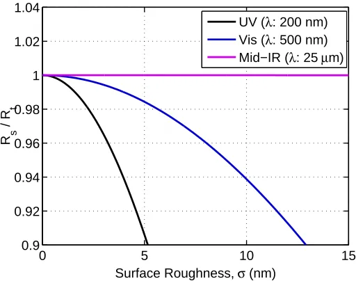
Surface roughness inherently decreases the reflectively of a mirror due to light scattering. From [22,23] this effect can be described in terms of the ratio of reflected radiant power to total incoming radiant power for a given material, as follows:
Rs Rt
=exph−(4πcosφiσ/λ)2
i
(2.2)
where Rsis the specular reflectance, Rt is the total reflectance (ie. from a perfect surface),φi is the angle of incidence,σis the RMS roughness of the surface andλis the wavelength of light under study. Figure2.1
displays the results of this relation at normal incidence (φi = 0◦) for UV, visible and Mid-IR wavelengths. Due to their short wavelengths, the specular reflectance in the UV and visible regimes are observed to be highly sensitive to surface roughness issues. This plot can be used to define the maximum surface roughness based on the desired reflectivity. For example, if a specular reflectance of 98 % is desired for visible wavelength observations, an RMS surface roughness of<6 nm is required.
0 5 10 15
0.9 0.92 0.94 0.96 0.98 1 1.02 1.04
Surface Roughness, σ (nm)
R s
/ R
t
UV (λ: 200 nm) Vis (λ: 500 nm) Mid−IR (λ: 25 µm)
2.2
Mirror Substrate
Replication techniques were chosen as the manufacturing process for the mirror substrate due to its simplicity and high manufacturing throughput. This imposes limitations on the types of materials to be used as they must be capable of being formed by molding techniques. Polymers are obvious candidate materials due to their ability to flow and conform to an underlying surface before curing. However, polymers exhibit low-stiffness and dimensional stability. A method to alleviate these issues is to implement reinforcing materials. These reinforcements can be of the particulate or fiber variety. Particulate reinforcements, such as ceramic beads or carbon nano-tubes [24], reinforce the polymer material isotropically while fibers increase stiffness primarily in one direction. However, the continuous nature of the fibers allow for a much higher increase in stiffness in comparison to dispersed particles. Multiple layers at differing fiber orientations can be used to produce a substrate with quasi-isotropic properties.
For the purposes of this study carbon-fiber reinforced polymer (CFRP) materials were implemented. Specifically, multiple plies of pre-impregnated unidirectional carbon fibers and epoxy resin are used. Thin-ply materials were selected in order to keep the substrate thin while allowing for increased design variability in laminate orientation. Two types of of carbon fibers were used for this study; T800 and M55J. A mechanical characterization of the orthotropic properties in the unidirectional state was performed for each material. The results of these studies are presented in Table 2.2. A fiber areal weight (FAW) of 17 g/m2 (gsm) corresponding to a ply thickness of ∼ 20 µm was achievable for the T800 material. This represents a reduction of 4 - 10 in the thickness of each ply in comparison to traditional CFRP materials. The M55J material had a FAW of 30 gsm and was used for the remainder of the studies as well as mirror fabrication.
Table 2.2: Material properties of unidirectional T800 and M55J carbon fibers embedded in ThinPregT M120EPHTg-1 epoxy (V
f ≈50%).
Property T800 M55J*
E1 (GPa) 128 340
E2 (GPa) 6.5 6.0
G12(GPa) 7.5 4.2
ν12 0.35 0.35
*M55J characterization courtesy of Yuchen Wei.
desired for future efforts.
To construct the mirror substrate, the laminate is laid-up initially flat and then placed atop the mandrel used for cure. The mandrel is spherical with a nominal 2.0 m ROC, thus producing nominally spherical mirror substrates. It is first treated with a release agent (Frekote 770NC) in order to prevent the part from curing to the surface. A 1/4” thick soft silicone pad is placed directly onto the backside of the laminate. This allows for an even pressure distribution to be obtained for subsequent vacuum-bagging and autoclave cure. Details of the curing process as well as process alterations implemented to mitigate post-cure shape errors are presented in Chapter4.
2.3
Reflective Front Surface
Fiber
Resin
Figure 2.2: Schematic of fiber print-through.
Figure 2.3: Schematic of resin-rich cure process used to mitigate fiber print-through.
The second method was the incorporation of a nanolaminate facesheet onto the front of the CFRP substrate. Nanolaminates are multilayer metal foils formed by sputter deposition on a precision glass man-drel [25,26]. The surface quality of the nanolaminate is dependent entirely on the roughness of the deposition mandrel and has been demonstrated down to<1 nm RMS. The bonding process is very similar to that of the resin-rich layer and is depicted in Figure2.4. A detailed overview of the nanolaminate bonding process is presented in Chapter 5. While this method still incorporates a layer of resin, the nanolaminate acts to seal the surface and therefore moisture absorption issues are not of great concern. Ultimately, this was chosen as the optimal route for mirror development due to the increase in potential surface quality. For the current effort 50µm thick nanolaminates composed of Cu and Zr layers were used. A terminal Au layer is implemented for the reflective front surface. Nanolaminates have been demonstrated on meter-scale parts and are thus scalable technologies.
Figure 2.4: Schematic of nanolaminate bonding process used to mitigate fiber print-through.
2.4
Active Layer
in various active structures. Therefore, these materials were implemented for the present study with a focus on piezoelectric ceramics. Specifically, Lead-Zirconate-Titanate (PZT) was used. The properties of this material can be found in Table2.3.
Table 2.3: Material properties for PZT-5A.
Property Value
Modulus, E (GPa) 66.0
Poisson’s Ratio,ν 0.35
Piezoelectric Constant*, d31 (pC/N) -375 Maximum Electric Field*,Emax(MV/m) 0.8 *Measured value
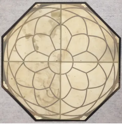
[image:29.612.206.402.450.649.2]125 µm thick flat PZT plates were used as the active elements for the mirror substrate. The plates are initially 72.5 x 72.5 mm square but trimmed to a section of an octagon using a high-speed cutting disk. The octagonal shape of the mirror also has the added benefit of accommodating identically sized plates here. The material is initially poled with continuous nickel electrodes on either side. In order to apply the custom electrode pattern, these electrodes were removed using a wet nickel-stripping agent (Caswell B-9). A materials printer (Dimatix 2800) and silver nano-particle ink (Methode 9104) was used to reprint the continuous ground plane on one side as well as the optimized pattern on the other (the pattern details can be found in Chapter7). For optimal conductivity, the ink must be sintered at 200◦C for 2 hrs. The plates are bonded to the CFRP substrate using room-temperature cure epoxy and vacuum-bagging techniques. Figure2.5displays the active layer with the custom electrode pattern on the backside of the mirror. Details of the custom electrode pattern can be found in [17,28].
2.5
Electrode Routing Layer
Due to the relatively large number of actuation channels, active mirrors often contain cluttered, bulky and massive connecting wires that can impart shape errors onto the mirror surface. This is a particular problem for the current design as the mirrors are extremely thin and thus susceptible to the mechanical constraints imposed by such wires. To alleviate this problem, conductive electrode traces are printed on a 25µm thick Kapton routing layer using the materials printer and conductive ink. Connections to the underlying electrode pads are then made using through-thickness vias and conductive epoxy. The pattern is designed to route the traces away from the active surface of the mirror to a flex-cable connector where connections to the control electronics can be made using more standard cabling techniques. The low modulus and thickness of the Kapton layer allows the mirror to remain highly flexible during actuation. Figure2.6displays the backside of a mirror after integration of the electrode routing layer.
Figure 2.6: Backside of an active CFRP mirror after electrode routing layer integration.
2.6
Mounting
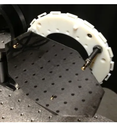
Figure 2.7: Bare CFRP substrate mounted using spherical magnets.
2.7
Overview of Fabrication Process
Figure 2.8: Overview of fabrication process.
Chapter 3
Imperfections in Symmetric Thin-Ply
Composites
3.1
Introduction
Advancements in tow-spreading techniques [29,30] have allowed for the production of extremely thin carbon fiber composite materials. The benefits of using such material have been widely studied, demonstrating an increase in mechanical performance [29, 31, 32]. The thin nature of this material also allows for the construction of extremely thin structures. Symmetric, multi-ply laminates with quasi-isotropic properties can be constructed while keeping the overall laminate thickness extremely low (< 200 µm). These thin laminates are attractive when considering lightweight shell structures for aerospace applications. In the context of replicated composite optics, this potentially enables mirror designs that can be folded into a compact initial state and then deployed upon orbit. An example of this concept is shown in Figure 3.1. However, the stringent requirements on surface accuracy remain. Therefore, it is desired to study here the post-cure shape accuracy of ultra-thin composite laminates.
3.1.1
Background
Achieving highly-accurate shapes in laminated structures is a difficult process. Significant internal stresses develop during thermal curing due to the highly orthotropic nature of the individual plies. Under uniform curing conditions and with symmetric laminates, it is predicted that the stresses will be balanced through the thickness and therefore zero out-of-plane deformations will occur. If cured on a flat surface under these ideal conditions, the laminate is expected to remain flat. However, deviations from this ideal case break the laminate symmetry, creating an imbalance in thermal stresses, ultimately resulting in post-cure shape errors. These symmetry-breaking variations can occur due to a number of factors. The first is related to variations in the homogenized properties of the plies. Several studies have been performed in order to characterize the magnitude of fiber misalignment within a ply [33, 34] and assess its effect on mechanical and thermal properties [35,36, 37, 38,39]. Errors in the through-thickness distribution of fibers within a ply have also been shown to be a factor [40]. Finally, simple variations in thickness will change the overall stiffness of each ply. These factors have the potential to produce variations within a single ply as well as between successive plies within a laminate.
Errors in the relative orientation of successive plies can also break the intended symmetry of a laminate. Hinckley [41] performed Monte Carlo analyses to assess the effect of ply misalignment on mechanical and thermal properties for various laminate orientations. Arao [42] performed a study to assess the effect of ply misalignment on the post-cured shape error of symmetric laminates. Significant twisting deformations were predicted in these studies in spite of the nominally symmetric laminate orientation. However, both of these studies were conducted for laminates constructed from relatively thick materials.
Finally, variations in the curing conditions during processing can also result in the development of shape errors. It has been shown that thermal gradients during curing can produce large out-of-plane deforma-tions [43,44].
3.1.2
Objective and Scope
The present study attempts to 1) identify the relevant imperfections associated with thin-ply fiber reinforced composites, 2) experimentally quantify the magnitude of these imperfections, and 3) assess their effect on post-cure shape errors for flat laminates.
thickness and fiber orientation are considered.
3.2
Spatially-Uniform Imperfections
3.2.1
Problem Formulation
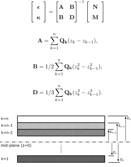
In order to identify the spatially-uniform imperfections, a study was performed using Classical Lamination Theory (CLT)[45]. CLT assumes geometric and material linearity and is used to predict the mid-plane strains and out-of-plane curvature changes of a laminate under load. The problem can be structured as follows: given a laminate constructed fromnseparate plies, the 6x6ABDstiffness matrix can be assembled relating mid-plane strains and out-of-plane curvatures,andκ, to resultant forces and moments,NandM, respectively, as follows:
κ = A B B D −1 N M (3.1) where A= n X k=1
Qk(zk−zk−1), (3.2)
B= 1/2 n
X
k=1
Qk(z2k−z 2
k−1), (3.3)
D= 1/3 n
X
k=1
[image:35.612.189.416.271.560.2]Qk(zk3−zk3−1). (3.4)
Figure 3.2: Through-thickness coordinate definition for Classical Lamination Theory.
Qkis the orthotropic stiffness matrix of thekthply in the laminate coordinate system (x/y) andzk is the through-thickness interface coordinate of that ply and its neighbor, as shown in Figure3.2. Qkis dependent on the material properties of the kth ply, as well as the orientation of the ply with respect to the global coordinate system. For each ply it is defined as
Qk= [T]−1k [QPMCk ][T] −T
where QPMCk is the stiffness matrix of the kth ply in the prime material coordinate (PMC) system. The PMC system is aligned parallel and perpendicular to the nominal fiber direction for this study. [T]k is a rotation matrix dependent on the ply orientation and is defined as
[T]k =
c2 s2 2cs
s2 c2 −2cs
−cs cs c2−s2
(3.6) with
s=sin(θk), (3.7)
c=cos(θk), (3.8)
whereθk is the orientation of the kthply with respect to the global reference frame (about the z-axis). For the present study the mid-plane strains and out-of-plane curvatures produced after the laminate has been cured and returned to room-temperature are of interest. These are produced as a result of the internal thermal stresses developed during cure. These stresses can be expressed as resultant thermal forces and moments,NThermal andMThermal, respectively, as follows:
NThermal =
n
X
k=1
Z zk
zk−1
Qkαk∆T dz, (3.9)
MThermal=
n
X
k=1
Z zk
zk−1
Qkαk∆T zdz, (3.10)
whereαkis an array of in-plane thermal expansion coefficients for thekthmaterial and ∆T is the temperature change experienced during cooling. αkalso depends on the orientation of the fibers within a ply and is defined as
αk= [R][T]−1[R]−1[αPMCk ], (3.11)
where αPMC
k is the array of thermal expansion coefficients for thekth layer in the PMC system and R= diag{1, 1, 2}.
Therefore, Equation 3.1becomes
κ = A B B D −1 NThermal MThermal (3.12)
and the out-of-plane curvatures produced during cure can be predicted.
unstressed state after the completion of the cure. Second, after this process the material is linear elastic with properties independent of temperature. Third, the laminate is unconstrained and therefore free to deform during cooling. These assumptions are known to be partially invalid in a practical setting. However, they allow for an initial investigation into the thermal deformations produced during cure.
3.2.1.1 Identification of Relevant Parameters
Using the formulation above, the conditions required to ensure out-of-plane curvature changes do not arise during cooling can be identified. Firstly, it is observed through Equation 3.9 that upon integration, the resultant thermal forces are always non-zero during cool-down. Therefore, from Equation3.1theBmatrix must be null and thus no coupling between out-of-plane curvatures,κ, and resultant thermal forces,Nthermal, must exist. The first condition required for this to be satisfied is that plies opposite one another from the neutral axis must have identical thicknesses,tk. This can be expressed as
tk=t[n−(k−1)], (3.13)
with k=1, 2, ..., n/2 for a laminate with an even ply count. The second condition is that opposing plies must possess identical stiffness matrices, Qk. From Equations 3.5 and 3.6, this requirement reduces to a constraint on the ply orientation,θk(assuming identical properties in the PMC reference frame). Therefore
θk=θ[n−(k−1)]. (3.14)
.
Additionally, asDis never null for practical laminates there must be zero thermal moments, Mthermal, developed during cure. From Equation3.10it can be deduced that this condition is satisfied if perfectly sym-metric lamination conditions exist and the laminate undergoes a uniform temperature change during cooling. Namely, opposing plies must have identical mechanical and thermal properties (QPMCk , αPMCk ), fiber ori-entation, θk, equal thicknesses, tk, and ∆T must not be a function of the through-thickness coordinate. Therefore,
∆T6= ∆T(z). (3.15)
.
Table 3.1: Orthotropic properties of unidirectional T800 carbon fibers embedded in ThinPregT M 120EPHTg-1 epoxy (Vf ≈60%).
Property Value
E1(GPa) 127.9
E2(GPa) 6.5
G12 (GPa) 7.5
ν12 0.35
α1 (ppm/◦C) 0.0
α2 (ppm/◦C) 20.0
3.2.2
Characterization of Spatially-Invariant Imperfections
This section outlines the procedures used to experimentally characterize the imperfections mentioned above. To do so, 100 mm square laminate coupons were constructed. Symmetric 4-ply, [0◦/90◦]sflat laminates were used for this study as they are the thinnest symmetric laminates possible. The coupons were constructed from material comprised of T800 fibers embedded in an epoxy matrix. The material was in an initial prepreg form with a resin content of 38% by weight and each ply had a fiber areal weight (FAW) of 17gsm. The coupons were laminated and cured atop a flat glass plate. A compliant silicone backing pad was used to provide an even pressure distribution during cure. The laminates were vacuum bagged and autoclave cured at a temperature of 120◦C for 2 hours and under an external pressure of 80 psi. The rate of loading and unloading were 2 ◦C/min and 3 psi/min for the temperature and pressure profiles, respectively. The mechanical and thermal (CTE) properties of the T800 material were measured experimentally prior to the study and are listed in Table3.1.
3.2.2.1 Thickness Variations
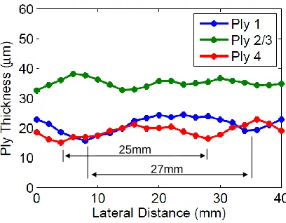
Ply thickness measurements were made using micrographs of the laminate cross-section and calibrated ob-jective lenses. Images were captured using a Nikon LV-150 microscope. Specimens were first cross-sected and potted in clear casting epoxy. Once cured, the specimens were lapped down using a series of grinding wheels and polished to the desired surface finish for imaging. This allowed the plies as well as individual fibers to be imaged.
Figure 3.3: Micrograph of laminate cross-section displaying ply thickness measurements.
Table 3.2: Ply thickness measurements.
Ply Mean Thickness (µm) Std. Dev. Thickness (µm)
1 21.1 2.6
2/3 17.8 2.0
4 19.8 2.2
Avg 19.6 2.3
3.2.2.2 Ply Misalignments
Measurements of the ply orientations were performed using optical techniques as well. An existing 8-ply [0◦/45◦/-45◦/90◦]s laminate was used for this study as the higher number of plies allowed for increased measurements. In order to measure the relative angle of the successive plies it was necessary to expose the inner plies for imaging. To do so, sections of the laminate were polished down in the through-thickness direction at depths corresponding to the various ply interfaces, as shown in Figure3.4. Multiple images of the now exposed plies, and fibers within, were captured while keeping the specimen fixed to the translation stage.
+45o -45o 90o
0o
Ply 1 Ply 2 Ply 3 Ply 4
x y
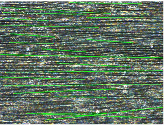
A Nikon ShuttlePix P-400R digital microscope at 400x total magnification (800 µm field of view) was used to capture images of the plies. The larger field of view was necessary to take fiber angle measurements over longer length scales. The specimen was fixed to a precision XY translation stage, allowing images to be captured at various in-plane locations while maintaining a common reference frame. The orientation of individual fibers within each image were measured using a line-detecting algorithm and custom Matlab script. The algorithm used was a Hough Transform [46], a classic method of detecting features within an image. A total of 250 - 270 fiber angle measurements were performed from 15 images captured at each ply depth. Figure3.5 displays an image of the fibers along with the line-detection produced using the Hough Transform.
Figure 3.5: Image of line detection algorithm used to perform fiber measurements.
Figure 3.6 displays the measured fiber distributions for each ply along with the mean and standard deviations in fiber angle. It can be seen that the measured fiber angles follow an approximate normal distribution for each ply. As the global reference frame was kept fixed during imaging, the mean fiber orientation of each ply can be compared to the intended laminate orientation, providing an assessment on the accuracy to which the plies have been aligned. As shown in Figure3.6it was found that each of the plies were oriented to an accuracy of approximately 0.3◦. Therefore it is assumed that this level of misalignment is present for all plies.
3.2.2.3 Thermal Gradients During Cure
−100 0 10 10 20 30 40 50
0°(ref), σ: 1.9°
Fiber Angle (deg)
−50 −40 0 10 20 30 40 50
−44.7°, σ: 1.9°
Fiber Angle (deg)
40 50 0 10 20 30 40 50
45.3°, σ: 2.2°
Fiber Angle (deg)
80 90 100
0 10 20 30 40 50
90.2°, σ: 2.2°
Fiber Angle (deg)
Figure 3.6: Fiber angle measurements of external and internal plies used to assess ply alignment accuracy.
displays the thermal profile during cure with a detailed view of the constant-temperature “soak” section. A maximum through-thickness temperature change of approximately 0.5◦C was measured. The temperature is kept relatively constant throughout this section, with only slight variations observed due to the autoclave control cycle (high-frequency variations are attributed to thermocouple noise). From this study it is apparent that the mandrel-side of the part is at a higher temperature for both thermocouple locations. Due to this increased cure temperature, the mandrel-side of the part will be subject to a higher degree of cooling once the part is brought back down to room temperature. An in-plane temperature variation of approximately 1◦C was measured across the surface of the laminate.
3.2.3
Numerical Modeling
While the CLT analysis is useful in identifying relevant parameters causing shape errors, it is limited by the assumption of geometric linearity. This is especially true for very thin laminates, as deflections much greater than the thickness are expected. Therefore, a finite element model was developed to investigate the effect of the above imperfections on post-cure shape errors. The commercial package, Abaqus Standard/CAE 6.12 [47], was implemented with S4R elastic shell elements. The orthotropic material properties of the T800 material outlined in Table3.1were defined as the nominal properties of each ply. The laminate orientation was defined using the built-in composite stack lay-up feature. The laminate was modeled as a 4-ply, [0◦/90◦]s, 250 mm square flat plate constrained at a single node in all 6 degrees of freedom at the center of the plate. Each ply was assigned a nominal thickness of 20µm. An element size of 2.5 mm was used resulting in 10,000 total elements across the laminate.
(a)
[image:42.612.172.432.223.518.2](b)
made.
3.2.3.1 Uniform Variations in Ply Thickness
Figure3.8 displays the resulting curvature changes,κx, κy, andκxy, and RMS shape error due to uniform changes in ply thickness. This was performed by varying the thickness of the top 0◦ ply while keeping all others fixed. It was assumed that the material properties of that ply remained constant throughout this process.
As evident in Figure 3.8(a), extremely large curvatures arise due to small changes in ply thickness. The dominating curvature change occurs in the y-direction, resulting in the laminate taking on a cylindrical mode of deformation. The CLT prediction of κy agrees well with that obtained through the non-linear study. However, a small component of κx is predicted in addition to the dominating κy not found in the non-linear analysis. From Figure 3.8(b), it can be seen that extremely large shape error magnitudes form over the 250 mm square plate due to small changes in ply thickness. (Note: uniform thickness changes in the internal 90◦ plies do not result in curvature changes as the laminate remains balanced).
0 0.2 0.4 0.6 0.8 1 −0.5 −0.4 −0.3 −0.2 −0.1 0 0.1 0.2 0.3
Variation in Ply Thickness (µm)
Curvature (m −1 ) Kx Ky Kxy (a)
0 0.2 0.4 0.6 0.8 1 0 200 400 600 800 1000 1200 1400
Variation in Ply Thickness (µm)
RMS Error (
µ
m)
NL FEM CLT
(b)
Figure 3.8: Results of NL FEA (solid) and CLT prediction (dashed) for uniform variations in ply thickness. a) Laminate curvatures and b) resulting shape error magnitudes.
3.2.3.2 Variations in Ply Alignment
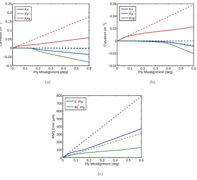
The effect of ply misalignments on the post-cured shape of the laminate was studied next. To model this effect, the mean orientation of a single ply was varied in the laminate orientation while keeping all others fixed. Figures 3.9(a) and3.9(b) display the resulting curvature changes as a function of ply misalignment in the terminal 0◦ and internal 90◦ plies, respectively. Figure3.9(c)displays the corresponding RMS shape error.
for the 90◦ ply, as the resulting curvatures are of higher magnitude. This is as expected as the 0◦ ply is further from the neutral axis of the laminate, thus producing a larger thermally-induced moment from the imbalance. Secondly, for both the 0◦ and 90◦ plies, and at small values of ply misalignment, there is good agreement between the results of the non-linear finite element analysis and CLT prediction. At this point, both analyses predict a strong saddle/astigmatic shape, asκxyis the only non-zero curvature component. As the magnitude of ply misalignment is increased, the non-linear results deviate from the CLT prediction and the rate of growth ofκxy declines. Upon further increase of the ply misalignment, the non-linear analysis captures a mode change in the deformation of the laminate as κx and κy become non-zero. This point occurs at a misalignment of approximately 0.15◦for the 0◦ply and 0.3◦for the 90◦ ply. Finally, by studying Figure3.9(c) it can be seen that significant magnitudes of shape errors arise from small ply misalignments. It is also apparent that the CLT analysis greatly over-predicts the magnitude of shape error during cooling.
0 0.1 0.2 0.3 0.4 0.5 0.6 −0.1 −0.05 0 0.05 0.1 0.15 0.2 0.25
Ply Misalignment (deg)
Curvature (m −1 ) Kx Ky Kxy (a)
0 0.1 0.2 0.3 0.4 0.5 0.6 −0.04 −0.02 0 0.02 0.04 0.06
Ply Misalignment (deg)
Curvature (m −1 ) Kx Ky Kxy (b)
0 0.1 0.2 0.3 0.4 0.5 0.6 0 100 200 300 400 500 600 700 800
Ply Misalignment (deg)
RMS Error (
µ
m)
0° Ply 90° Ply
[image:44.612.108.494.285.638.2](c)
3.2.3.3 Thermal Gradients
Finally, the effect of thermal gradients during cure was studied. The temperature change of the shell mid-plane was set to the nominal value of -100 ◦C as before; however, a linear variation through the thickness was also defined. Figure 3.10 displays the resulting deformation due to a through-thickness change in temperature. It can be seen that this produces a cylindrical deformation oriented in the y-direction asκy is the dominating curvature term. The results of the CLT analysis agree well with that of the non-linear study, as evident by Figure3.10(b).
0 0.2 0.4 0.6 0.8 1 −0.14 −0.12 −0.1 −0.08 −0.06 −0.04 −0.02 0 0.02
Through−Thickness Temperature Change (°C)
Curvature (m −1 ) Kx Ky Kxy (a)
0 0.2 0.4 0.6 0.8 1 0
50 100 150 200
Through−Thickness Temperature Change (°C)
RMS Error (
µ
m)
NL FEM CLT
(b)
Figure 3.10: Results of NL FEA (solid) and CLT prediction (dashed) for thermal gradients during cure. a) Laminate curvatures and b) resulting shape error magnitudes.
3.2.3.4 Sensitivity Analysis
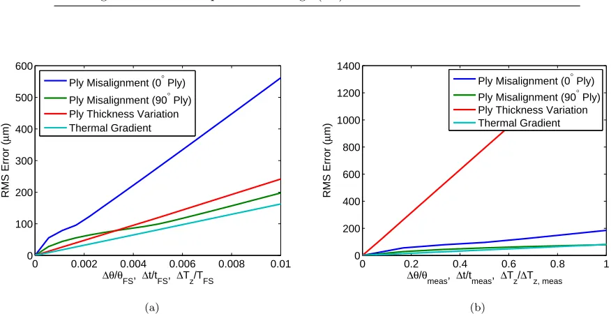
In order to compare the relative effect of each imperfection, it was necessary to normalize the magnitude of each. Two methods of normalization were considered: normalization by the full-scale value of imperfection and normalization by the measured values presented in Section 3.2.2. The full-scale values were taken to be 1) the difference between the terminal/internal ply orientations, 2) the total ply thickness, and 3) the full temperature change experienced during cure. The measured values were defined as 1) the maximum deviation in measured ply orientation, 2) the difference in thickness between the top and bottom plies, and 3) the through-thickness difference in temperature measured during cure. Table 3.3 lists these values for each imperfection.
Figure 3.11(b) displays the influence of each imperfection as a fraction of their measured values. This analysis provides insight into the level of shape error reduction that can be achieved if the magnitude of imperfections were to decrease from the current measured values. From this analysis it can be seen that the variation in ply thickness is clearly the dominant factor. The deformation of the laminate is extremely sensitive to variations in this parameter with out-of-plane deformations in excess of 1500µm RMS.
Table 3.3: Full-scale and standard deviations of imperfections.
Imperfection Full-Scale Value Measured Value
Ply Misalignment (deg) 90.0 0.3
Ply Thickness Variation (µm) 20.0 1.3
Through-Thickness Temperature Change (◦C) 100.0 0.5
0 0.002 0.004 0.006 0.008 0.01
0 100 200 300 400 500 600
∆θ/θFS, ∆t/tFS, ∆Tz/TFS
RMS Error (
µ
m)
Ply Misalignment (0° Ply)
Ply Misalignment (90° Ply) Ply Thickness Variation Thermal Gradient
(a)
0 0.2 0.4 0.6 0.8 1
0 200 400 600 800 1000 1200 1400
∆θ/θmeas, ∆t/tmeas, ∆Tz/∆Tz, meas
RMS Error (
µ
m)
Ply Misalignment (0° Ply) Ply Misalignment (90° Ply) Ply Thickness Variation Thermal Gradient
[image:46.612.77.515.261.486.2](b)
Figure 3.11: RMS error as a function of imperfection magnitude. Results are normalized by a) the full-scale (FS) values and b) the measured (meas) values in Table3.3.
3.2.4
Shape Error Measurements
susceptible to gravity effects.
Figure3.12displays the measured shapes of the 4-ply laminates. It is apparent that there are significant post-cure shape errors present. The errors are dominated by cylindrical modes oriented in the y-direction and have a peak-to-valley amplitude of approximately 6.0 mm (1.07 - 1.41 mm RMS). There is also a slight twisting mode associated with each sample.
Spec. 1
Spec. 2
Spec. 3
RMS: 1.07 mm RMS: 1.16 mm RMS: 1.41 mm Z (mm)
X (mm)
Y
(
mm)
X (mm)
Y
(
mm)
X (mm)
Y
(
mm)
Z (mm) Z (mm)
Figure 3.12: Measured shape errors of the three constructed laminates. <