Mitigating supply and production uncertainties with dynamic scheduling using real-time transport information

Version: Accepted Version

Article:

Mogre, R, Wong, CY and Lalwani, CS (2014) Mitigating supply and production

uncertainties with dynamic scheduling using real-time transport information. International

Journal of Production Research, 52 (17). 5223 - 5235. ISSN 0020-7543

https://doi.org/10.1080/00207543.2014.900201

[email protected] https://eprints.whiterose.ac.uk/

Reuse

Unless indicated otherwise, fulltext items are protected by copyright with all rights reserved. The copyright exception in section 29 of the Copyright, Designs and Patents Act 1988 allows the making of a single copy solely for the purpose of non-commercial research or private study within the limits of fair dealing. The publisher or other rights-holder may allow further reproduction and re-use of this version - refer to the White Rose Research Online record for this item. Where records identify the publisher as the copyright holder, users can verify any specific terms of use on the publisher’s website.

Takedown

If you consider content in White Rose Research Online to be in breach of UK law, please notify us by

RESEARCH ARTICLE

Mitigating supply and production uncertainties with

dynamic scheduling using real-time transport information

Riccardo Mogrea ∗ _{Chee Y. Wong}b _{and Chandra S. Lalwani}a

a_{Hull University Business School, University of Hull, Kingston upon Hull, UK.;} a_{Leeds University Business School, University of Leeds, Leeds, UK.}

(February 4, 2014)

Supply and production uncertainties can affect the scheduling and inventory performance of final production systems. Facing such uncertainties, production managers normally choose to maintain the original production schedule, or fol-low the first-in-first-out policy. This paper develops a new, dynamic algorithm policy that considers scheduling and inventory problems, by taking advantage of real-time shipping information enabled by today’s advanced technology. Sim-ulation models based on the industrial example of a chemical company and the Taguchi’s method are used to test these three policies under 81 experiments with varying supply and production lead times and uncertainties. Simulation results show that the proposed dynamic algorithm outperforms the other two policies for supply chain cost. Results from Taguchi’s method show that com-panies should focus their long-term effort on the reduction of supply lead times, which positively affects the mitigation of supply uncertainty.

Keywords:Simulation; supply uncertainty; production uncertainty; dynamic scheduling; information sharing.

1. Introduction

Demand, production and supply uncertainties can importantly affect the performance of final production systems (Sunet al., 2012). Operationally, demand is stable because production requirements are defined by the master production schedule, with supply and production constituting the primary sources of uncertainties (Kim and Springer, 2008 and Songet al., 2014).

Their influence could be mostly measured by delays in supply and production lead times. Operational uncertainties in supply include transport time variability, quantity

∗_{Corresponding author. Email: [email protected]}

ISSN: 1478-6451 print/ISSN 1478-646X online ©2012 Taylor & Francis

inaccuracies and supplies not meeting the specifications (Zsidisin, 2003 and Ghadge et al., 2012)). The two latter uncertainties require the supplier to redeliver the items, caus-ing further disruptions to supply lead times. Natural hazards could also disrupt supply operations (Pawar and Rogers, 2013): because of the 2011 Thailand floods the global magnetic-hard-drive supply was delayed by several weeks (Arthur, 2011). Operational uncertainties in production include glitches, malfunctions, congestions and lack of con-trol (Tomlin, 2006 and Micheliet al., 2014). The two latter uncertainties directly disrupt production lead times. The two former uncertainties require reworks. Those in turn delay production operations.

In particular, the effects of supply-side transport disruptions could be severe in just-in-time settings, for example, the supply of automotive components or perishable food or chemical raw materials. Although disruptions and delays in production could be timely identified, it was not so for transport operations until recently, thanks to technology developments such as GPS-based vehicle tracking (Gaukleret al., 2008). Allowing real-time gathering of shipment status, these technologies have attracted some attention from practitioners as they could be used to dynamically reschedule production if supply-side transport disruptions occur (GIS Park, 2011). However, it is unclear how such applica-tions would work and what is the entity of the benefits ensuing from their introduction. To address this relevant practical problem we propose a GPS-based technology ap-plication and develop a heuristic algorithm, called ‘Dynamic algorithm’ to re-schedule production according to real-time transport information that we compare by a simulation study against commonly used scheduling policies.

The setting, the assumptions and the data of the simulation study are based on a chem-ical plant producing calcium carbonate.The plant is managed by a Swiss-based chemchem-ical company with worldwide presence, specialised in the production and distribution of in-dustrial minerals. We use the pseudonym ‘Carb.Co.’ when we refer to the company to preserve its anonymity.

This paper could be classified among those academic studies considering demand, sup-ply or production uncertainties in final production systems. We contribute to filling the gaps in that academic literature in the following ways. First, our study considers sup-ply and production uncertainties, although previous literature seldom considers these uncertainties simultaneously. Second, to mitigate delays and congestions in the produc-tion system, our algorithm considers scheduling and inventory decisions. Again, although these decisions are strongly inter-related, previous literature rarely consider scheduling and inventory policies together.

A more theoretical contribution of this work is related to how to calculate inventories between known demand and uncertain supply lead times when these are lognormally distributed. The choice of such distribution is motivated by empirical evidence collected from the industrial example and confirmed by its suitability to capture lead time vari-ability (Bakshiet al., 2011).

tracking in supply chains, with Gaukleret al.(2008) focusing on the process of expediting late orders and Sari (2010) conducting his study in a multi-echelon setting. Both studies show that the benefits ensuing from tracking technologies are often intangible, for supply chain visibility, and, therefore, difficult to evaluate. Ballest´ın et al., 2013 looked at the role of RFID in sequencing warehouse operations. They compare, as we do, static policies and technology-based dynamic polices.

Although the setting of the problem studied here is new, we can still relate our work to previous papers in the scheduling and inventory management literature, especially to those studies considering uncertainties in final production systems. These can be divided into four categories: (1) papers calculating safety lead times, (2) papers analysing the economic lot-scheduling problem, (3) papers modelling the restoration of a disrupted schedule and (4) papers identifying and testing dynamic scheduling rules.

The first category of papers studies re-ordering policies for single-product assembly sys-tems with deterministic demand and independent and identically distributed component lead times. Cost-minimising policies are usually formulated for safety lead times, defined as the difference between the planned and expected lead times. Tang and Grubbstr¨om (2003) obtain results for the continuous time setting. Louly et al. (2008) extended the model of Tang and Grubbstr¨om (2003) to a discrete time environment, by also allowing more components. Loulyet al.(2008) further allowed the values of component lead times to be generated by various probability distributions. These papers connect to our study because they also assume deterministic demand and try to identify inventory policies to hedge against supply lead times uncertainty. They study a more complicated inventory setting than us in which each product is assembled from several components. On the other side, their study is simpler in other dimensions: they do not consider production uncertainty and scheduling policies.

The second group of papers aims at finding cyclic schedules for manufacturing various products with the goal of minimising holding and setup costs. These studies are similar to the present work in their objective to consider inventory and scheduling decisions when managing final production systems. Contrary to the present paper, these studies analyse inventory and scheduling decisions jointly and not sequentially as we do here. However, they do not consider production and supply uncertainties, with only few studies considering demand variability (Leachman and Gascon, 1988 and Gallego, 1990).More recently, Wanget al., 2012 analysed the extension of this problem to a dynamic control setting.

share a set of resources. Moreover, they do not consider inventory decisions and supply uncertainties.

The final group of papers proposes and tests dynamic scheduling rules in final pro-duction systems. All these contributions consider processing time uncertainty but not supply lead time variability. This category of papers is related to our study because they propose heuristic dynamic scheduling rules as we do here. Dynamic rules require the knowledge of many events occurring in the production system leading to large state spaces. Additionally, decisions in dynamic rules are made in discrete time. For these rea-sons, analytical approaches are often difficult to accomplish and the studies in this last group rely on simulation to test the rules proposed. Hausman and Scudder (1982) pro-posed a model in which dynamic policies provided an important reduction in spare parts inventory compared with static policies for an assembly job-shop processing various jobs on several machines. Wein and Ou (1991) tested how the adoption of various schedul-ing policies affects the flow time of an assembly system similar to the one described by Hausman and Scudder (1982). More recently, Gonget al.(2011) tested the effectiveness of a dynamic rule called ‘distributed arrival time control’ to schedule jobs in assembly lines and assembly cells. The results indicated assembly cells outperform assembly lines with specific reference to an indicator associated with the due-date variation of jobs.

3. Problem description and innovative application

3.1. Problem description

The supply chain studied and the assumptions of the model are based on the indus-trial example of Carb.Co., a producer of calcium carbonate interested in synchronising its production process with information about inbound supply shipments. Drivers could already use smartphones to update the company about inbound shipments’ status. How-ever, Carb.Co. was interested in automating the tracking to make updates more frequent and regular. Based on this need, we propose the innovative application described in¶3.2. The plant under consideration entails a single multi-product production line receiv-ing chemical raw materials from various suppliers. The production line makes various products from raw materials according to a predetermined and fixed daily production plan, which follows the expected raw-material arrival times. Each raw material is sent to the production line independently by road and is transported by a third-party logistics provider. We assume the supply shipment ready-time to be reliable but the transport lead time can be variable. Moreover, we assume production lead times to be random as they directly depend on the variable raw-material quality.

Inventory holding costs are charged per raw material and per time unit, also for those goods in transit. When a raw material necessary to make the product scheduled next for assembly has not yet arrived or is not in stock, it is necessary to decide whether to wait for the raw material to arrive or to schedule a later production.

The decision horizon is constituted by a single working day. If everything goes smoothly, the production is completed in the regular time. However, with delays, managers can recur to an overtime shift at a cost to ensure that all the products are manufactured. If some products cannot be produced even in the time slot allotted to overtime, a penalty cost per product is charged.

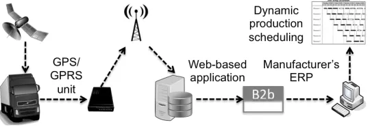
Figure 1.: The proposed technological application.

Changeover times imply delays in the production schedule that may require using over-time at additional cost, or may even result in the non-completion of the production of raw materials in the given horizon. Note that changeover times are only associated with schedule changes, and are not related to setup times, included in the processing times. We assume changeover times and costs to be independent from the sequence.

Managers define the original production schedule based on structured techniques, which consider constraints such as the capacity of the plant and the product due dates. To mitigate supply and production uncertainties in the short time horizon, the managers may choose to follow the original production schedule, named ‘No changes’, or always produce the first raw material arrived, called FIFO. ‘No changes’ and FIFO policies do not include inventory decisions. These two policies are commonly used in practice, primarily because of the lack of real-time information.

3.2. Innovative application and ‘Dynamic algorithm’

We propose a technological application that can be introduced in the setting described in

¶3.1 to trace shipment status and to allow the manufacturer to make dynamic informed decisions about its production schedule (Figure 1). Lorries are traced real-time by the 3PL through automated GPS/GPRS units. The route leading from each supplier to the manufacturer is divided into road-segments, each taking the same average lead time. Through a technique called geo-fencing, the GPS technology tracks when a lorry enters or exits a specific road segment. This information is in turn transmitted to the 3PL’s in-formation systems through GPRS cellular technologies. An e-commerce B2b application, such as a traditional EDI connection or a web-EDI connection, is used to send shipment information from the 3PL to the company’s ERP system, which makes a dynamic sched-ule update possible. Given the updated location information of each lorry, it is possible for the company to forecast the arrival of each raw material in real-time. Combined with the availability information of stocks of raw materials on hand, the company may decide to dynamically change the schedule of the products after our proposed algorithm.

of long lead times (Bakshi et al., 2011). The stock allocation rule of our static policy is encapsulated in Proposition 3.1.

Proposition 3.1 : The demand of a raw material is constant and unitary. Its supply lead time is modelled after the sequence of X1. . . Xk iid lognormal variables with mean

µx and standard deviation σx for i= 1. . . K. Define the customer service level CSL of

the supply as the probability of a raw material arriving before a particular time threshold t, after which the manufacturer’s operations may be disrupted. Then the condition for assigning a stock unit can be written as follows:

exp(F−1

Y (CSL, µy, σy)−µx ≥t (1)

The term on the left of the inequality can be interpreted as the expected delay, with µx

the mean of the compound lognormal variableX obtained through the Fenton-Wilkinson approximation andF−1

Y the distribution of the normal variableY derived from X.

The proof of Proposition 3.1 can be found in Appendix A.

The ‘Dynamic algorithm’ is described as unified modelling language activity diagram in Figure 2. Although the shipment is updated after every route segment, the algorithm computes the expected time of arrival of each raw material based on 1) the current segment where the raw material is and 2) the information about the lognormal variables. The algorithm further considers the changeover time tc, namely, the time needed to set

up the assembly line in case the production sequence is changed. Timetc minutes before

the line is available for production, all the raw materials arrived or due to arrive in the nexttc minutes are possible candidates for production next. The next raw material

to be manufactured among those arriving or arrived is chosen because of the original production schedule, to avoid the changeover cost. This choice may not be possible, for instance, when the raw material originally scheduled next for production has not yet arrived or is not expected to be arriving intcminutes and at least one other raw material

has arrived or is arriving in tc minutes. In this latter case the production sequence is

changed and a changeover cost is charged. Once the algorithm effectively schedules a product to be manufactured next, the line is made unavailable for the other products. Once the raw material scheduled for production has arrived and once the line is available, the production starts.

4. Simulation

4.1. Simulation model

We developed a discrete event simulation model using the language SIMAN and its visual interface Arena 13.0 to compare the effectiveness of the ‘Dynamic algorithm’ against ‘no changes’ and FIFO policies. We chose to use a simulation approach because the problem has not been considered tractable analytically for the following reasons: 1) the large state space necessary to the ‘Dynamic algorithm’ to make the decisions and 2) the scheduling rules are triggered by discrete events such as the arrival of raw materials and the final production line becoming available for manufacturing.

Figure 2.: The proposed ‘Dynamic algorithm’.

real-data from the industrial example, some of which have been scaled. A panel consisting of one academic and one practitioner has verified and validated the simulation model.

The model incorporates ten sub-models developed for each raw material shipped to the assembly line by the ten suppliers. Each sub-model is associated with a physical compo-nent, replicating transport and production activities, and a decision-making compocompo-nent, changing because of the algorithm used.

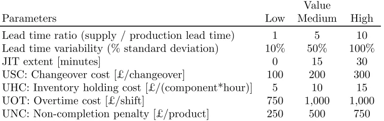
Lead time ratio (supply / production lead time) 1 5 10 Lead time variability (% standard deviation) 10% 50% 100%

JIT extent [minutes] 0 15 30

USC: Changeover cost [£/changeover] 100 200 300 UHC: Inventory holding cost [£/(component*hour)] 5 10 15

UOT: Overtime cost [£/shift] 750 1,000 1,000

UNC: Non-completion penalty [£/product] 250 500 750

Table I.: Cost, lead times and just-in-time parameters.

required sequence of production, the average production lead times and the hours of operation of the plant. A delivery plan is created based on the production plan depending on the time lag between the expected raw-material arrival and the start of the production, called just-in-time extent or JIT. The planned shipping times of all raw materials are calculated based on the average supply lead times and planned production times. In our simulation, the shipping times equal the arrivals of entities, the raw materials, into the system.

The final production is modelled based on two normal shifts of six hours each. Addi-tional overtime of six hours is available if raw materials cannot be produced, because of delays during regular work hours. We determinedCSLbeing 80% andtbeing two hours of delays. The changeover time ortc is set to 30 minutes, and three simulation files are

used with one each for ‘No changes’, FIFO and ‘Dynamic algorithm’ policies.

Table I shows relevant parameters and costs used in the model. The lead time ratio con-veys the magnitude of supply lead times compared with production lead times. Olhager (2003) uses the multiplicative inverse of this ratio to position the order penetration point in a supply chain. Higher values of this ratio mean longer supply lead times, expected to amplify delays and congestions because of supply variability. The lead time variability is measured as the relative standard deviation of lead times. This measure is easy to com-pute from historical data and commonly used in operations management literature. As described previously, the JIT extent is the scheduled slack between the expected arrival time of raw materials in the plant and the expected start of production in which those materials will be employed. Lower values of this indicator convey the intuitive idea that the JIT process is tighter.

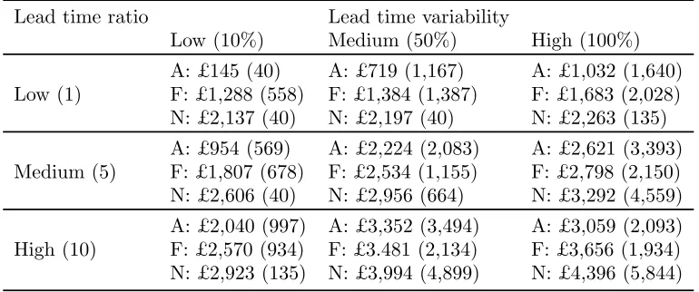
A:£2,040 (997) A:£3,352 (3,494) A: £3,059 (2,093) High (10) F: £2,570 (934) F:£3.481 (2,134) F: £3,656 (1,934) N:£2,923 (135) N:£3,994 (4,899) N: £4,396 (5,844)

Table II.: Selection of simulation results, with the number of runs in brackets (A, F and N mean ‘Dynamic algorithm’, FIFO and ‘No changes’, respectively).

4.2. Simulation results

We tested the three policies using the medium values of the unit costs and under the low, medium and high values of three variables: supply lead time variability, ratio between supply and production mean lead times and just-in-time extent, leading to 81 exper-iments. Because we found that the JIT extent has a modest influence on the cost, for clarity we show the results with JIT extent equal to 15 minutes (Table II). The number of replications or simulation runs for each experiment varies because it is calculated based on 5% confidence interval with the indifference zone set to 50 cost units, according to the Dudewicz and Dalal method (Law, 2006, Chapter 10). A unit cost of 50 is chosen because such daily saving would not justify the introduction of the real-time technology necessary to adopt the ‘Dynamic algorithm’. Fewer runs are required for experiments with lower lead time variability and a higher ratio between supply and production lead time.

The simulation results suggest that the ‘Dynamic algorithm’ is the most effective policy. ‘No changes’ is always the most expensive solution as waiting for a delayed predetermined raw material increases holding, overtime and non-completion costs.

For higher values of the ratio between supply and production lead time the cost is higher. Moreover, the cost increases when the supply lead time variability increases for almost every experiment. This effect is principally relevant to high values of the ratio between supply and production lead time. Because lead time variability is calculated as a percentage of the supply lead times longer lead times imply higher variability.

We use Figure 3 to illustrate further results. The ‘Dynamic algorithm’ seems to work principally well in two settings: for low levels and for high levels of lead time variability. For low levels of lead time variability the scheduling rule based on both the components having arrived and due to arrive is principally effective. FIFO performs worst as this policy is too myopic and will always schedule the first raw material arriving, with high chance of scheduling the ‘wrong product’ and ensuing high changeover costs. For high levels of lead time variability the inventory policy allocates initial stock of those raw ma-terials characterised by high variability. This rule reduces overtime and non-completion costs that could have been caused by the possible delays in the shipments of these raw materials.

Figure 3.: Illustration of the simulation results.

time ratio, when the supply lead time variability increases from ‘medium’ to ‘high’ the cost of ‘Dynamic algorithm’ decreases, because the ‘Dynamic algorithm’ stock alloca-tion mechanism works principally well for high supply lead time and high variability, as mentioned earlier. Furthermore, the ‘Dynamic algorithm’ performs less satisfactorily compared with the FIFO policy when the ratio between lead times is high under medium lead time variability and high JIT extent. The ‘Dynamic algorithm’ and FIFO have simi-lar performance in experiments characterised by intermediate variability, especially when the ratio between supply and production mean lead times is high. Nevertheless, it is nec-essary to consider that the parameters behind stock allocation, namely, the threshold and the customer service level, have been selected for the ‘Dynamic Algorithm’ to perform well in various experiments, namely, with variability ranging from 0.1 to 1.0. We expect, in the real world, companies will face a narrower range of variability. Therefore, the two parameters associated with initial stock allocation could be refined for the ‘Dynamic Algorithm’ to perform well also in case the standard deviation of the variability is 0.5 of the mean supply lead times.

Therefore, if compared with FIFO, the ‘Dynamic algorithm’ has higher holding costs, which nevertheless lead in most cases to lower supply chain cost.The effects of lead time ratio on costs allows to gain further understanding of the stock allocation mechanism used in the ‘Dynamic algorithm’. If the lead time variability is low, delays in transport are limited and its real-time scheduling logic avoids unnecessary changeovers by waiting for components due to arrive soon. If the lead time variability is high, delay-critical compo-nents are assigned in stock before the simulation starts. This preventive stock-allocation increases holding costs, but decongests the system, allowing larger savings in changeover, overtime and non-completion costs. Medium lead time variability systems are more con-gested than high lead time variability systems because their variability is not so high to trigger initial stock allocations. However, the entity of delays could still be important especially when lead time ratios are medium or high. In these settings, changeover costs grow, making the ‘Dynamic Algorithm’ similar to FIFO for the supply chain cost. As stated above, companies facing medium lead time variability need to fine-tune the initial stock allocation of the ‘Dynamic Algorithm’ to enhance its performance over FIFO.This fine-tuning is likely to increase the customer service levelCSL and decrease the thresh-old timetmaking the stock allocation mechanism more sensitive to lead time variability. This change is likely to increase holding costs but to reduce at the same time overtime, non-completion and changeover costs, therefore decreasing the supply chain cost.

4.3. Taguchi’s method results

Although the above simulation considers three varying variables and three policies, the unit costs are set at the medium values. To fully investigate whether the system is robust to changes in various parameters including the four unit costs, namely, overtime cost, non-completion cost, holding cost and changeover cost, a full factorial design should have been employed. However, a full factorial design with eight parameters, and each of them characterised by three levels, would require 38, namely, 6,561, experiments. The experiments were run on a computer mounting an Intel Core i5-2400 at 3.10 GHz and 4 GB of RAM. On this machine, the estimated time saved by using the Taguchi’s method instead of the full-factorial approach is 2,399 hours.

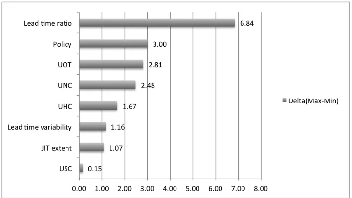
Taguchi’s method (Roy, 1990) is an alternative to factorial design that allows the analysis of many parameters without many experiments. By using Taguchi’s orthogonal arrays, only 18 experiments are necessary in this case. After conducting the experiments, we computed for each factor j the value ∆j, which in the Taguchi’s analysis is used

to make judgements about the importance of the factors. Factors are ranked from the highest ∆j, having the highest contribution toward the cost to the lowest ∆j, having the

lowest contribution toward the cost (Figure 4). The description of the design of experi-ments and the detailed calculation of the Taguchi’s analysis can be found in Appendix B.

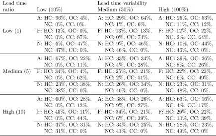
A: HC: 96%, OC: 4%, A: HC: 29%, OC: 64%, A: HC: 25%, OC: 53%, NC: 0%, CC: 0%. NC: 1%, CC: 6%. NC: 11%, CC: 12%. Low (1) F: HC: 13%, OC: 0%, F: HC: 13%, OC: 13%, F: HC: 12%, OC: 22%, NC: 0%, CC: 87%. NC: 0%, CC: 74%. NC: 2%, CC: 64%. N: HC: 6%, OC: 47%, N: HC: 9%, OC: 46%, N: HC: 10%, OC: 44%,

NC: 47%, CC: 0%. NC: 46%, CC: 0%. NC: 46%, CC: 0%. A: HC: 67%, OC: 22%, A: HC: 33%, OC: 34%, A: HC: 39%, OC: 26%,

NC: 0%, CC: 11%. NC: 4%, CC: 28%. NC: 8%, CC: 26%. Medium (5) F: HC: 34%, OC: 4%, F: HC: 25%, OC: 21%, F: HC: 22%, OC: 23%,

NC: 0%, CC: 62%. NC: 2%, CC: 51%. NC: 6%, CC: 49%. N: HC: 23%, OC: 38%, N: HC: 26%, OC: 34%, N: HC: 23%, OC: 31%,

NC: 38%, CC: 0%. NC: 40%, CC: 0%. NC: 48%, CC: 0%. A: HC: 60%, OC: 28%, A: HC: 38%, OC: 26%, A: HC: 63%, OC: 16%,

NC: 0%, CC: 12%. NC: 9%, CC: 27%. NC: 4%, CC: 17%. High (10) F: HC: 45%, OC: 11%, F: HC: 34%, OC: 21%, F: HC: 29%, OC: 22%,

NC: 0%, CC: 44%. NC: 6%, CC: 39%. NC: 10%, CC: 39%. N: HC: 37%, OC: 31%, N: HC: 34%, OC: 25%, N: HC: 28%, OC: 23%, NC: 31%, CC: 0% NC: 41%, CC: 0% NC: 49%, CC: 0%

Table III.: Simulation results: cost breakdown (HC, OC, NC and CC mean holding cost, overtime cost, non-completion cost and changeover cost, respectively).

will be more relevant. Surprisingly lead time variability is found to have little influence on cost. This finding should be understood with care. Because we calculate lead time variability as a percentage of the standard deviation of the mean supply lead time, its effects depend first on the supply lead time as longer supply lead time means higher lead time variability. As a lesson learnt, the company should direct their efforts toward supply lead time reduction because shorter lead time means lower lead time variability.

5. Discussion and conclusions

The analysis performed by this research yields some new observations. Previous studies argued that the benefits of tracking technologies often do not justify their investment expenditures (Sari, 2010). On the contrary, we show that a GPS-based application, com-bined with the ‘Dynamic algorithm’, could be relevant to firms operating in a JIT or perishable supply environment, for which the gains ensuing from the introduction of tracking technologies are relevant. Simulation experiments show that the ‘Dynamic al-gorithm’ outperforms commonly used scheduling policies. Such GPS- and RFID-based real-time tracking technologies were useful in supply chains for generating express or-ders (Gaukleret al., 2008) and for sharing collaborative information (Sari, 2010). This paper shows that final assemblers can use GPS-enabled real-time transport information for production re-scheduling to save important costs.

To our knowledge, this research study is the first to propose dynamic policies con-sidering not only the state of order completion in the production system, but also the progress of raw-material transport directed to the final production plant, under supply and production uncertainties. Previous studies on dynamic policies are based exclusively on the order progress in the production system (Hausman and Scudder, 1982; Wein and Ou, 1991 and Gong et al., 2011). Our study is consistent with this body of literature because they showed, as we did, that dynamic policies based on current system status perform better than static policies. Other studies considering inventory and scheduling problems in the same research tend to focus on demand uncertainty only (Leachman and Gascon, 1988 and Gallego, 1990). Moreover, similar attempts to study dynamic schedul-ing rules tend to focus on assembly processschedul-ing lead time uncertainty but not on supply lead time uncertainty. With a more realistic setting based on an industrial example, this paper provides some new understanding about the use of dynamic scheduling rules for final assemblers facing long and variable supply lead times.

Results from a sensitivity analysis performed with Taguchi’s method show that longer supply lead times could exacerbate the adverse effects of supply uncertainty. This result is consistent with the study of Gaukleret al.(2008), who investigated by simulation the use of dynamic expediting policies when order progress information is available. They found, as we did, that the performance of their dynamic policies deteriorated among long supply lead times. The ‘Dynamic algorithm’ is less effective when lead time variability is medium combined with medium and high ratio between supply and production lead times. In any other case it performs really well (Table II). Based on different settings without using dynamic scheduling rules, Sari (2010) found more benefits when firms in a supply chain collaborate by sharing real-time demand information under long supply lead times. With these results, companies operating under such supply and production uncertainties and JIT supply environment should focus on reducing supply lead time and its variability, and if these measures are impossible, then dynamic scheduling rules like ours can be considered. Based on a cost-breakdown analysis, we also found that the ‘Dynamic algorithm’ works really well when changeovers are expensive and holding costs are low (Table III).

completion of the order in a supply chain. In addition, this paper addresses the problem of modelling supply and production lead time variability. Tang and Grubbstr¨om (2003) and Louly et al. (2008) assume for production lead times discrete distributions and continuous density functions, respectively. Commonly used continuous density functions to model lead times in operations management include the normal distribution, which is unsuitable as it could lead to negative values of lead times, and the Erlang distribution, used by Tang and Grubbstr¨om (2003), which may not be realistic in this setting. This paper applies a continuous lognormal distribution to model supply and production lead time variability, based on verification from the industrial example.

This study provides some foundations for future research. First, a possible extension of this paper could contribute to the more theoretical literature on heuristic scheduling mentioned above considering the uncertainties of the supply and production processes. This contribution could be based on the approximate-stochastic-dynamic programming framework. Second, the application of the ‘Dynamic algorithm’ provides cost reduction benefits but also requires much higher coordination with line supervisors and workers, because of schedule changes in the middle of the work. To investigate what are the precise effects of the adoption of this application on workers behaviour through in-depth case studies would be of interest.

Acknowledgements

The authors would like to thank Mr. Pietro Lucidi, IT project manager, for his kind participation in this research project, Ms. Alice Tasin and Ms. Fen Ren, for helping refining the assumptions of this paper, by working on similar yet different problems, the editor and the anonymous reviewers for their helpful comments and suggestions.

References

Aitchison, J. and Brown, J.A.C., 1957. The lognormal distribution. Cambridge, UK: Cambridge University Press.

Arthur, C., 2011. Thailand’s devastating floods are hitting PC hard drive sup-plies, warn analysts. The Guardian [online], 25 October. Available at: http://www.theguardian.com/technology/2011/oct/25/thailand-floods-hard-drive-shortage [Accessed 18 November 2013].

Bakshi, N., Flynn, S.E. and Gans, N., 2011. Estimating the Operational Impact of Con-tainer Inspections at International Ports. Management Science, 57(1), 1–20.

Ballest´ın, F., P´erez, ´A., Lino, P., Quintanilla, S. and Valls, V., 2013. Static and dynamic policies with RFID for the scheduling of retrieval and storage warehouse operations. Computers and Industrial Engineering, 66(4), 696–709.

Conway, R.W., Maxwell, W.L. and Miller, L., 1967.Theory of scheduling.Reading, MA, USA: Addison-Wesley.

Ding, F–Y. and Sun, H., 2004. Sequence alteration and restoration related to sequenced parts delivery on an automobile mixed model assembly line with multiple depart-ments. International Journal of Production Research, 42(8), 1525–1543.

Fenton, L.F., 1960. The sum of log-normal probability distributions in scatter transmis-sion systems.IRE Transactions on Communication Systems, 8(1), 57–67.

Gallego, G., 1990. Scheduling the production of several items with random demands in a single facility. Management Science, 36(12), 1579–1592.

Gaukler, G.M., ¨Ozer, ¨O. and Hausman, W.H., 2008. Order progress information: im-proved dynamic emergency ordering policies. Production and Operations Manage-ment, 17(6), 599–613.

GIS Park, 2011. Design of Production Scheduling of Commodity Concrete Based on GPS [online]. GIS Park. Available from: http://www.gispark.net/3s-articles/global- position-system/design-of-production-scheduling-of-commodity-concrete-based-on-gps.html [Accessed 21 May 2012].

Ghadge, A., Dani, S. and Kalawsky, R., 2013. Supply chain risk management: present and future scope. The International Journal of Logistics Management, 23(3), 313–339. Gong, J., Prabhu, V.V. and Liu, W., 2011. Simulation-based performance comparison

between assembly lines and assembly cells with real-time distributed arrival time control system. International Journal of Production Research, 49(5), 1241–1253. Hausman, W.H and Scudder, G.D., 1982. Priority scheduling rules for repairable

inven-tory systems. Management Science, 28(11), 1215–1231.

Kim, I. and Springer, M., 2008. Measuring endogenous supply chain volatility: beyond the bullwhip effect.European Journal of Operational Research, 189, 172–193. Leachman, R.C. and Gascon, A., 1988. A heuristic scheduling policy for multi-item,

single-machine production systems with time-varying, stochastic demands. Manage-ment Science, 34(3), 377–390.

Law, A., 2006.Simulation Modeling and Analysis. Maidenhead, UK: McGraw Hill Higher Education.

Louly, M–A., Dolgui, A. and Hnaien, F., 2008a. Supply planning for single-level assem-bly system with stochastic component delivery times and service-level constraint. International Journal of Production Economics, 115, 236–247.

Louly, M–A., Dolgui, A. and Hnaien, F., 2008b. Optimal supply planning in MRP envi-ronments for assembly systems with random component procurement times. Inter-national Journal of Production Research, 46(9), 5441–5467.

Micheli, G.J., Mogre, R. and Perego, A., 2014. How to Choose Mitigation Measures for Supply Chain Risks. International Journal of Production Research, 52(1), 117–129. Olhager, J., 2003. Strategic positioning of the order penetration point. International

Journal of Production Economics, 85(3), 319–329.

Pawar, K. and Rogers, H., 2013. Contextualising the holistic cost of uncertainty in out-sourcing of manufacturing supply chains. Production Planning and Control, 24(7), 607–620.

Rossi, A. and Dini, G., 2000. Dynamic scheduling of FMS using a real-time genetic algorithm.International Journal of Production Research, 38(1), 1–20.

Roy, R.K., 1990. A Primer on the Taguchi method. Dearborn, MI, USA: Society of Manufacturing Engineers.

Sun, L., Heragu, S.S., Chen, L. and Spearman, M.L., 2012. Comparing dynamic risk-based scheduling methods with MRP via simulation. International Journal of Pro-duction Research, 50(4), 921–937.

Tang, O. and Grubbstr¨om, R.W., 2003. The detailed coordination problem in a two-level assembly system with stochastic lead times. International Journal of Production Economics, 81-82, 415–429.

Tomlin, B., 2006. On the value of mitigation and contingency strategies for managing supply chain disruptions risks. Management Science, 52(5), 639–657.

Wang, J., Li, X. and Zhu, X., 2012. Intelligent dynamic control of stochastic economic lot scheduling by agent-based reinforcement learning. International Journal of Pro-duction Research, 50(16), 4381–4395.

Wein, L.M. and Ou, J., 1991. The impact of processing time knowledge on dynamic job-shop scheduling.Management Science, 37(8), 1002–1014.

Zhang, L., Gao, L. and Li, X., 2013. A hybrid genetic algorithm and tabu search for a multi-objective dynamic job shop scheduling problem. International Journal of Production Research, 51(12), 3516–3531.

Zsidisin, G.A., 2003. A grounded definition of supply risk. Journal of Purchasing & Supply Management, 9(5–6), 217–224.

Appendix A. Proof of Proposition 3.1

LetX1. . . XKbeKindependent and identical lognormal variables representing the travel

time to cover each road segment of a particular route. The lognormal variables are char-acterised by a mean µXi and a standard deviation σXi for each i = 1. . . K. Each Xi can be written as exp(Yi), with each Yi as a normal variable with mean µYi and a stan-dard deviationσYi. Therefore, the lead time for a particular route from a supplier to the

company can be represented by the compound distribution of K lognormal variables. Unfortunately, no exact result is known for this resulting distribution. Thus we estimate the lead time distribution for a route by using the Fenton-Wilkinson approximation (Fen-ton, 1960, p. 60) as follows. The Fenton-Wilkinson method approximates the sum of the K independent lognormal variables with a lognormal variable X, with meanµX and a

standard deviation σX, obtained by matching the first and second central moments of

X with that of the sum of Xi fori= 1. . . K, as given by:

µX =K·µXi, (A1a)

σ_X2 =K·σ_X2i. (A1b)

The lognormal variableX can then be written as exp(Y), withY as a normal variable with mean µY and a standard deviation σY. Knowing the parameters µX and σX2 ,µY

µY = ln





µ2_X

q

µ2

X+σX2



, (A2a)

σ_Y2 = ln

1 + σ 2 X µ2 X . (A2b)

Because Y is normally distributed, it is easy to numerically determine its cumulative distribution function FY and its inverse F_Y−1 when µY and σ_Y2 are given. We assign

a raw material in stock before the day of production if the delay associated with the customer service levelF−1

X (CSL, µX, σ

2

X) is more than the thresholdt. The delay can be

expressed asF−1

X (CSL, µX, σX2)−µX. Finally, because of the relationship between the

normal distribution and the lognormal distribution the condition for assigning a stock unit can be written as follows:

F−1

X (CSL, µX, σ

2

X)−µX = exp(F_Y−1(CSL, µy, σy)−µx≥t (A3)

Appendix B. Details of Taguchi’s analysis

In our setting we use Taguchi’s orthogonal array L18 that involves 18 experiments. The array has been defined by testing combinations of parameters instead of single parameters and derives from a statistical technique, which selects the experiments denser in information. However, Taguchi’s array L18 allows us to test seven parameters with three levels and one parameter with two levels. Therefore, it is necessary to eliminate one level from our analysis. We decided to remove the ‘No changes’ scheduling policy from the analysis because it performed relevantly worse compared with the ‘Dynamic algorithm’ and FIFO policies as could be seen from the results of Table II. The 18 experiments derived from Taguchi’s technique are shown in Table B1.

Taguchi’s method analyses the experiments based on the calculation of the signal-to-noise ratio for each experiment. We respectively denote the mean and the variance of the value of interest across the replications performed for the experimentias ¯yi and s2_i.

Then the signal-to-noise ratioSNi for the experimentican be computed as follows:

SNi= 10 log

¯ y_i2 s2

i

. (B1)

As the assessment of each experiment i is based on the measure SNi, which directly

considers the variance s2_i of the experiment, it is paramount that the number of runs is the same for each experiment. We set the number of runs to 5,000 because this number, as could be seen in the simulation results of Table II, should, usually, guarantee a confidence interval of 5% with an indifference zone of 50. The values ofSNifor each experimentiare

shown in Table B2. After calculatingSNi for each experimentiit is possible to compute

the average SNj,k for each factor j and each level k. This is obtained by averaging all

the experiments based on the factor j and the level k. Finally, for each factor j the value ∆j is computed as the difference between the highest value and the lowest value of

T8 A 10 15 1 1,000 250 15 100 14.44

T9 F 10 0 0.1 1,250 500 5 200 9.10

T10 F 1 30 1 1,250 500 10 100 4.21

T11 F 1 15 0.1 750 750 15 200 9.79

T12 F 1 0 0.5 1,000 250 5 300 7.76

T13 F 5 30 0.5 1,250 250 15 200 11.70

T14 F 5 15 1 750 500 5 300 12.85

T15 F 5 0 0.1 1,000 750 10 100 10.62

T16 F 10 30 1 1,000 750 5 200 11.44

T17 F 10 15 0.1 1,250 250 10 300 13.45

T18 F 10 0 0.5 750 500 15 100 13.96

Table B1.: Taguchi’s method experiments

Factor SN1,k SN2,k SN3,k ∆j Rank

Policy A: 7.64 F: 10.64 – 3.00 2 Ratio 1: 5.17 5: 10.25 10: 12.01 6.84 1 JIT 30: 8.67 15: 9.74 0: 9.01 1.07 7 Variability 0.1: 9.66 0.5: 8.50 1: 9.26 1.16 6 UOT 750: 10.53 1,000: 9.18 1,250: 7.72 2.81 3 UNC 250: 10.71 500: 8.49 750: 8.23 2.48 4 UHC 5: 8.88 10: 8.44 15: 10.11 1.67 5 USC 100: 9.23 200: 9.12 300: 9.08 0.15 8

Table B2.: Taguchi’s method results

contribution toward the cost to the lowest ∆j, having the lowest contribution toward the