Occupation time distributions for the telegraph process

This is a repository copy of Occupation time distributions for the telegraph process. White Rose Research Online URL for this paper:

http://eprints.whiterose.ac.uk/74927/

Article:

Bogachev, L and Ratanov, N (2011) Occupation time distributions for the telegraph process. Stochastic Processes and their Applications, 121 (8). 1816 - 1844 (29). ISSN 0304-4149

https://doi.org/10.1016/j.spa.2011.03.016

Reuse See Attached

Takedown

If you consider content in White Rose Research Online to be in breach of UK law, please notify us by

Occupation time distributions for the telegraph process

Leonid Bogacheva,∗_{, Nikita Ratanov}b

a

Department of Statistics, School of Mathematics, University of Leeds, Leeds LS2 9JT, UK b

Facultad de Econom´ıa, Universidad del Rosario, Cl. 14, No. 4-69, Bogot´a, Colombia

Abstract

For the one-dimensional telegraph process, we obtain explicitly the distribution of the occupation time of the positive half-line. The long-term limiting distribution is then derived when the initial location of the process is in the range of sub-normal or normal deviations from the origin; in the former case, the limit is given by the arcsine law. These limit theorems are also extended to the case of more general occupation-type functionals.

Keywords: Telegraph process; Telegraph equation; Feynman–Kac formula; Weak convergence; Arcsine law; Laplace transform

2000 MSC:primary 60J27; secondary 60J65, 60F05, 60K99

1. Introduction

LetB = (Bt, t≥0) be a standard Brownian motion onR starting from the origin

(B0 = 0), and consider the occupation time functional

hT :=

1 T

Z T

0

H(Bt) dt, T >0, (1.1)

whereH(x) is the Heaviside unit step function (i.e., H(x) = 0 forx_≤0 andH(x) = 1 forx >0). That is to say, hT ∈[0,1] is the proportion of time spent by the Brownian

motion (Bt, 0≤t≤T) on the positive half-line. It is well known that the probability

distribution of the random variable hT does not depend on T (which is evident from

the scaling property of the Brownian motion and the fact thatH(αx)≡H(x) for any α >0) and is given by the classic arcsine law,

P{h_{T ≤}y}= 2

π arcsin

√

y, 0≤y ≤1, (1.2)

with the probability density

pas(y) :=

1

πpy(1−y), 0< y < 1. (1.3)

∗_{Corresponding author.}

Email addresses: [email protected](Leonid Bogachev),[email protected]

The beautiful formula (1.2) dates back about 70 years to P. L´evy [Le40, Th´eor`eme 3, pp. 301–302], who has also proved that the arcsine law (1.2) is the limit distribution for the relative frequency of positive sums among consecutive partial sums of independent symmetric Bernoulli (0–1) random variables [Le40, Corollaire 2, p. 303]. Using the invariance principle, the latter result was extended by P. Erd˝os and M. Kac [EKa47] to the case of sums of arbitrary i.i.d. random variables with zero mean and unit variance (cf. [St93, Theorem 4.3.19, p. 236]). More recently, R. Khasminskii [Kh99] obtained the limit distribution, as T _{→ ∞}, of more general functionals of the form

hT(x;f) :=

1 T

Z T

0

f(x+Xt) dt,

where Xt (X0 = 0) is a diffusion process on R with generator L = a(x) d2/dx2, and

f : _{R → R} is a probing function from a suitable class. In particular, the results of [Kh99] imply that if limx→±∞a(x) =a0 >0 and f is a bounded piecewise continuous

function such that

lim

x→±∞

1 x

Z x

0

f(u) du=f_±, f+ 6=f−, (1.4)

then the distribution of the random variable (hT(x;f)−f−)/(f+−f−) converges weakly,

asT → ∞, to the arcsine law (1.2).

In the present paper, we obtain similar results for the so-called telegraph process

defined by

Xt :=V0

Z t

0

(₋1)Nu

du, t_≥0, (1.5)

where (Nt, t≥0) is a homogeneous Poisson process (with rate λ >0), V0 is a random

variable with equiprobable values _±c independent of the process Nt, and c > 0 is a

parameter (see [Go51, Ka74, Pi91]). That is, Xt is the position at time t ≥ 0 of a

particle starting at t = 0 from the origin and moving on the line with alternating velocities _±c, reversing the direction of motion at each jump instant of the Poisson process Nt; the initial (random) direction is decided by the sign of V0. Note that

the process Xt itself is non-Markovian, however if Vt = dXt/dt = (−1)NtV0 is the

corresponding velocity process, then the joint process (Xt, Vt) is Markov on the state

spaceR× {−c,+c_}(see [EtK86, _§12.1, p. 469]). We shall also consider the conditional telegraph processes obtained fromXt by conditioning on V0,

X_t± :=±c Z t

0

(−1)Nu

du, t≥0, (1.6)

where the choice of the + or − sign determines the initial direction of motion.

Remark 1.1. Here and throughout the paper, we adopt a notational convention that any formula involving the _±and _∓ signs combines the two cases corresponding to the choice of either the upper or lower sign, respectively.

The model of non-interacting particles moving in one dimension with alternating velocities (updated at random on a discrete time grid) was first introduced in 1922 by G. I. Taylor [Ta22] in an attempt to describe turbulent diffusion; later on (around 1938–1939) it was studied at length by S. Goldstein [Go51] in connection with a certain hyperbolic partial differential equation (called thetelegraph, ordamped wave equation, see (1.7) below) describing the spatio-temporal dynamics of the potential in a trans-mitting cable (without leakage) [We55]. In his 1956 lecture notes, M. Kac (see [Ka74]) considered a continuous-time version of the telegraph model. Since then, the tele-graph process and its many generalizations have been studied in great detail (see, e.g., [Or90, Pi91, FK94, Or95, Ra99, We02]), with numerous applications in physics [We02], biology [Ha99, HH05], ecology [OL01] and, more recently, financial market modelling [Ra07, RM08] (see also further bibliography in these papers).

An efficient conventional approach to the analytical study of the telegraph process, analogous to that for diffusion processes, is based on pursuing a fundamental link relating various expected values of the process with initial value and/or boundary value problems for certain partial differential equations (see, e.g., [Go51, Or90, Or95, Ra97, Ra99, Ra06]). In particular, Kac [Ka74] has shown that, for any bounded continuously differentiable function g0 :R→R, the functions

v±(x, t) :=E£g0(x+Xt±)

¤

, x_∈R, t_≥0,

satisfy the set of partial differential equations

∂v±(x, t)

∂t ∓c

∂v±(x, t)

∂x =∓λ

¡

v+(x, t)−v−(x, t)¢

, t >0,

with the initial conditions

v±_{(x,0) =g}

0(x), x∈R.

These equations can be easily combined (see details in [Ka74] or [EtK86,_§12.1, p. 470]) to show that the function

v(x, t) :=E[g0(x+Xt)] =

1 2v

−_{(x, t) +} 1

2v

+_{(x, t)}

satisfies the telegraph (or telegrapher’s) equation (see, e.g., [We55, _§15])

∂2_v

∂t2 + 2λ

∂v ∂t =c

2∂2v

∂x2 (1.7)

with the initial conditions

v(x,0) = g0(x),

∂v

∂t(x,0) = 0. (1.8)

The (unique) solution of the Cauchy problem (1.7)–(1.8) can be written explicitly (see, e.g., [We55,_§§46, 74] or [Pi91, _§0.4]) as

v(x, t) = 1 2e

−λt¡

g0(x+ct) +g0(x−ct)

¢

+ 1 2e

−λtZ t

−t

g0(x+cu)

µ λI0

¡

λ√t2_−u2¢

+√ λt

t2_−u2 I1

¡

λ√t2_−u2¢ ¶

du,

(1.9) where

I0(z) :=

∞

X

n=0

(z/2)2n

(n!)2 and I1(z) :=I

′

0(z) =

z 2

∞

X

n=0

(z/2)2n

n! (n+ 1)! (z ∈R)

are the modified Bessel functions of the first kind (of orders 0 and 1), respectively) [AS72, 9.6.12, p. 375; 9.6.27, p. 376].

It is well known that, under a suitable scaling, the telegraph process satisfies a functional central limit theorem.

Theorem 1.1. Assume that λ, c → +∞ in such a way that c2_{/λ → 1. Then the}

distribution of the telegraph processes (Xt±, t ≥ 0) converges weakly in C[0,∞) to the

distribution of a standard Brownian motion (Bt, t ≥ 0). The same is true for the

unconditional telegraph process (Xt, t ≥0).

As was observed by Kac [Ka74, p. 501], this result formally follows from the tele-graph equation (1.7), which in the limit λ, c _→ +_∞, c2_{/λ → 1 yields the diffusion}

(heat) equation

∂v ∂t =

1 2

∂2_v

∂x2,

associated with the standard Brownian motion Bt. A rigorous proof of Theorem 1.1,

along with some extensions, can be found in [EtK86,_§12.1, p. 471] and [Ra99, Theorem 5.1] (see also [Or90, §4] for a density version).

Our main goal in the present paper is to analyze the distribution of the occupation time of the telegraph process Xt and, in particular, to obtain a limit distribution, as

T → ∞, of the occupation-type functionals of the formηT(x;f) :=T−1

RT

0 f(x+Xt) dt

for a suitable class of probing functions f. In particular, we prove that the limit distribution is given by L´evy’s arcsine law providing that the starting point x is in the range of subnormal deviation from the origin (i.e., x = o(√T )). For technical simplicity, we impose a stronger condition on the asymptotics of f at ±∞, assuming that the corresponding limitsf_± exist.

2. Statement of the main results

ForT > 0, x_∈R, consider the following occupation time random variables

ηT(x) :=

1 T

Z T

0

H(x+Xt) dt, η±T(x) :=

1 T

Z T

0

H(x+X_t±) dt, (2.1)

where H(x) = 1(0,∞)(x) is the Heaviside step function and Xt, Xt± are the telegraph

processes introduced above (see (1.5), (1.6)). Note that the total time spent by the processes (x+X_t±, 0_≤t _≤ T) at the origin almost surely (a.s.) equals zero, since by Fubini’s theorem we have

E

Z T

0

1{0}(x+Xt±) dt=

Z T

0 P{

X_t± =₋x_}dt = 0. (2.2)

Hence, the complementary quantity 1−η±_T(x) a.s. equals the proportion of time spent by the processes (x+Xt±, 0≤t≤T) on the negative side of the axis,

1−η_T±(x) = 1 T

Z T

0

1(−∞,0)(x+Xt±) dt (a.s.),

and by symmetry (with respect to simultaneous transformationsx_{7→ −}x, _{± 7→ ∓}) it follows that

η±_T(x)= 1d ₋η_T∓(₋x), x_∈R. (2.3) Let us consider the functionϕT(t) (t ≥0) defined by

ϕT(t) :=

1 4πλT

Z t

0

1₋e−2λT u

u3/2√_t−udu (t >0), ϕT(0) :=

1

2. (2.4)

After the substitutionu=ty, we have in the limit as t_↓0,

ϕT(t) =

1 4πλT t

Z 1

0

1₋e−2λT ty

y3/2√_1−ydy→

1 2π

Z 1

0

1 p

y(1−y)dy= 1

2 (2.5)

(see (1.3)), and soϕT(·) is continuous at zero (and hence everywhere on [0,∞)). Note

the following useful scaling relation, which easily follows from the representation of ϕ given by (2.5):

ϕαT(t) = ϕT(αt), t ≥0, α >0. (2.6)

Let us also set

ψT(y) := 2λT ϕT(y)ϕT(1−y), 0≤y≤1. (2.7)

We are now ready to state our first result.

Theorem 2.1. The random variables η±_T(0) defined in (2.1) have the distribution

P©η±_T(0)∈dyª

= 2ϕT(1)δx±(dy) +ψ_T(y) dy, 0≤y≤1, (2.8)

where δx is the Dirac measure (of unit mass) at point x, with x−= 0, x+= 1.

Fur-thermore, the distribution of ηT(0) (see (2.1)) is given by the formula

P©

In other words, the distribution of η−_T(0), η_T+(0) has a discrete part with atom of mass 2ϕT(1) at point 0 or 1, respectively, and an absolutely continuous part with the

densityψT defined by (2.7). Similarly, the distribution of ηT(0) has atoms at points 0

and 1, both of massϕT(1), and an absolutely continuous part with the density ψT as

above.

Remark 2.1. The _±-duality in (2.8) becomes clear from relation (2.3) (withx= 0) and the symmetry propertyψT(y)≡ψT(1−y) (see (2.7)).

Remark 2.2. Using an integral formula (see [AS72, 9.6.16, p. 376]) for the modified Bessel function I0, it is easy to check that the function ϕT defined by (2.4) admits

another representation,

ϕT(t) =

1 2λT t

Z λT t

0

e−y_I

0(y) dy, t >0,

which is further evaluated (see [AS72, 11.3.12, p. 483]) to yieldϕT(t) = 1₂e−λT t

¡

I0(λT t)

+I1(λT t)

¢

. Thus, the distribution of η_T±(0) and ηT(0) can be expressed through the

modified Bessel functionsI0 andI1, as well as the distribution of the telegraph process

(cf. (1.9)).

In the next theorem, we give explicit integral formulas for the distribution ofη_T±(x) in the casex₆= 0. For simplicity, we only present the answer for x <0, the casex >0 readily following in view of the duality relation (2.3).

Theorem 2.2. Assume that x < 0 and set T0 := |x|/c. Then, for any T > 0, the

random variables η_T±(x) defined in (2.1) have the following distribution: (a) if T ≤T0 then P{ηT±(x) = 0}= 1;

(b) if T > T0 then, for 0≤y≤1−T0/T,

P{η_T±(x)∈dy}= µZ _∞

T

Q±_−x(u) du ¶

δ0(dy) +µ±T(dy) +Ψx±(y, T) dy, (2.10)

where µ−_T(dy) := 0 and

µ+_T(dy) := 2 e−λT0

ϕT(1−T0/T)δ1−T0/T(dy) + e− λT0

ψT−T0

µ y 1−T0/T

¶ dy 1−T0/T

,

(2.11)

Ψ_x±(y, T) := 2T Q±_−x((1₋y)T)ϕT(y) +

Z (1−y)T

T0

Q±_−x(u)ψT−u

µ y 1−u/T

¶ du 1−u/T ,

(2.12)

withϕT andψT given by (2.4) and (2.7),respectively,and the functions Q±₋x(u) (−x >

0)defined for all u_∈[T0,∞) by

Q+_−x(u) := λT0e−

λu

p

u2_−T2 0

I1

¡

λpu2_−T2 0

¢

, (2.13)

Q−_−x(u) :=λe−λuI0¡λ

p

u2_−T2 0

¢

−λ(u−T0) e−

λu

p

u2_−T2 0

I1¡λ

p

u2_−T2 0

¢

For the next theorem, we need a few notations. For a >0, consider the function

qa(t) :=

a

√

2πt3 exp

µ

−a

2

2t ¶

, t >0, (2.15)

with Laplace transform (see [AS72, 29.3.82, p. 1026])

Z ∞

0

e−stqa(t) dt= e−a

√

2s_{, s}

≥0. (2.16)

Let Ya (a ≥ 0) be a family of random variables with values in [0,1], such that Y0

has the arcsine distribution (1.2), with the density pas (see (1.3)), while for a > 0 the

distribution ofYa is given by

P{Ya ∈dy}=maδ0(dy) +fa(y) dy, (2.17)

where

ma:=

Z ∞

1

qa(u) du=

2

√

2π Z a

0

e−y2/2dy, (2.18)

fa(y) :=

Z 1−y

0

qa(u)

1−upas µ

y 1−u

¶

du= pa 2π3_y

Z 1−y

0

e−a2_/(2u)

u3/2√_1−y−udu . (2.19)

Remark 2.3. It is easy to verify, either from (2.15) or using the Laplace transform (2.16), thatqa

w∗

→δ0 asa→0+, whereδ0(·) is the Dirac delta function and

w∗

→ denotes weak-∗ _{convergence of generalized functions; hence m}

a → 0 (which can also be seen

directly from the right-hand side of (2.18)) and fa w∗

→pas (see the first part of formula

(2.19)). That is, Ya d

→ Y0 as a → 0+, and so the distribution of Ya is continuous in

parametera _∈[0,_∞).

Theorem 2.3. Suppose that the initial position X₀± = x, as well as the parameters c

and λ, may depend on T in such a way that λT → ∞ and (c2_T/λ)−1/2_{x→ a ∈ R as}

T _{→ ∞}. Then, as T _{→ ∞},

ηT(x), η±T(x) d

−→

½

Y₋a, a≤0,

1₋Ya, a≥0.

(2.20)

In particular, for a= 0 the limit is given by the arcsine distribution (1.2).

To order to generalize these results in the spirit of [Kh99], let f : R → R be a bounded, piecewise continuous function (i.e., continuous on R outside a finite set Df,

where it has finite left and right limits), such that, for some finite constants f+ 6=f−,

lim

x→−∞f(x) =f−, x→lim+∞f(x) = f+. (2.21)

Consider the random variables

η_T±(x;f) := 1 (f+−f−)T

Z T

0

¡

f(x+X_t±)−f₋¢

Clearly, by a linear transformation of the function,

f(x)7→f˜(x) := f(x)−f− f+−f−

, x∈R, (2.23)

we may and will assume without loss of generality thatf₋= 0, f+= 1, so that (2.22)

is reduced to

η±_T(x;f) := 1 T

Z T

0

f(x+X_t±) dt. (2.24)

Theorem 2.4. Let the function f satisfy the above conditions including assumption

(2.21) with f₋ = 0, f+ = 1. Suppose that the hypotheses of Theorem 2.3 are satisfied,

and assume in addition that c2_{T/λ→ ∞asT → ∞. Then the distribution of η}±

T(x;f)

converges weakly, as T _{→ ∞}, to the law determined by the right-hand side of (2.20).

Remark 2.4. We conjecture that Theorem2.4holds under a weaker assumption (1.4) of Ces`aro-type averaging of the probing functionf at _±∞, replacing the limit condition (2.21). It seems plausible that the analytic techniques developed in the paper (espe-cially in Section 7) may be suitably adjusted to this effect, and we will address this problem elsewhere. Some numerical evidence in favour of our conjecture is presented below in Section8.

3. The Feynman–Kac formula and applications

Let us recall the Feynman–Kac formula for the telegraph processes.

Theorem 3.1. Let (X_t±, t_≥ 0) be the telegraph processes (1.6). Suppose that g0 and

g are bounded functions on _R such that g0 ∈C1(R) andg is piecewise continuous, i.e.,

g ∈C(R\Dg), where Dg is a finite set,and moreover, g has finite left and right limits

at the points of Dg. Then the functions

v±(x, t) := E

·

g0(x+Xt±) exp

½Z t

0

g(x+X_u±) du ¾¸

, x∈R, t≥0, (3.1)

for all (x, t) ∈ R× R+ such that x± ct /∈ Dg satisfy the set of partial differential

equations

∂v±_{(x, t)}

∂t ∓c

∂v±_{(x, t)}

∂x =∓λ

¡

v+(x, t)₋v−(x, t)¢

+g(x)v±(x, t),

with the initial conditions

v±(x,0) =g0(x), x∈R.

Letη_T±(x) be defined by (2.1). For β _∈R, set

v_T±(ξ, t) :=E£e−βt ηT t±(cT ξ)¤, ξ ∈R, t≥0, (3.2)

or more explicitly (cf. (3.1))

v±

T(ξ, t) = E

· exp

½

−β T

Z T t

0

H(cT ξ+X±

u) du

¾¸

, ξ_∈R, t_≥0. (3.3)

SinceH(_·) is a bounded function, the expectation in (3.3) is finite for allβ _∈R. Let us record some simple properties of the function v_T±.

Lemma 3.2. For eachβ ∈R and any T >0, the functions v_T±(ξ, t) are continuous in each variable on _R×R+ and

lim

ξ→−∞v

±

T(ξ, t) = 1, lim ξ→+∞v

±

T(ξ, t) = e−βt. (3.4)

Proof. Continuity int_∈R+ is obvious. As mentioned above (see (2.2)), for anyξ0 ∈R

we have a.s. that cT ξ0 +Xu± 6= 0 for all u ∈ [0, T t] except on a (random) set of

Lebesgue measure zero. Since the function H is continuous outside zero, this implies that, for suchu,H(cT ξ+X±

u)

a.s.

−→H(cT ξ0+Xu±) asξ→ξ0 and hence, by Lebesgue’s

dominated convergence theorem, RT t

0 H(cT ξ +Xu±) du

a.s.

−→ RT t

0 H(cT ξ0 +Xu±) du as

ξ → ξ0. The continuity of vT±(·, t) at point ξ0 now follows by Lebesgue’s dominated

convergence theorem applied to the expectation (3.3), since everything is bounded (for a fixed t).

To prove (3.4), note that, for T > 0 and each u ≥ 0, we have cT ξ +X±

u

a.s.

−→ ±∞ as ξ _{→ ±∞}. Since H is bounded on _R, the claim now follows by dominated convergence.

From the definition (3.3), it is clear that ifβ _≥0 then, for eachξ_∈R, the functions v_T±(ξ,·) are bounded on [0,∞), so we can define the Laplace transform

w±_T(ξ, s) := Z ∞

0

e−stv_T±(ξ, t) dt (s >0). (3.5)

Lemma 3.3. Set s˜:=s+β. For any fixed s >0,the functionsw±_T =w_T±(ξ, s)defined by (3.5) are continuous in ξ _∈R and satisfy the following set of differential equations

∂ w±

T

∂ξ =λT ¡

w_T+−w−_T¢

±¡

s+H(cT ξ)¢

w_T±∓1, ξ6= 0. (3.6)

Moreover,

lim

ξ→−∞w

±

T(ξ, s) =s−1, lim

ξ→+∞w

±

Proof. The continuity of the functions w_T±(ξ, s) in ξ follows from the definition (3.5) and the first part of Lemma 3.2. Further, applying Theorem 3.1 (with g0(x)≡ 1 and

g(x) = −β T−1_{H(x)), we see that the functions v}±

T = v±T(ξ, t) defined by (3.2) satisfy

the initial value problem

∓∂vT±

∂t + ∂v_T±

∂ξ =λT ¡

v+_T −v_T−¢

±βH(cT ξ)v±_T, t >0, ξ±t 6= 0, (3.8)

v_T±(ξ,0) = 1, ξ∈R. (3.9)

Integrating by parts and using the initial condition (3.9), we have

Z ∞

0

e−st ∂ v

±

T(ξ, t)

∂t dt=−v

±

T(ξ,0) +s

Z ∞

0

e−stv_T±(ξ, t) dt =−1 +sw±_T(ξ, s). (3.10)

Applying the Laplace transform (with respect to t) to equation (3.8) and taking into account (3.10), we immediately obtain the differential equation (3.6). Finally, the boundary conditions (3.7) readily follow from (3.4) by Lebesgue’s dominated conver-gence theorem applied to (3.5).

Let us also make similar preparations for the random variables η±

T(x;f) defined in

(2.22). As explained in Section2 (see (2.23)), without loss of generality this definition can be simplified to the form (2.24). Consider the functions (cf. (3.2))

v±_T(ξ, t;f) :=E£exp¡

−βtη±_{T t}(cT ξ;f)¢¤

, ξ_∈R, t_≥0,

and the corresponding Laplace transform

w_T±(ξ, s;f) := Z ∞

0

e−stv_T±(ξ, t;f) dt, s >0. (3.11)

Then, again applying Theorem3.1 (withg0(x)≡1 and g(x) =−β T−1f(x)), similarly

to Lemmas 3.2 and 3.3 one can show that w_T± = w_T±(ξ, s;f), for each s > 0, is a continuous bounded function of ξ _∈R, satisfying the differential equation (cf. (3.6))

∂ w±_T ∂ξ =λT

¡

w_T+−w−_T¢

±¡

s+βf(cT ξ)¢

w±_T ∓1, ξ∈R\Df, (3.12)

with the same boundary conditions at_±∞ as (3.7),

lim

ξ→−∞w

±

T(ξ, s;f) = s−

1_{, lim}

ξ→∞w

±

T(ξ, s;f) = ˜s−

1_{. (3.13)}

4. Proof of Theorem 2.1

In what follows, the prime ′ denotes the transposition of vectors. Introducing the vector notations

we can write down equations (3.6) and (3.7) in the matrix form,

∂wT(ξ, s)

∂ξ =AT(ξ, s)wT(ξ, s)−˜1 (ξ6= 0), (4.1) lim

ξ→−∞wT(ξ, s) =s

−1_{1, lim}

ξ→+∞wT(ξ, s) = ˜s

−1_{1, (4.2)}

where ˜s=s+β (see Lemma 3.3) and

AT(ξ, s) :=λT J1+

¡

s+βH(cT ξ)¢ J2

= (

λT J1+sJ2 =:AT ≡AT(s), ξ <0,

λT J1+ ˜sJ2 =: ˜AT ≡AT(˜s), ξ >0,

(4.3)

J1 :=

Ã

1 ₋1 1 ₋1

!

, J2 :=

Ã

1 0

0 ₋1 !

. (4.4)

Note that

J11=0, J1˜1= 2·1, J21= ˜1, J2˜1=1, (4.5)

where0:= (0,0)′_{. Hence (see (4.3))}

AT(s)1=s1˜, AT(s) ˜1= (s+ 2λT)1. (4.6)

Let us set

κ≡κ(s) := ps(s+ 2λT), κ˜:=κ(˜s) =ps˜(˜s+ 2λT). (4.7)

Using formulas (4.6) and (4.7), it is easy to check that the matrix AT(s) has the

eigenvalues±κ(s) with the corresponding eigenvectors

a_±≡a_±(s) := ±κ1+s1˜, ATa± =±κa±. (4.8)

In particular, relations (4.8) imply that the exponential of AT(s) can be represented

as follows:

eATξ

= 1 2 e

κξ¡

I+κ−1AT

¢ +1

2e−

κξ¡

I ₋κ−1AT

¢

, (4.9)

whereI is the identity matrix.

Recall that we are looking for a solution to the boundary value problem (4.1)–(4.2) continuous at the origin. The following lemma gives an explicit form of such a solution.

Lemma 4.1. For each s > 0, the differential equation (4.1) subject to the boundary conditions (4.2) has the unique continuous solution given by

w_T(ξ, s) =    

  

−eκξ βs−

1

s˜κ+ ˜sκ(κ1+s1˜) +s

−1_{1, ξ}

≤0,

e−˜κξ βs˜−

1

s˜κ+ ˜sκ(˜κ1−s˜1˜) + ˜s

−1_{1, ξ}

≥0.

(4.10)

In particular,

w_T(0, s) = (˜κ+κ)1+ (s−s)˜˜ 1

Proof. Observe that the step function w∗

T(ξ, s) :=

¡

s+βH(cT ξ)¢−1

1 is a particular solution of the equation (4.1) for eachs >0 and allξ₆= 0. Indeed, the functionw∗_T(_·, s) is piecewise constant outside zero, hence (∂/∂ξ)w∗_T(ξ, s) = 0 (ξ₆= 0), whereas, due to (4.3) and (4.5),

AT(ξ, s)w∗T(ξ, s) =λT

¡

s+βH(cT ξ)¢−1

J11+J21≡1˜.

Therefore, a general solution of the linear differential equation (4.1) can be repre-sented in the form (see (4.3))

w_T(ξ, s) = (

eATξ_c(s) +s−1₁, ξ <0,

eA˜Tξ_c˜(s) + ˜s−1₁, ξ >0, (4.12)

with arbitrary vectors c(s), ˜c(s) (which may also depend on T). Let us now find suitablec(s) and ˜c(s) so that the solutionwT(·, s) would satisfy the required boundary

conditions at infinity and the continuity condition at zero. From the representation (4.12) it is clear that conditions (4.2) are satisfied if and only if

lim

ξ→−∞e

ATξ

c(s) =0, lim

ξ→+∞e

˜

ATξ

˜

c(s) =0. (4.13)

Recalling that ˜AT(s) =AT(˜s) and using the exponential formula (4.9), it is easy to see

that conditions (4.13) are reduced to the equations

(I₋κ−1AT)c(s) =0, (I+ ˜κ−1A˜T) ˜c(s) =0,

which implies thatc(s) and ˜c(s) are eigenvectors of the matrices AT and ˜AT,

respec-tively, with the corresponding eigenvaluesκand₋κ. On account of formulas (4.8), this˜ immediately gives c(s) = C(s)a+, ˜c(s) = ˜C(s) ˜a−, with some real-valued functions

C(s), ˜C(s). Therefore, after the substitution of expressions (4.8), formula (4.12) takes the form

wT(ξ, s) =

(

eκξ_{C(s)(κ1+s˜1) +s}−1_{1, ξ <0,}

−e−˜κξ_C(s)(˜˜ _{κ1−s˜˜1) + ˜s}−1_{1, ξ >0.} (4.14)

Furthermore, taking into account the continuity of w_T(_·, s) at zero, from (4.14) we have

C(s) (κ1+s˜1) +s−11= ˜C(s) (−κ˜1+ ˜s1˜) + ˜s−11,

whence, by equating the coefficients of 1 and ˜1 on the left- and right-hand sides, we obtain

(

C(s)κ+s−1 =−C(s) ˜˜ κ+ ˜s−1, C(s)s= ˜C(s) ˜s .

Solving this system of equations we find

C(s) = −βs−

1

s˜κ+ ˜sκ, C(s) =˜

−βs˜−1

s˜κ+ ˜sκ,

Lemma 4.2. The components w±_T(0, s) (see (4.11)) are explicitly given by the expres-sions

w+_T(0, s) = 2 ˜ κ+ ˜s +

2λT

(κ+s)(˜κ+ ˜s), (4.15)

w−_T(0, s) = 2 κ+s +

2λT

(κ+s)(˜κ+ ˜s). (4.16)

Proof. From the vector expression (4.11) we have

w±

T(0, s) =

˜

κ_∓s˜+κ_±s

s˜κ+ ˜sκ . (4.17)

Note that, according to (4.7),

κ2 ₋s2 = 2λT s, κ˜2₋˜s2 = 2λTs,˜ (4.18)

hence the expression (4.17) may be rewritten as

w±_T(0, s) = 1 s˜κ+ ˜sκ

µ

κ2_−s2

κ∓s + ˜ κ2_−˜s2

˜ κ±˜s

¶

= 2λT

s˜κ+ ˜sκ µ

s κ∓s +

˜ s ˜ κ±s˜

¶

= 2λT

(κ∓s)(˜κ±s)˜ , (4.19)

which is equivalent to (4.15), (4.16); for instance, for w+_T(0, s) (corresponding to the choice of the upper sign in_±and_∓), from formula (4.19) we obtain, again using (4.18),

w_T+(0, s) = 2λT

(κ₋s)(˜κ+ ˜s) =

2λT(κ+s) (κ2_−s2_{)(˜κ+ ˜s)} =

κ+s s(˜κ+ ˜s)

= 2

˜ κ+ ˜s +

κ₋s s(˜κ+ ˜s) =

2 ˜

κ+ ˜s +

2λT (κ+s)(˜κ+ ˜s),

in agreement with (4.15). Thus, Lemma 4.2 is proved.

Lemma 4.3. Let the function ϕT(t) be defined by (2.4). Then, for each s >0,

Z ∞

0

e−stϕT(t) dt =

1 κ+s,

Z ∞

0

e−ste−βtϕT(t) dt=

1 ˜

κ+ ˜s, (4.20)

and

Z ∞

0

e−st µZ t

0

e−βyϕT(y)ϕT(t−y) dy

¶

dt= 1

(κ+s)(˜κ+ ˜s), (4.21)

where s˜=s+β and κ=κ(s), ˜κ=κ(˜s) are defined in (4.7).

Proof. Inserting (2.4) and changing the order of integration, we obtain

Z ∞

0

e−stϕT(t) dt=

1 4πλT

Z ∞

0

1−e−2λT u

u3/2

µZ _∞

u

e−st

√

t₋udt ¶

du

= Γ(

1 2)

4πλT√s Z ∞

0

e−su¡

1₋e−2λT u¢

Integration by parts viau−3/2_{du=−2 d(u}−1/2_{) yields the right-hand side of (4.22) in}

the form

1 2λT√πs

Z ∞

0

u−1/2³(s+ 2λT) e−(s+2λT)u₋se−su´du

= ¡√

s+ 2λT −√s¢ Γ(1₂)

2λT√πs =

1 κ+s,

and the first formula in (4.20) is proved. The second one readily follows by the shift ˜

s=s+β.

Furthermore, using the convolution property of the Laplace transform, the left-hand side of (4.21) is reduced to the product

Z ∞

0

e−ste−βtϕT(t) dt ×

Z ∞

0

e−stϕT(t) dt =

1

(˜κ+ ˜s)(κ+s),

according to (4.20), which completes the proof of the lemma.

Combining Lemmas 4.2 and 4.3 and using the uniqueness theorem for the Laplace transform (3.5), we obtain

v±_T(0, t) =¡

1 + e−βt ∓1±e−βt¢

ϕT(t) + 2λT

Z t

0

e−βyϕT(y)ϕT(t−y) dy.

In particular, settingt = 1 (see (3.2)) and recalling the definition (2.7) of the function ψT, we get

E£e−βη±T(0)¤=¡1 + e−β ∓1±e−β¢ϕ T(1) +

Z 1

0

e−βyψT(y) dy,

and it is evident (in view of the uniqueness theorem for Laplace transform) that the distribution ofη_T±(0) is given by formula (2.8).

Finally, the result (2.9) for ηT(0) readily follows from (2.8) and the decomposition

P©ηT(0) ∈dy

ª = 1

2P ©

η_T+(0) ∈dyª +1

2P ©

η_T−(0) ∈dyª

(0≤y≤1). (4.23)

Thus, the proof of Theorem2.1 is complete.

5. Proof of Theorem 2.2

The plan of the proof below is to calculate the Laplace transform (see (3.2) and (3.5))

w_T±(ξ, s) = Z ∞

0

e−stE£e−βt ηT t±(cT ξ)¤dt (5.1)

of Theorem 2.2 will then follow by the uniqueness theorem for Laplace transform. To be specific, we will focus on thew+_T case, the proof for w−_T being similar.

Due to the space-time change (x, T)7→(cT ξ, T t) used in (5.1), the time threshold T0 = |x|/c becomes T0 =T|ξ|, whereas the former condition T > T0 is converted into

t >_|ξ_|. As a first step in the proof, using the probability distribution proposed by the theorem (including its part (a)) we can represent the Laplace transform of tη_{T t}+(cT ξ) as

E£e−βtη+T t(cT ξ)¤ =

  

 

1, t_{≤ |}ξ_|,

5

X

i=1

JT(i)(ξ, t), t >|ξ|,

(5.2)

where _JT(i)(ξ, t) (i = 1, . . . ,5) arise from the three parts on the right-hand side of the representation (2.10), with the last two further subdivided each into two terms, according to (2.11) and (2.12). More precisely, using the scaling property (2.6) of the function ϕT and making the substitutions y 7→ ty and u 7→ T(u+|ξ|) wherever

appropriate, the functions_IJT(i)(ξ, t) can be expressed as

JT(1)(ξ, t) := T

Z ∞

t

Q+_cT|ξ|(T u) du, (5.3)

JT(2)(ξ, t+|ξ|) := 2 e−βt−λT|ξ|ϕT(t), (5.4)

JT(3)(ξ, t+|ξ|) := e−λT|ξ|

Z t

0

e−βyψT t

³y

t ´dy

t , (5.5)

JT(4)(ξ, t+|ξ|) := 2T

Z t

0

e−βyϕT(y)Q+_cT|ξ|

¡

T(t+|ξ| −y)¢

dy, (5.6)

JT(5)(ξ, t+|ξ|) :=T

Z t

0

e−βy

µZ t−y

0

Q+_cT|ξ|¡

T(u+_|ξ_|)¢

ψT(t−u)

µ y t₋u

¶ du t₋u

¶ dy.

(5.7)

Consequently, from (5.1) and (5.2) we get

w+_T(ξ, s) = 1 s ¡

1−e−s|ξ|¢ +

5

X

i=1

Z ∞

|ξ|

e−stJT(i)(ξ, t) dt. (5.8)

Let us now calculate the Laplace transform (with respect tot) of each of the terms

JT(i)(ξ, t) (i= 1, . . . ,5). In so doing, the next formula will be useful,

T Z ∞

|ξ|

e−stQ+_cT|ξ|(T t) dt= e−κ|ξ|₋e−(s+λT)|ξ| (s >0, ξ _∈R), (5.9)

where κ = ps(s+ 2λT) (see (4.7)), which immediately follows from the definition (2.13) according to [AS72, 29.3.96, p. 1027].

Remark 5.1. An analogous formula for Q− _{(needed for the proof in the case of w}−₎

(i) From (5.3) we obtain, integrating by parts and using (5.9),

Z ∞

|ξ|

e−st_JT(1)(ξ, t) dt=T s−1e−s|ξ| Z ∞

|ξ|

Q+_cT|ξ|(T t) dt₋T s−1 Z ∞

|ξ|

e−stQ+_cT|ξ|(T t) dt

= 1 s ¡

e−s|ξ|₋e−(s+λT)|ξ|¢

− 1

s ¡

e−κ|ξ|₋e−(s+λT)|ξ|¢

= 1 s ¡

e−s|ξ|₋e−κ|ξ|¢

. (5.10)

(ii) After the substitution t 7→ t+|ξ|, from (5.4) we get, using formula (4.20) in Lemma4.3,

Z ∞

|ξ|

e−st_JT(2)(ξ, t) dt = 2 e−(s+λT)|ξ| Z ∞

0

e−(s+β)tϕT(t) dt= 2 e−(s+λT)|ξ|

1 ˜

κ+ ˜s. (5.11)

(iii) Likewise, from (5.5) we obtain, recalling the definition (2.7) of the functionψT

and again using the scaling property (2.6),

Z ∞

|ξ|

e−st_J(3)

T (ξ, t) dt= e−(s+λT)|ξ|

Z ∞

0

e−st

µZ t

0

e−βy_ψ T t ³y t ´dy t ¶ dt

= e−(s+λT)|ξ|2λT Z ∞

0

e−st µZ t

0

e−βyϕT(y)ϕT(t−y) dy

¶ dt

= e−(s+λT)|ξ| 2λT

(κ+s)(˜κ+ ˜s), (5.12)

as follows from formula (4.21) in Lemma4.3.

(iv) Similarly, taking advantage of the convolution theorem, the Laplace transform of (5.6) can be written as

Z ∞

|ξ|

e−stJT(4)(ξ, t) dt = e−s|ξ|

Z ∞

0

e−st µ

2T Z t

0

e−βyϕT(y)Q+_cT|ξ|

¡

T(t+|ξ| −y)¢ dy ¶ dt = 2 Z ∞ 0

e−ste−βtϕT(t) dt ×e−s|ξ|T

Z ∞

0

e−stQ+_cT|ξ|¡

(t+|ξ|)T¢ dt

= 2

˜ κ+ ˜s

¡

e−κ|ξ|_−e−(s+λT)|ξ|¢

, (5.13)

according to formulas (4.20) and (5.9).

(v) Interchanging the integrations, we can rewrite (5.7) in the form

JT(5)(ξ, t+|ξ|) = T

Z t

0

Q+_cT|ξ|¡

T(u+_|ξ_|)¢

µZ t−u

0

e−βyψT(t−u)

µ y t₋u

¶ dy t₋u

hence, by the convolution theorem, the Laplace transform of JT(5)(ξ, t) is reduced to

Z ∞

|ξ|

e−stJT(5)(ξ, t) dt= e−s|ξ|T

Z ∞

0

e−stQ+_cT|ξ|¡

T(t+|ξ|)¢ dt

×

Z ∞

0

e−st µZ t

0

e−βyψT t

³y

t ´ dy

t ¶

dt

=¡

e−κ|ξ|−e−(s+λT)|ξ|¢ 2λT

(κ+s)(˜κ+ ˜s), (5.14)

as was shown in (5.12) and (5.13).

Finally, substituting the results (5.10), (5.11), (5.12), (5.13) and (5.14) into formula (5.8) and recalling expression (4.15) for w+_T(0, s), we get

w+_T(ξ, s) = 1 s ¡

1−e−κ|ξ|¢

+ e−κ|ξ| µ

2 ˜ κ+ ˜s +

2λT (κ+s)(˜κ+ ˜s)

¶

= 1 s ¡

1−e−κ|ξ|¢

+ e−κ|ξ|w_T+(0, s)

= e−κ|ξ| µ

w+_T(0, s)₋ 1 s

¶ +1

s ,

which is consistent with formula (4.10) forw+_T(ξ, s) obtained in Lemma 4.1. Thus, the proof of Theorem2.2 is complete.

6. Proof of Theorem 2.3

It suffices to prove the theorem for the conditional versionsη_T±(x) only; indeed, since the latter have the same distributional limit, the result forηT(x) will readily follow (cf.

(4.23)).

In the next lemma, we find the Laplace transform for a suitable parametric family Ya(t) extending the random variables Ya introduced in Section2(see (2.17), (2.18) and

(2.19)). Recall that ˜s=s+β.

Lemma 6.1. For any a≥0 and t >0, set Ya(t) :=t Ya/√t. Then, for any s >0 and

β >0, we have

Z ∞

0

e−stE£e−β Ya(t)¤

dt= e−a√2s µ

1

√

s˜s − 1 s

¶ +1

s, (6.1)

Z ∞

0

e−stE£e−β(t−Ya(t))¤

dt= e−a√2˜s µ

1

√

s˜s − 1 ˜ s

¶ +1

˜

s. (6.2)

In particular, for a= 0

Z ∞

0

e−stE£e−β Y0(t)¤_dt= √1

Proof. It is sufficient to prove formula (6.1) only; indeed,

Z ∞

0

e−stE£e−β(t−Ya(t))¤

dt= Z ∞

0

e−˜stE£eβ Ya(t)¤

dt, (6.4)

hence the left-hand side of (6.2) can be computed using (6.1) by changing s to ˜s and β to ₋β, which amounts to interchanging the symbols s and ˜s in (6.1), thus leading to formula (6.2). (Note that the right-hand side of (6.4) is well defined sinceYa(t)≤t

and so e−(s+β)t

E[eβ Ya(t)]

≤e−st_.)

Now, if a = 0 then Y0(t) = t Y0, where Y0 has the arcsine distribution with the

density (1.3), hence the left-hand side of (6.3) is reduced to

Z ∞

0

e−st Ã

1 π

Z t

0

e−βy

p

y(t₋y)dy !

dt. (6.5)

The internal integral here can be interpreted as the convolution (f1 ∗ f2)(t) of the

functionsf1(t) = e−βtt−1/2andf2(t) = t−1/2, hence the Laplace transform (6.5) reduces

to the product

1 π

Z ∞

0

e−ste−βtt−1/2dt Z ∞

0

e−stt−1/2dt= Γ(

1 2)

π√s+β · Γ(1₂)

√ s = 1 √ ˜ ss,

and the required formula (6.3) follows. If a > 0 then, noting that q_a/√

t(u) = t qa(ut) and using (2.17), (2.18) and (2.19),

we have

E£e−β Ya(t)¤

= Z ∞

t

qa(u) du+

Z t

0

e−β y

µZ t−y

0

qa(u)

t−upas µ

y t−u

¶ du

¶

dy. (6.6)

Interchanging the order of integration and making the substitution y = z(t₋u), we can rewrite the second (iterated integral) term on the right-hand side of (6.6) as

Z t

0

qa(u)

µZ 1

0

e−β(t−u)zpas(z) dz

¶ du,

which can be viewed as the convolution (qa∗pˆβ)(t), where

ˆ pβ(t) :=

Z 1

0

e−βtzpas(z) dz =E

£

e−β Y0(t)¤

. (6.7)

Returning to (6.6) and applying the Laplace transform (with respect to the variablet), by the convolution theorem the left-hand side of (6.1) can be expressed as

Z ∞

0

e−st

µZ ∞

t

qa(u) du

¶ dt+

Z ∞

0

e−st_q

a(t) dt ×

Z ∞

0

e−st_pˆ

β(t) dt. (6.8)

Recall that, according to (2.16),

Z ∞

0

e−stqa(t) dt= e−a

√

whence, integrating by parts and using (2.16), we obtain

Z ∞

0

e−st µZ _∞

t

qa(u) du

¶

dt = 1 s −

1 se

−a√2s_{. (6.10)}

Furthermore, from (6.7) and (6.3) we have

Z ∞

0

e−stpˆβ(t) dt=

1

√

s˜s. (6.11)

As a result, substituting expressions (6.9), (6.10) and (6.11) into (6.8), we obtain formula (6.1).

Proof of Theorem 2.3. As T _{→ ∞}, we have

ξ := (cT)−1x= (λT)−1/2¡

a+o(1)¢ ,

whereas from (4.7) it follows that κ(s) ∼ (2λT s)1/2_{, ˜κ(s) ∼ (2λTs)˜}1/2_{. Hence, from}

(4.10) we obtain, forξ _≤0,a _≤0,

lim

T→∞w

±

T(ξ, s) =−e

a√2s_√ β s−1

˜

s(√s˜+√s) + 1 s = e

a√2s

µ 1

√

s˜s − 1 s

¶ +1

s,

and similarly, for ξ≥0, a≥0,

lim

T→∞w

±

T(ξ, s) = e−a

√

2˜s βs˜−1

√

s(√s+√˜s) + 1 ˜ s = e

−a√2˜s

µ 1

√

s˜s − 1 ˜ s

¶ +1

˜ s.

Comparing these results with Lemma 6.1, by the continuity theorem for Laplace transforms we conclude that, for each t > 0, the distribution of the random variable t η±_{T t}(x) (see (2.1) and (3.2)) converges weakly, as T → ∞, to the arcsine distribution (1.3) ifa= 0 and to the distribution of either Y₋a(t) ifa <0 (see (6.1)) or t−Ya(t) if

a >0 (see (6.2)). Specialized to the caset= 1, this readily gives the result of Theorem 2.3.

7. Proof of Theorem 2.4

Similarly to Section4, let us setwT(ξ, s;f) := (w+_T(ξ, s;f), w−_T(ξ, s;f))′ (see (3.11))

and rewrite equations (3.12), (3.13) in the matrix form (cf. (4.1), (4.2))

∂wT(ξ, s;f)

∂ξ =AT(ξ, s;f)wT(ξ, s;f)−1˜, ξ ∈R\Df, (7.1) lim

ξ→−∞wT(ξ, s;f) =s

−1_{1, lim}

ξ→+∞wT(ξ, s;f) = ˜s

−1_{1, (7.2)}

with the matrix (cf. (4.3))

AT(ξ, s;f) :=λT J1+

¡

whereJ1 and J2 are defined in (4.5). Let us set

δ_T(ξ, s) :=w_T(ξ, s;f)−w_T(ξ, s;H), (7.3)

where H is the Heaviside step function (cf. (4.3)). Owing to the properties of the solution w_T(ξ, s;f) (see the end of Section 3), the function δ_T(ξ, s) is bounded and continuous in ξ ∈R (for any fixed T, s > 0). From relation (7.3) and equations (7.1) and (7.2), we obtain the differential equation

∂δ_T(ξ, s)

∂ξ =AT(ξ, s;H)δT(ξ, s) +f0(cT ξ)w¯T(ξ, s), ξ∈R\(Df ∪ {0}), (7.4)

where f0 := f −H and w¯T(ξ, s) := βJ2wT(ξ, s;f) (for short), with the boundary

conditions

lim

ξ→±∞δT(ξ, s) =0. (7.5)

More explicitly, equation (7.4) splits into two equations on the negative and positive half-lines, respectively:

∂δ_T(ξ, s)

∂ξ =ATδT(ξ, s) +f0(cT ξ)w¯T(ξ, s), ξ <0, (7.6) ∂δ_T(ξ, s)

∂ξ = ˜ATδT(ξ, s) +f0(cT ξ)w¯T(ξ, s), ξ >0, (7.7)

whereAT ≡AT(s) = λT J1+sJ2, ˜AT ≡AT(˜s) = λT J1+ ˜sJ2 (cf. (4.3)).

By the variation of constants, equation (7.6) is equivalent to the integral equation

δ_T(ξ, s) = eξAT_c

T +

Z ξ

0

e(ξ−y)AT

f0(cT y)w¯T(y, s) dy, ξ ≤0, (7.8)

where c_{T ≡} c_T(s) = limξ→0−δT(ξ, s) is a constant vector (for fixed T and s). By the

exponential formula (4.9), equation (7.8) takes the form

δT(ξ, s) =

1 2e

κξh_(I+κ−1_A

T)cT(s) +q+T(ξ, s)

i + 1

2e

−κξh_(I

−κ−1AT)cT(s) +q−T(ξ, s)

i , (7.9) where

q±_T(ξ, s) := (I_±κ−1AT)

Z ξ

0

e∓κyf0(cT y)w¯T(y, s) dy, ξ≤0. (7.10)

For fixeds andT, we haveq+_T(ξ, s) = e−κξ_{o(1) asξ → −∞. Indeed, via the change}

of variablesz =y₋ξ and applying Lebesgue’s dominated convergence theorem, we see that, asξ→ −∞,

¯ ¯ ¯ ¯

Z ξ

0

e−κ(y−ξ)f0(cT y)w¯T(y, s) dy

¯ ¯ ¯ ¯

=O(1) Z ∞

0

e−κz¯¯f₀(cT(z+ξ)) ¯

since w¯T and f0 are bounded whereas f0(cT(z+ξ))→ 0 for each z, according to the

hypothesis of Theorem 2.4. Hence, due to the boundary condition (7.5) at ξ = _−∞, equation (7.9) implies

e−κξn(I₋κ−1AT)cT(s) +q−T(ξ, s)

o

=o(1), ξ_{→ −∞}. (7.11)

Note that the expression in the curly brackets in (7.11) has a finite limit as ξ _{→ −∞}, which then must vanish in order to extinguish the multiplier e−κξ _{→ ∞, that is,}

(I₋κ−1AT)cT(s) =−q−_T(−∞, s). (7.12)

Conversely, condition (7.12) implies the limit (7.11), since, by the l’Hˆopital rule, we have

q−_T(ξ, s)₋q−_T(_−∞, s)

eκξ ∼(I−κ

−1_A

T)

f0(cT ξ)w¯T(ξ, s)

κ =o(1), ξ→ −∞.

Analogous considerations applied to (7.7) lead to the integral equation

δT(ξ, s) = eξ

˜

AT

˜

cT +

Z ξ

0

e(ξ−y) ˜AT

f0(cT y)w¯T(y, s) dy, ξ≥0, (7.13)

with ˜c_{T ≡}c˜_T(s) = limξ→0+δT(ξ, s), which, similarly to (7.12), implies the condition

(I + ˜κ−1A˜T) ˜cT(s) = −q˜+_T(+∞, s), (7.14)

where ˜κ=κ(˜s) and

˜

q±_T(ξ, s) := (I_±κ˜−1A˜T)

Z ξ

0

e∓˜κyf0(cT y)w¯T(y, s) dy, ξ ≥0. (7.15)

Moreover, since the function δT(·, s) is continuous at ξ = 0, from formulas (7.8) and

(7.13) we see that c_T(s) = ˜c_T(s). Using this and subtracting (7.12) from (7.14), we obtain

cT(s) =

¡

κ−1AT + ˜κ−1A˜T

¢−1h

q−_T(_−∞, s)₋q˜+_T(+_∞, s)i. (7.16)

Evaluation of the matrix inverse in (7.16) is facilitated by introducing the matrices (suggested by formulas (4.6))

K := Ã

1 1

−1 1 !

, K−1 = 1 2

à 1 −1

1 1

!

(7.17)

and observing that

K−1ATK =κ

Ã

0 s/κ

κ/s 0

!

.

This gives

K−1¡

κ−1AT + ˜κ−1A˜T

¢

K = (s˜κ+ ˜sκ)_R−_T1(s), _RT(s) :=

Ã

0 s˜s κ˜κ 0

!

and, returning to (7.16), we finally get

c_T(s) = (s˜κ+ ˜sκ)−1KRT(s)K−1

h

q−_T(−∞, s)−q˜+_T(+∞, s)i. (7.19)

In view of Theorem 2.3 and according to (7.3), to complete the proof of Theorem 2.4we have to check that if ξ√λT _→a_∈RasT _{→ ∞}then δT(ξ, s)→0. To this end

suppose, for instance, thatξ≤0 and a≤0 (the mirror case ξ ≥0,a≥0 is considered similarly). Note that, asT _{→ ∞},

κ∼√2sλT , κ ξ =√2s a+o(1), κ−1AT =λT κ−1J1+O(κ−1). (7.20)

Recall that the vectors q±_T(ξ, s), ˜q+_T(ξ, s) are defined in (7.10), (7.15), respectively.

Lemma 7.1. For each s >0, q−_T(_−∞, s) =o(1) and q˜+_T(+_∞, s) =o(1) as T _{→ ∞}.

Proof. Bothq−_T and ˜q+_T are considered similarly. For instance, using (7.20) and making the change of variable z =κy, we have

|q−_T(_−∞, s)_|=O(1) Z 0

−∞

ez¯

¯f₀(cT κ−1z) ¯

¯dz =o(1), T → ∞, (7.21)

since, by the assumption of Theorem 2.4, cT κ−1 _{∼ (2s)}−1/2p

c2_{T /λ → ∞, hence}

f0(cT κ−1z) →0 for each z < 0, and we can apply Lebesgue’s dominated convergence

theorem.

Lemma 7.2. AsT _{→ ∞},if xT :=ξ

√

λT _→a_∈Rthen,for each s >0,q±_T(ξ, s)_→0.

Proof. By the substitution y=ξz and with the help of asymptotic relations (7.20), we have

q±_T(ξ, s) = ±¡

λT κ−1J1+O(1)

¢ ξ

Z 1

0

e∓κξzf0(cT ξz)w¯T(ξz, s) dz

=O(1)xT

Z 1

0

¯ ¯f0

¡ z xT

p

c2_{T /λ}¢¯

¯dz. (7.22)

Now, if xT → a = 0 then the right-hand side of (7.22) vanishes in the limit as T →

∞, since the function f0 is bounded. If xT → a 6= 0 then, similarly to the proof

of Lemma 7.1, the integral in (7.22) tends to zero thanks to Lebesgue’s dominated convergence theorem.

Let us now return to equation (7.9). Using the identity (7.12) and regrouping, we have

δ_T(ξ, s) = eκξκ−1ATcT(s)−cosh(κξ)q−T(−∞, s) +

1 2e

κξ_q+

T(ξ, s) +

1 2e

−κξ_q−

T(ξ, s)

=O(1)κ−1_A

according to the second asymptotic relation in (7.20) and Lemmas7.1and7.2. Further, substituting the expression (7.19) for cT and using Lemma 7.1 and the last relation in

(7.20), we obtain

κ−1ATcT =

1 κ(s˜κ+ ˜sκ)

¡

λT J1+O(1)

¢

K_RTK−1o(1), T → ∞. (7.24)

In turn, using the expressions (7.17) for the matrices K and K−1 _{and recalling the}

definition of the matrix RT given in (7.18), it is easy to calculate

KRTK−1 =

κ˜κ

2 J1 +O(1), T → ∞. (7.25)

Finally, combining (7.24) and (7.25) and noting that J2

1 = 0 (see (4.4)), we have

κ−1ATcT = o(1) and hence, from (7.23), δT(ξ, s) = o(1) as required. This completes

the proof of Theorem 2.4.

8. Concluding remarks

We performed computer simulations to illustrate numerically the convergence to the arcsine law, as stated by Theorems 2.3 and 2.4, for the occupation time func-tional η_T±(0;f) = T−1RT

0 f(Xt±) dt with various probing functions f. The simulation

algorithm is easily implemented by virtue of the obvious decomposition

T η_T±(0, f)_≡ Z T

0

f(Xt) dt= n−1

X

i=0

Z τi+1

0

f¡

Xσi+ (−1) i_ct¢

dt

+

Z T−σn

0

f¡

Xσn+ (−1) n_ct¢

dt,

where (τi) is a sequence of independent random times with exponential distribution

each (with parameter λ), and σi := τ1 +· · ·+τi are the successive reversal times of

the telegraph motion; the threshold valuen is determined by the condition σn≤ T <

σn+τn+1.

Throughout the simulations, we used the standardized parameters c = 1, λ = 1, and plotted histograms of the sample values of η±_T(0;f) based on N = 10,000 runs of the telegraph process. To be specific, we simulated the plus-version of the process, Xt+ (i.e., with positive initial velocity), leading to histograms slightly skewed to the

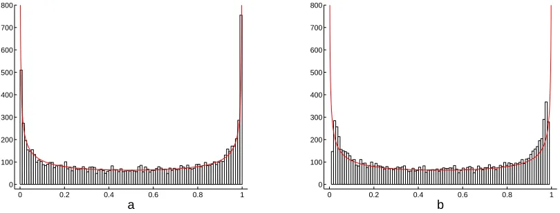
right, especially at moderate times T. No formal goodness-of-fit tests were applied, but the histograms in Figs.1and 2below clearly demonstrate the developingU-shape characteristic of the arcsine distribution, however with the speed of such a convergence apparently depending on the function f involved (and, of course, on the observation timeT used).

We start with the “canonical” case where the Heaviside function H(x) =1(0,∞)(x)

chosen representation of the histogram). As already mentioned, the noticeable differ-ence between the highest columns at the left and right edges may be attributed to asymmetry of the process Xt+. More precisely, the proportion of the sample values

of η_T+(0;H) falling, say, in the first box, ∆1 (from 0 to 0.01) and the last box, ∆100

(from 0.99 to 1) is given by 510 and 750, respectively, yielding the relative frequencies 510/10,000 = 0.051 and 750/10,000 = 0.075. The corresponding limiting probabilities, computed from the arcsine distribution (1.3), equal 0.064 for both ∆1 and ∆100 (here

and below, we give numerical values to two significant figures). This discrepancy can be quantified using the exact theoretical distribution ofη_T+(0;H) obtained in Theorem 2.1 (see formula (2.8) with T = 1 000), giving the probability 0.052 for ∆1 and 0.077

for ∆100, where the latter includes the atom 2ϕT(1) = 0.025. For comparison, with

a tenfold observation time T = 10 000, these probabilities become 0.060 and 0.068, respectively, with the atom much reduced, 0.008. It is also worth mentioning that, as indicated by these results, the fit with the limiting arcsine distribution would be much better for the “symmetric” versionηT(0;H) corresponding to the telegraph processXt

(see (1.5)).

0 0.2 0.4 0.6 0.8 1

0 100 200 300 400 500 600 700 800

a

0 0.2 0.4 0.6 0.8 1

0 100 200 300 400 500 600 700 800

b

Figure 1: Histograms for the occupation time functionalη+

T(0;f) with (a) the Heaviside step function

f =H and (b) the function f(x) =π−1_arctanx+1

2. The parameters of the telegraph process X + t

are standardized toc = 1 and λ= 1. Both histograms are obtained withN = 10,000 simulations, each over the observation timeT = 1 000. The length of each box on the histogram is ∆ = 0.01. The red solid curve represents the scaled arcsine density (i.e., multiplied byN∆ = 100).

The long-term prediction contained in a more general Theorem 2.4 was verified by computer simulations for the functional η_T+(0;f) with the probing functionf(x) = π−1_arctanx+1

2. The new histogram plot (see Fig. 1b), obtained with the same values

of c, λ, T and N, is qualitatively similar to that on Fig. 1a, including a small right bias, but convergence to the arcsine distribution becomes slower, apparently due to additional time needed for the process to explore the limiting valuesf_± of the function f at_±∞, which eventually determine the distributional limit.

Incidentally, this observation helps to understand the difference between the sets of hypotheses in Theorems 2.3 and 2.4; indeed, the additional condition of Theorem 2.4, requiring that c2_{T/λ → ∞ as T → ∞, guarantees a sufficient mobility of the}

from the origin. In contrast, if the functionf is reduced to the Heaviside step function H, the limiting values H₋= 0, H+= 1 are encountered by the process straight away,

so no extra mobility is needed.

Let us point out that the asymptotic condition (2.21) imposed in Theorem2.4on the probing functionfis rather strong, assuming the existence of the limits limx→±∞f(x) =

f_±. This is in contrast with the paper by Khasminskii [Kh99] mentioned in the In-troduction, where f is subject to the weaker condition limx→±∞ x−1R0xf(u) du = f±

(cf. (1.4)). Unfortunately, we were unable to reach the same level of generality; in particular, our proofs of formulas (7.12), (7.14) and the key Lemmas 7.1 and 7.2 (see Section7) are heavily based on condition (2.21).

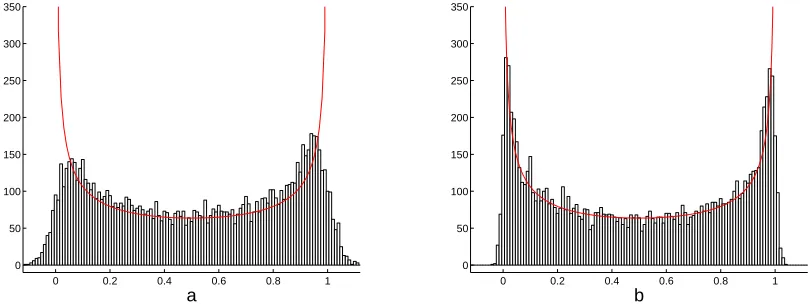
0 0.2 0.4 0.6 0.8 1 0

50 100 150 200 250 300 350

a

0 0.2 0.4 0.6 0.8 1 0

50 100 150 200 250 300 350

b

Figure 2: Histograms for the functionalη+T(0;f) with the probing function f(x) = π− 1_arctan

x+ cosx+ 1

2. The parameters of the telegraph process are as in Fig. 1, with the same number of runs

N= 10,000 and the observation time (a)T = 1 000 or (b)T = 10 000. Compare with Fig. 1 and note the improved quality of fit to the hypothetical arcsine distribution (red curve) on the right plot as compared to the left one.

However, we conjecture that Theorem 2.4 does hold under the weaker limiting condition (1.4) (see Remark 2.4). To verify this claim numerically, we carried out computer simulations for the distribution ofη+_T(0;f) withf(x) =π−1_{arctanx+cosx+} 1

2. Figure 2a shows the simulated histogram with the old values T = 1 000 and N =

10,000, which reveals a bimodal distribution but not quite well fit to the hypothetical arcsine limit; in particular, there are noticeable “parasite” shoulders outside the interval [0,1], which are indeed possible because the function f may take values less than 0 and bigger than 1. However, the fit with the arcsine shape significantly improves under longer observations, T = 10 000 (see Fig. 2b). In particular, the high modes at the edges are better pronounced, while the shoulders outside [0,1] are considerably reduced.

Appendix A. Probabilistic proofs of Theorems 2.2, 2.3 and 2.4

A.1. Theorem 2.2

in so doing the prior knowledge of the distribution ofη±_T(0) (provided by Theorem2.1) is essential.

Let us recall some information related to the first-passage problem for the telegraph process X_t±. For x < 0, let T±_−x := inf_{t _≥ 0 : X_t± = ₋x_} (with the convention that inf_∅:= +_∞) be the hitting time of point₋x >0 by the process X_t±(starting from the origin, X₀± = 0). If we set T0 := (−x)/c, then the distribution of T±₋x is concentrated

on [T0,∞) and is given by (see [Pi91, §0.5, pp. 12–13], [FK94, pp. 150–153] or [Or95,

Theorem 4.1, p. 18])

P{T+_{−x ∈}dt}= e−λT0_δ

T0(dt) +Q

+

−x(t) dt, P{T−−x∈dt}=Q−−x(t) dt, (A.1)

where the densities Q±₋x are defined exactly by equations (2.13), (2.14).

Consider the two-dimensional Markov process (X_t±, V_t±), where X_t± is the (condi-tional) telegraph process (1.6) (i.e., with the initial velocity V0 = ±c, respectively),

andVt± = dXt±/dt =±c(−1)Nt is the corresponding velocity process driven by a

Pois-son process Nt which determines the reversal instants of the motion Xt± (see (1.6)).

It is obvious that T±_−x is a stopping time for the process (X_t±, V_t±). Also note that Vt±

¯ ¯

t=T±_−x= +c (a.s), since the first passage through point−x >0 by the process X

±

t ,

starting from the origin, with probability 1 can only occur from left to right, that is, with positive velocity. Hence, conditioning on the hitting time of the origin starting fromx < 0 (which, of course, has the same distribution asT±_−x) and using the strong Markov property of the joint process (Xt±, Vt±), we have, for each y∈[0,1−T0/T],

P{η_T±(x)∈dy}=P{T±_−x > T}δ0(dy) +E

£

P{η±_T(x)∈dy, T0 ≤T±₋x≤T |T±−x}

¤

= µZ ∞

T P{

T±_{−x ∈}du}

¶

δ0(dy)

+

Z (1−y)T

T0

P{T±_{−x ∈}du_}P{(1₋u/T)η_T+_−u(0) _∈dy_}. (A.2)

Here, the first integral represents the case where the telegraph process Xt± does not

reach the origin before time T and, therefore, never enters the positive half-line (thus contributing to the atomδ0(dy)), while the second integral (where integration is taken

with respect to du) accounts for the first passage event (at time instant u ∈[T0,(1−

y)T]), so that the telegraph process, restarted from the origin (with the initial velocity +c), has to spend on the positive half-line the required timeTdy during the remaining travel time T −u.

In view of (A.1) together with (2.13) and (2.14), and due to equation (2.8) which provides the distribution ofη_T+_−u(0), formula (A.2) furnishes an explicit representation of the distribution of η_T±(x). On account of the atom in (A.1), the right-hand side of (A.2) specializes to

µZ ∞

T

Q±₋x(u) du

¶

δ0(dy) +µ±T(dy) +

Z (1−y)T

T0

Q±₋x(u) P

½

η_T+_−u(0) ∈ dy

1−u/T ¾

du,

whereµ−_T(dy) := 0 and

µ+_T(dy) := e−λT0

P

½

η_T+_−T0(0)∈ dy

1−T0/T

¾

. (A.4)

Using (2.8), for any u_∈[T0,(1−y)T] we have

P

½

η_T+_−u(0) _∈ dy 1−u/T

¾

= 2ϕT−u(1)δ1−u/T(dy) +ψT−u

µ y 1−u/T

¶ dy

1−u/T . (A.5)

Substituting (A.5) (with u=T0) into (A.4) readily gives (2.11), while the last term on

the right-hand side of (A.3) is reduced to (cf. (2.10))

2T Q±_−x((1₋y)T)ϕT(y) dy+

Z (1−y)T

T0

Q±_−x(u) µ

ψT−u

µ y 1₋u/T

¶ dy 1₋u/T

¶ du,

where the contribution of the atomδ1−u/T(dy) from (A.5) is easily computed via the

ob-vious symbolic formulaδ1−u/T(dy) du=T δ(1−y)T(du) dy. Indeed, for any test functions

F(y) and G(u) we have, by changing the order of integration,

Z 1−T0/T

0

F(y)

Z (1−y)T

T0

G(u)δ1−u/T(dy) du

= Z T

T0

G(u) du

Z 1−u/T

0

F(y)δ1−u/T(dy)

= Z T

T0

G(u)F(1−u/T) du

=T

Z 1−T0/T

0

F(y) Ã

Z (1−y)T

T0

G(u)δ(1−y)T(du)

!

dy.

A.2. Theorem 2.3

The idea of a probabilistic proof of Theorem 2.3 (as well as of Theorem 2.4, see AppendixA.3below) is based on the diffusion approximation of the telegraph process (see Theorem 1.1). More precisely, making the substitution t = T u and using that H(αx)_≡H(x) for any α >0, we can rewrite formula (2.1) as

η±_T(x) = Z 1

0

H(x+X_{T u}± ) du= Z 1

0

H(xT +Z_u,T± ) du, (A.6)

where xT := γT−1/2x, Zu,T± := γ−

1/2

T XT u±, and γT := c2T /λ. Note that (Zu,T± , u ≥ 0) is

a telegraph process with rescaled parameters λT := λT → ∞, cT := (λT)1/2 → ∞,

which therefore converges weakly to a standard Brownian motion (Bu, u ≥ 0) (by

Theorem 1.1). Hence, if xT → a as T → ∞ (cf. the hypotheses of Theorem 2.3) then

from (A.6) we immediately obtain the convergence in distribution

η_T±(x)_−→d h₁(a) := Z 1

0

According to (1.1) and (1.2), the random variableh1(0) has the arcsine distribution,

which proves Theorem2.3fora= 0. Fora <0 (so that₋a >0), letτ₋a := min{t ≥0 :

Bt=−a}be the hitting time of the point−aby the Brownian motionBtstarting from

the origin (B0 = 0). As is well known since P. L´evy’s paper [Le40, Th´eor`eme 2, p. 294]

(see also [IM74,_§1.7, p. 26] or [Fe71, _§VI.2(e), pp. 174–175]), the random variableτ₋a

has probability densityq₋a(·) defined in (2.15). Note thatτ−a is a stopping time (with

respect to the natural filtration_Ft :=σ{Bs, 0≤ s≤ t}). Conditioning on τ−a (when

a+Bτ−a = 0) and using the strong Markov property, we obtain, for any y∈[0,1],

P{h₁(a)_∈dy_}=_P{τ₋a >1}δ0(dy) +

Z 1−y

0

q₋a(u)P{(1−u)h1−u(0)∈dy}du

= µZ _∞

1

q₋a(u) du

¶

δ0(dy) +

µZ 1−y

0

q₋a(u)

1₋u pas µ

y 1₋u

¶ du

¶ dy,

which coincides with (2.17) (for Y₋a) in view of (2.18) and (2.19). Finally, the case

a >0 easily follows by the obvious symmetry relation h1(a)

d

= 1₋h1(−a) (cf. (2.3)).

A.3. Theorem 2.4

According to the proof of Theorem2.3, it suffices to establish an analogue of relation (A.7), that is,

η_T±(x;f)−→d h₁(a) = Z 1

0

H(a+Bu) du, T → ∞. (A.8)

Similarly to (A.6), rewrite formula (2.24) as

η_T±(x;f) = Z 1

0

f(x+X_{T u}± ) du= Z 1

0

f¡

γT(xT +Zu,T± )

¢ du,

whereγT, xT andZ_u,T± are the same as in Appendix A.2. In particular, if xT →athen

the process ˜Zu,T :=xT +Zu,T± weakly converges to the shifted Brownian motion a+Bu.

On the other hand, observing that γT →+∞ (by the hypothesis of Theorem2.4), we

havef(γTx)→H(x) for each x6= 0. Hence, it is natural to expect that

Z 1

0

f(γTZ˜u,T) du d

−→

Z 1

0

H(a+Bu) du, T → ∞, (A.9)

which is equivalent to (A.8).

To verify (A.9), let us represent the left-hand side of (A.9) as

Z 1

0

£

f(γTZ˜u,T)−H( ˜Zu,T)

¤ du+

Z 1

0

H( ˜Zu,T) du=: Ξ(1)T + Ξ

(2)