ON ERRORS-IN-VARIABLES ESTIMATION WITH UNKNOWN NOISE VARIANCE RATIO I. Markovsky∗,A. Kukush∗∗, andS. Van Huffel∗
∗ESAT, SCD-SISTA, K.U.Leuven, Kasteelpark Arenberg 10,
B-3001 Leuven, Belgium
∗∗Kiev National Taras Shevchenko University, Vladimirskaya st.
64, 01033, Kiev, Ukraine
Abstract: We propose an estimation method for an errors-in-variables model with un-known input and output noise variances. The main assumption that allows identifiability of the model is clustering of the data into two clusters that are distinct in a certain specified sense. We show an application of the proposed method for system identification.
Keywords: errors-in-variables, system identification, total least squares, clustering.
1. INTRODUCTION
Corresponding to the total least squares (TLS) prob-lem
{Rˆtls,Dˆtls}:=argmin R,Dˆ
D−Dˆ2
F subject to
RR=Ip and RDˆ =0 (1)
is the errors-in-variables (EIV) model
D=D¯+D,˜ rank(D) =¯ row dim(D)−p=:m. (2)
Here ¯Dis a true value and ˜Dis a measurement error that is modeled as a zero mean random matrix with in-dependent and identically distributed (i.i.d.) elements. The TLS estimator (1) is maximum likelihood for the EIV model (2) if, in addition to the previous assump-tions, the entries of ˜Di jare normally distributed. The variance of ˜Di j needs not be known, but the i.i.d. assumption is often too restrictive.
More general EIV models, where the measurement errors need not be i.i.d., have been considered in (Kukush and Van Huffel, 2004). The corresponding TLS-type problems are called weighted TLS prob-lems. A key assumption in this work is that the noise covariance structure, i.e., the covariance matrix of vec(D)˜ is known up to a scaling factor. One can argue that the knowledge of the noise covariance structure up to a scalar is again restrictive in practice.
EIV models with two or more unknown noise pa-rameters, however, are unidentifiable by second order methods, i.e., there are many solutions that are not distinguishable from the second order statistics. This unidentifiability problem is well known in the context of the Frisch scheme (Frisch, 1934; De Moor, 1988). For dynamical systems a similar negative result is first proven in (Anderson, 1985).
Various additional assumptions can be imposed in order to make the EIV estimation problem with un-known noise covariance structure identifiable. An overview of methods for EIV system identification is given in (Söderströmet al., 2002; Söderström, 1981). In this paper we show a new assumption that allows to derive consistent parameter and noise variance es-timates. The idea comes from (Wald, 1940), where a static single input single output (m=p=1) EIV model is considered and the proposed estimator is the line passing through the mean values of two clusters of data points. We develop this simple idea for multi input single output static and dynamic EIV models. The key consistency assumption for the method is that the dataDhas as many clusters as there are unknown noise parameters. For example, the proposed method is not applicable for problems where the inputs are stationary, which is a typical assumption in much of the prior work on EIV system identification. Also in
the dynamic case, we assume that the input and output measurement noises are white and uncorrelated.
The assumption that the data can be clustered means that the true input changes character while the noise properties remain the same. This assumption can be viewed equivalently as having a set of data records from experiments with different true inputs. Such an assumption is certainly restrictive and presently we do not have specific applications in mind.
In Section 2 we describe kernel and input/output representations of static and dynamic linear models. Section 3 presents the proposed estimation method for static EIV models and states conditions for con-sistency. Section 4 extends the method to dynamic models and Section 5 shows simulation examples for EIV system identification. For simplicity the proposed method is applied to the special case of single out-put models and covariance structure known up to two unknown scalars: the input and the output noise vari-ances. In the conclusions we discuss the extension of the method for problems involving more than two unknown parameters of the covariance matrix.
2. KERNEL AND INPUT/OUTPUT REPRESENTATIONS OF LINEAR MODELS
2.1 Static models
The data matrixD∈Rq×Nhas as rows the variables of interest and as columns the observed samples of those variables. A linear static modelBforDis a subspace ofRq. Such a model can be represented as the kernel of a matrixR∈Rg×q,i.e.,
B={d∈Rq|Rd=0}=: ker(R).
In the numerical linear algebra literature, however, the input/output representation
B(X):=
d=
di
do
m
p
Xdi=do
(3)
is preferred over the kernel one because it makes explicit the input/output structure of the model. The matrixX∈Rm×p,m+p=qinB(X)is a parameter of the model. Note that while the parameterRin a kernel representation is in general non-unique, for a fixed input/output partitioning, the parameterXis unique.
GivenR, one can always find ˜R, such that ˜RR˜=Ip and ker(R˜) =ker(R). Note that ifRis full row rank, then the number of rowsg:=row dim(R)ofRis equal to the number of outputs p of B=ker(R). In the single output case,RR=R2=1, makesRunique.
The firstmvariablesdi in the input/output
represen-tation (3) are inputs,i.e., they can be chosen freely. The lastpvariablesdoare outputs,i.e., they are fixed
by the input and the model. The integers m and p are invariant of the representation. Note that not ev-ery modelB⊆Rqadmits an input/output represen-tation with a fixed input/output partitioning. The set
of models that can not be represented in the form (3), however, is non-generic inRq.
Corresponding to the representation (3) are the in-put/output partitionings of the data and measurement error matrices
D=:
Di
Do
m
p and D˜ =:
˜ Di
˜ Do
m
p. In Section 3 we use the input/output representation (3) and assign different noise variances to the input and output variables.
2.2 Dynamic models
In the dynamic context the given datawd∈(Rq)T is a
finite vector time series and the model is a subset of the data space (Rq)T. We consider linear time-invariant (LTI) models. The LTI model class admits a difference equation representation
B(R):={w∈(Rq)T |R0w(t) +R1w(t+1) +···
+Rlw(t+l) =0, fort=0,...,T−l}. (4) The matricesRi∈Rg×qare parameters of the model. Withg=1 andRl=0,B(R)is a single output model. A given LTI model B generically admits an in-put/output representation
B=
w=
u y
m
1
P0y(t) +P1y(t+1) +···
+Ply(t+l) =Q0u(t) +Q1u(t+1) +···
+Qlu(t+l), fort=0,...,T−l
,
Pi∈Rp×p,Qi∈Rp×m, and
∑l
k=0Pkzk −1
∑l k=0Qkzk is a proper rational function (transfer function ofB).
3. STATIC PROBLEMS WITH ONE OUTPUT AND TWO UNKNOWN NOISE PARAMETERS
First we consider the special case of EIV static model with one output and covariance structure known up to two scalars: input and output noise variances. This model corresponds to the classical linear system of equationsAx≈bwith noises onAandbof unknown size. The model is unidentifiable without additional information on the noise covariance structure. For example, the weighted TLS method requires that the ratio of the input and output noise variances is known.
Our assumption about the noise covariance matrix is that
ED˜D˜=
ED˜iD˜i ED˜iD˜o
ED˜oD˜i ED˜oD˜o
=:
¯
λiWi 0
0 λ¯oWo
, (5)
where Wi∈Rm×m and Wo∈R are known positive
definite matrices, and ¯λi (the input variance) and ¯λo
Provided that the smallest eigenvalue of the sam-ple covariance matrixDDhas multiplicity one (the generic case), the TLS solution ˆRtls is unique and is
given by the eigenvector ofDD, corresponding to the smallest eigenvalue. Alternatively, we are looking for a solutionRto the nonlinear system of equations
R(DD−λI) =0 corresponding to the smallest value ofλ.
The TLS solution corresponds to an EIV model, in which the input/output noise variance ratio
¯
λi/λ¯o=: ¯μ
is equal to one,{D˜i,i j}are i.i.d., and{D˜o,i j}are i.i.d.
The case of aknownnoise ratio ¯μ=1, corresponds to a weighted TLS problem, which seeks for a solution to the system
R
DD−λo
¯
μIm 0 0 1
=0,
corresponding to the smallest value ofλo. The
numer-ical solution in this case is performed via the gen-eralized eigenvalue or singular value decomposition (instead of the ordinary eigenvalue or singular value decomposition).
Denote
W(μ):=
μWi 0
0 Wo
,
so thatED˜D˜=λ¯oW(μ¯). Corresponding to the EIV
model and assumption (5) is the weighted TLS prob-lem
min
ˆ
R,D
W−1/2(μ¯)(D−D)ˆ 2
F subject to R
ˆ D=0,
or equivalently the nonlinear system of equations
R
DD−λoW(μ¯)
=0, (6)
where again the true input/output noise ratio ¯μ is as-sumed known. The computation can be carried out via a generalized eigenvalue or singular value decom-position. In the literature the estimator for this case is called generalized TLS (Van Huffel and Vande-walle, 1989).
Now consider the problem of unknown true noise ra-tio ¯μ. Even ifRis properly normalized,e.g.,R=1, a solution to (6) is non-unique. This is a manifestation of a lack of identifiability of the model with unknown input and output noise variances. We propose to re-solve the unidentifiability problem by considering a system of two independent estimating equations. After a permutation of the columns ofDvia a permutation matrixΠ, define
DΠ=:D1 D2=:
D1i D2i
D1o D2o
m
1
and consider two copies of (6)
R
Dk(Dk)−λoW(μ)
=0, fork=1,2, (7) corresponding to the two partsD1andD2of the data matrix.
If the minimal singular value ofD1
i(D1i)−D2i(D2i)
is separated from zero, the problem of estimating si-multaneouslyλo,μ, andR is identifiable (see
Theo-rem 1 below). This condition is related to the existence of clusters in the true data ¯D. Correspondingly the clustering problem is
max
permutation matrixΠ
min j=1,...,m
λj
D1i(D1i)−D2i(D2i)
, (8) whereλ1(A),...,λdim(A)(A)are the eigenvalues ofA.
The estimation problem corresponding to (7) is more complicated than a generalized eigenvalue/singular value decomposition: we need to find a common gen-eralized eigenvalue-eigenvector pair for two pairs of symmetric positive semidefinite matrices that depend on a scalar parameter. In general, (7) has no exact solution, so that an approximation is needed.
We propose the following nonlinear least squares type approximate solution:
ˆ
μ=argmin μ
λ1 o−λo2
2
+Csin2∠(R1,R2) , (9) where(λk
o,Rk)is the minimal generalized
eigenvalue-eigenvec. pair of the pencilDk(Dk),diag(μW
i,Wo) ,
Cis a regularization parameter, and∠(R1,R2)stands for the angle between the vectors R1 and R2. The first term in the cost function makes both eigenval-ues close to each other, while the second term makes the corresponding eigenvectors close to each other. The regularization parameterCallows to turn the two objectives optimization problem into a one objective optimization. Our experience is that the results are rather insensitive to the value of this parameter and in the simulation examples of Section 5 we setC=1.
Once the optimal estimate ˆμ of the noise variance ratio μ is found, the estimation problem becomes a classical generalized TLS problem. In summary, the proposed estimation procedure has three stages.
1. Cluster the data by solving (8).
2. Compute the noise variance ratio estimate ˆμby solving (9) for the clusters identified on step 1. 3. Solve the standard generalized TLS problem for
the estimated value ofμon step 2.
The clustering problem (8) has combinatorial com-plexity, so that (except for small examples) it can be solved only via heuristic methods. See (Xu and Wun-sch, 2005) for a survey of clustering algorithms. In our simulation examples we use the K-means algorithm implemented in the Statistics Toolbox of MATLAB.
The optimization problem on step 2 is a rather simple one because it involves a single scalar decision vari-able and the search interval is lower bounded by 0. Note that each cost function evaluation involves two generalized singular value decompositions.
In (Kukushet al., 2005), steps 2 and 3 of the algorithm are different.
2’. Compute the noise variance estimates ˆλiand ˆλo
by solving the optimization problem
min λi,λo
μ1
μ2
2+Csin2∠(R1,R2)
, (9’)
where μk and Rk are respectively the smallest eigenvalue and corresponding eigenvector of
Dk(Dk)−diag(λiWi,λoWo).
3’. Define the estimate ˆRas the eigenvector corre-sponding to the smallest eigenvalue of the matrix
DD−diag(λˆiWi,λˆoWo).
Problem (9) can be viewed as a modification of (9’). In general both problems are nonconvex and non-smooth, however, (9) is univariate while (9’) is bi-variates and for this reason more difficult to solve. The estimator on Step 3’ is called the adjusted least squares. It is equivalent to the generalized TLS esti-mator on step 3 with ˆμ=λˆi/λˆo.
Statistical consistency of the estimator using steps 2’ and 3’ is proven in (Kukushet al., 2005). Here we state the main result, specialized for the considered problem. (The result of (Kukushet al., 2005) applies to multi input multi output dynamic problems as well.)
Theorem 1. Assume that:
i). there existsδ >0, such thatE|D˜i j|4+δ are uni-formly bounded for alli,j
ii). N1 1
¯
D1iF and N1
2 ¯
D2iF are bounded, where
N1:=col dim(D1)andN2:=col dim(D2)
iii). lim infN1,N2→∞σmin 1
N1D
1
iD1i −N12D
2
iD2i >0,
whereσmin(A)is the smallest singular value ofA,
iv). lim infN1→∞
1
N1trace(X
W iX)>0
lim infN2→∞
1
N2trace(Wo)>0, and v). lim infNk→∞
1
Nkσmin
¯
Dki(D¯ki) >0, fork=1,2. Then ˆλi→λ¯i, ˆλo→λ¯o, and ˆX →X, as¯ N1,N2→∞,
almost surely.
4. APPLICATION FOR DYNAMIC MODELS
Certain system identification problems can be posed as structured TLS problems (Markovskyet al., 2005a). The main difference with the static TLS problem (1) is that now the data matrix is block-Hankel struc-tured. For application of the structured TLS method, however, the measurement error covariance structure should be known up to a scaling factor. In this sec-tion we address a dynamic version of the problem of Section 3.
Written in a matrix form the difference equation
R0w(t) +R1w(t+1) +···+Rlw(t+l) =0,
becomes the structured system of equations
RHl+1(w) =0, (10)
whereHl+1(w)is the block-Hankel matrix withl+1 block rows, constructed from the time seriesw:
Hl+1(w):= ⎡ ⎢ ⎢ ⎢ ⎣
w(1) w(2) ··· w(T−l) w(2) w(3) ··· w(T−l+1)
w(3) w(4) ··· w(T−l+2) .
. .
. . .
. . .
w(l+1) w(l+2) ··· w(T) ⎤ ⎥ ⎥ ⎥ ⎦, (11)
and
R:=R0 R1 ··· Rl
.
With noisy data wd and T >q(l+1) +l,
generi-cally (4) is not compatible, so that an approximation is needed.
The structuredTLS problem is the dynamic equiva-lent of the TLS problem (1):
min
R,wˆ w−wˆ 2
subject to RR=1,
and RHl+1(w) =ˆ 0. (12)
Its solution however can not be expressed in closed form via a singular value decomposition of the data matrix as in the static case and needs nonlinear opti-mization methods (Markovskyet al., 2004).
The structured TLS problem (12) corresponds to the EIV model wd=w¯+w, where ¯˜ w is a trajectory of
B(R)¯ for some ¯R∈R1×q(l+1), and ˜wis a white random
sequence with covariance matrix that is equal to a multiple of the identity. If in addition the measurement errors ˜ware normally distributed, the structured TLS estimator is maximum likelihood.
More generalweighted structured TLSproblems allow to take into account the noise covariance matrix that is known up to a scaling factor. As in the static case, dynamic EIV problems in which the covariance struc-ture is specified up to more than one scaling factor are unidentifiable.
Next we consider the case when the noise covariance matrix is known up to two scalars—the input and output noise variances. Accordingly,
covw˜(t) = ¯
λiIm 0 0 λ¯o
=λ¯o
¯
μIm 0 0 1
=: ¯λoW(μ¯).
(13) Let
W(μ):=diag(W (μ),...,W (μ) Ttimes
).
The weighted structured TLS problem corresponding to the EIV model with the noise covariance (13) is
min
R,wˆ (wd−w)ˆ
W−1(μ¯)(w
d−w)ˆ subject to
RR=1, RHl+1(w) =ˆ 0. (14)
However, this problem can be solved only for a given parameter ¯μ.
is generically equivalent to the following nonlinear weighted least squares problem
min X
X −1Hl+1(wd)Γ−1(X,μ¯)Hl+1(wd)
X
−1
(15) whereΓ(X,μ¯)is a block banded and Toeplitz matrix that depends onX andW(μ¯). In turn the optimiza-tion problem (15) can be seen equivalently as a least squares approximate solution method for the nonlinear system of equations
X −1Hl+1(wd)Γ−1/2(X,μ¯) =0.
In order to resolve the identifiability problem, we make the assumption that the true time series ¯w changes its behavior at timeT,i.e., the time series
¯
w1:= (w(1),...,¯ w(T¯ ))
has different mean and dispersion than the time series
¯
w2:= (w(T¯ +1),...,w(T¯ )).
This assumption corresponds to the clustering as-sumption in the static case. Note that now the ordering of the data samples corresponds to time, so that we can not permute them as in the static case.
Under the existence of clusters, define w1d, w2d anal-ogously to ¯w1, ¯w2, and consider the system of two nonlinear equations
Xk −1Hl+1(wkd)Γ−1/2(X,μ) =0, fork=1,2.
(16) For noise free data, the equations have a common solution X1=X2=X¯ and μ =μ¯. In the presence of noise, an approximate solution is needed and we propose the same criterion as in the static case
ˆ
μ=arg min μ
λ1 o−λo2
2
+Csin2∠(R1,R2) , (17) whereRkandλokcome from the structured TLS
prob-lems associated with (16),
Rk:=(Xk) −1, and
λk
o:=RkHl+1(wkd)Γ−1(X,μ)Hl+1(wkd)(Rk).
Each cost function evaluation involves solving two structured TLS problems.
In summary, the algorithm for the considered EIV identification problem is:
1. Detect a time instantTat whichwdchanges its
behavior.
2. Solve the optimization problem (17) for the par-titioning of the data found in step 1, and 3. Solve the structured TLS problem (14) for the
estimated value ˆμin step 2.
Note 1. The cost functions in (9), (9’), and (17) are discontinuous. Therefore, the global minimum might not exist. The minimization is performed up to certain tolerance that decreases to zero, as the number of observations increases.
5. SIMULATION EXAMPLE
Consider the EIV model (2). The covariance structure of the measurement errors ˜D is known up to scal-ing factors (the true noise variances) ¯λi and ¯λo. The
simulation example aims to show consistency of the estimators for the unknown parameters ¯λi, ¯λo, and ¯X,
the parameter in an input/output representation of the true model that has generated the data ¯D.
LetUN(l,u)be a matrix withNcolumns, composed of independent and uniformly distributed random vari-ables in the interval[l,u]. The true values ¯Diand ¯Rare
selected as follows:
¯ Di=
UN(−0.5,0.5)UN(10,20)
, X¯=1 1, whereN is varied from 10 to 500. Correspondingly
¯
Do:=X¯D¯i. Note that we artificially create two
clus-ters (the firstNand the lastNcolumns of ¯D). In this simulation example the K-means clustering algorithm detects without errors the two clusters. The measure-ment errors are zero mean, independent, normally dis-tributed with variancesλi=0.01 andλo=0.04.
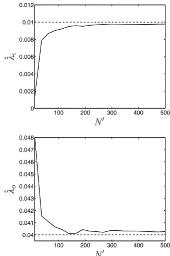
With this simulation setup we apply the proposed estimation method and average the results for 500 noise realizations. The average values of the noise variance estimates ˆλiand ˆλoare shown on Figure 1.
Figure 2 shows the average relative estimation error
e:= 1 500
500
∑
k=1X¯−Xˆ(k)
X¯ ,
where ˆX(i)is the estimate of the parameter ¯Xin theith repetition of the experiment.
100 200 300 400 500
0 0.002 0.004 0.006 0.008 0.01 0.012
N
ˆλi
100 200 300 400 500
0.04 0.041 0.042 0.043 0.044 0.045 0.046 0.047 0.048
N
[image:5.595.323.493.480.735.2]ˆλo
Fig. 1. Average values of the noise variance estimates ˆ
λiand ˆλoas a function of half the sample sizeN.
100 200 300 400 500 0
0.002 0.004 0.006 0.008 0.01 0.012 0.014 0.016
N
[image:6.595.99.258.68.190.2]e
Fig. 2. Relative error of estimationeas a function of half the sample sizeN.
6. CONCLUSIONS
We have considered an EIV estimation problems for single output static and dynamic systems, with mea-surement error covariance matrix known up to two unknown parameters. The model is identifiable under the assumption that the data has two clusters that are distinct in a specified sense. The proposed estimation method has three steps: cluster the data, solve a uni-variate optimization problem for the noise variance ratio, solve a standard TLS-type problem for the es-timated noise variance ratio. In the static case the cost function evaluation on the second step involves solv-ing a couple of generalized TLS problems and in the dynamic case it involves solving a couple of weighted structured TLS problems.
Identifiability of the model is recovered by construct-ing two estimatconstruct-ing equations correspondconstruct-ing to the two clusters. The idea generalizes to problems involv-ing more than two unknown parameters in the mea-surement error covariance matrix. As many clusters and corresponding estimating equations are needed as there are unknown covariance parameters. The estima-tion procedure in this case, however, requires solving a multidimensional optimization problem on the second step. It is an open problem what special properties (if any) this optimization problem has and how to exploit them in effective EIV estimation algorithms.
ACKNOWLEDGEMENTS
I. Markovsky is a postdoctoral researcher and S. Van Huffel is a full professor at the K.U.Leuven, Belgium. A. Kukush is a full professor at the Kiev National Taras Shevchenko Univ., Ukraine. We are grateful to Prof. H. Schneeweiss for fruitful discussions. Prof. Kukush is supported by a senior postdoctoral fellowship from the Dep. of Applied Economics of the K.U.Leuven. Our research is supported by Research Council KUL: AMBioRICS, GOA-Mefisto 666, several PhD/postdoc & fellow grants; Flemish Gov-ernment: FWO: PhD/postdoc grants, projects, G.0078.01 (struc-tured matrices), G.0407.02 (support vector machines), G.0269.02 (magnetic resonance spectroscopic imaging), G.0270.02 (nonlinear Lp approximation), G.0360.05 (EEG signal processing), research communities (ICCoS, ANMMM); IWT: PhD Grants; Belgian Fed-eral Science Policy Office IUAP P5/22 (‘Dynamical Systems and
Control: Computation, Identification and Modelling’); EU: PDT-COIL, BIOPATTERN, ETUMOUR.
REFERENCES
Anderson, B. (1985). Identification of scalar errors-in-variables models with dynamics.Automatica 21, 625–755.
De Moor, B. (1988). Mathematical concepts for mod-eling of static and dynamic systems. PhD thesis. Dept. EE, K.U.Leuven, Belgium.
Frisch, R. (1934). Statistical confluence analysis by means of complete regression systems. Technical Report 5. Univ. of Oslo, Economics Institute. Kukush, A. and S. Van Huffel (2004). Consistency
of elementwise-weighted total least squares esti-mator in a multivariate errors-in-variables model AX=B.Metrika59(1), 75–97.
Kukush, A., I. Markovsky and S. Van Huffel (2005). Estimation in a linear multivariate measument error model with clustering in the re-gressor. Technical Report 05–170. Dept. EE, K.U.Leuven.
Markovsky, I. and S. Van Huffel (2005). Weighted structured total least squares. Technical Report 05–41. Dept. EE, K.U.Leuven.
Markovsky, I., J. C. Willems, S. Van Huffel, B. De Moor and R. Pintelon (2005a). Application of structured total least squares for system identifi-cation and model reduction.IEEE Trans. on Aut. Control50(10), 1490–1500.
Markovsky, I., S. Van Huffel and A. Kukush (2004). On the computation of the structured total least squares estimator. Num. Lin. Alg. with Appl. 11, 591–608.
Markovsky, I., S. Van Huffel and R. Pintelon (2005b). Block-Toeplitz/Hankel structured to-tal least squares. SIAM J. Matrix Anal. Appl. 26(4), 1083–1099.
Söderström, T. (1981). Identification of stochastic lin-ear systems in presence of input noise. Automat-ica17(5), 713–725.
Söderström, T., U. Soverini and K. Mahata (2002). Perspectives on errors-in-variables estimation for dynamic systems. Signal Processing 82, 1139– 1154.
Van Huffel, S. and J. Vandewalle (1989). Analysis and properties of the generalized total least squares problemAX ≈B when some or all columns in A are subject to error. SIAM J. Matrix Anal. 10(3), 294–315.
Wald, A. (1940). The fitting of straight lines if both variables are subject to error.Ann. Math. Stat. 11, 284–300.