Model predictive control for Active Bridge Active Clamp (ABAC) converter

Model Predictive Control for an Active-Bridge-Active-Clamp

(ABAC) Converter

Linglin Chen*_{, Luca Tarisciotti}*_{, Alessandro Costabeber}*_{, Davide Gottardo}*_{, Pericle Zanchetta}*_{, and Pat Wheeler}*

*Department of Electrical and Electronics Engineering, University of Nottingham, Nottingham, UK. E-mail: [email protected]

Keywords: DC/DC converter, Active-Bridge-Active-Clamp (ABAC), Model Predictive Control (MPC).

Abstract

The Dual-Active-Bridge is a well-established isolated, bidirectional DC/DC topology suitable for applications where high efficiency, galvanic isolation and large voltage conversion ratios are required. However, in low voltage high power cases, the output current ripple is significant and large filtering capacitance is needed. As an alternative to the standard Dual-Active-Bridge, the Active-Bridge-Active-Clamp (ABAC) converter is presented in this paper. The ABAC converter overcomes the current ripple limitation of Dual Active Bridge by presenting a current interleaved structure. An average switching model is developed for the ABAC converter by neglecting the dynamic on the high frequency link, and a Model Predictive Control (MPC) is proposed. The control features a reduced prediction horizon and a fixed switching frequency. Finally, simulation results for a 10kW ABAC converter are provided to validate the theoretical claims.

1 Introduction

Recently, there has been a great research interest in topics related to More Electric Aircraft (MEA) [1–4]. In MEA, electrical systems are used to replace hydraulic or pneumatic sources [5]. The Boeing 787 and the Airbus A380 both have considerably larger electrical system than any previous aircrafts [6], with 1MW and 600kVA power capacity respectively. A number of different voltage standards exist for the electrical system on large civilian aircraft [7]. For example, 28VDC for powering avionics and other loads, 270VDC for power transmission, and 115VAC generated from Starters/Generators (S/G) are often present in the aircraft electrical system. In the DC distribution, power converters interfaced with 270VDC High-Voltage (HV) and 28VDC Low-Voltage (LV) may be required. Considering that energy storages and Fuel cells can be installed on the 28VDC link [6] galvanic isolation and bi-directional power flow are essential for DC/DC converters used in this application.

Dual-Active-Bridge (DAB) has a great potential in this application for its high power conversion efficiency and power controllability [6, 29]. However, one of the issues with DAB is the current harmonics on both HV and LV side. Therefore, extra filters are required [8, 9] to prevent current harmonics from propagating into HV and LV DC networks Large current harmonics may also cause voltage resonance in

presence of long power cable as investigated in [10]. In order to overcome these issues, several current-fed DAB topologies have been proposed in [11–14], where current smoothing inductors can be configured to either AC [11, 12] or DC side [13] of the LV full bridge. However, current-fed solution in [11, 12] cannot achieve complete ripple cancellation over the full operation range, while the topology in [13] requires high voltage rated semiconductor devices. Lastly, authors in [14] proposed an input-output paralleled topology which increases the required number of active devices.

When fast dynamic controllers are required, Model Predictive Control (MPC) is an attractive solution which provides several advantages, such as easy inclusion of nonlinearities and constraints, fast dynamics and simple digital implementation [15]. In particular, Finite Control Set Model Predictive Control (FCS-MPC) has been intensively investigated in AC power conversion [15, 17, 19] such as inverters, rectifiers, active filters and uninterruptible power supplies. The applications of MPC in DC/DC converters are reported in [16, 18, 20–22]; The authors in [16] propose the implementation of FCS-MPC in a boost converter with the receding horizon. However this approach results in a larger current ripple than a PI-PWM based approach with the same sampling rate. In [18, 21], authors have compared a Continuous Control Set MPC (CCS-MPC) with a hysteresis control in a boost converter. Although the dynamics performances are similar in the two control approaches, the voltage overshoot is completely avoided by using CCS-MPC control. In [20] a single step prediction CCS-MPC is implemented, together with an outer PI loop to regulate the output voltage of a buck converter. This shows better response performance than a PI-PWM based control. The authors in [22] include switching loss and transformer current Root-Mean-Square (RMS) value into the cost function, and evaluate among different modulations. This approach can achieve optimal efficiency throughout the operation range, but the dynamic performance remains the same with the PI control approach.

approach considers the dynamic on the high frequency link by taking into account the DC component of the transformer current [24]. A generalized discrete small signal modelling method for resonant converters is proposed in [25], based on Taylor’s series and state plane diagram. Alternatively, matrix exponential linearization technique is employed in [26] for deriving the discrete time model. Lastly, authors in [28] concludes that similar modelling accuracy can be achieved by using both discrete time modelling and average modelling which neglects the dynamic on the high frequency link. Active-Bridge-Active-Clamp (ABAC) converter [29], shown in Fig. 1, is introduced in this paper. Similarly to the DAB. The ABAC converter can be intuitively modulated with conventional Single Phase Shift (SPS) modulation. The average modelling is obtained by neglecting the dynamics on the high frequency link and, based on this model, a MPC is proposed for the ABAC converter. Steady state oscillations are suppressed by introducing the output current variation constraints and variable prediction range.

This paper is organized as follows: in Section 2, the ABAC converter topology is introduced, and operation with SPS is provided. In Section 3, a switching average model for the ABAC converter is provided. In Section 4, MPC is proposed for the ABAC converter. Simulation results in Section 5 are presented for a 10 kW ABAC converter.

2 ABAC with SPS

The schematic of the ABAC converter topology is presented in Fig. 1. It is composed of a full bridge, associated to the higher voltage side of the converter, connected to the primary of the high frequency transformer.

vC1

+ -vINCin

T1 T3

T4

T2

-vac1

n:1

+

iL1

T5

+ -vo

Lo1

RL

Co

Ls

vac2

iO1 ILV

T6

Ls

T7

T8

T9

T10 T11

T12

iL2

Lo2

iL3

Lo3

iL4

Lo4

iO

iO2

+

-vac3

+

-C3

C1

C2

C4 +

-vC2 +

-vC3 +

-vC4 +

-is1

is2

RLi

Rline1

Rline2

IHV

VHV

VLV

iI

[image:2.595.364.492.457.632.2]

T Fig. 1 The topology of ABAC.

Two interleaved half bridge clamp circuits are connected to each of the two windings on the secondary sides of the transformer. In general, the two secondary circuits can operate independently. However, for the proposed analysis, interleaved operation will be assumed, in order to minimize load current ripple. In Fig. 1, vac1 and vac2 are transformer

primary and upper secondary voltages respectively. The lower secondary voltagevac3is controlled to be the same asvac2in

order to perform even current sharing.LsandRsrepresent the

transformer leakage impedance at the secondary side, providing the required energy storage necessary to control power transfer from primary to secondary and vice-versa.C1 -C4 are the clamping capacitors which serve as a buffer

between the transformer and LV load. Lo1-Lo4are the output

filter inductors which are used to reduce the output current

angle φ between the primary and each of the secondary voltages is controlled to transfer power while producing 50% duty cycle waveforms on each side of transformer. To generate theses waveforms, the HV H-Bridge (T1 to T4) is

switched across its active states without applying any zero vectors. Similarly, on the LV converter side, leg 1 (T5, T6)

and 2 (T7, T8) are complementarily switched, synchronous

with leg 3 (T9, T10) and leg 4 (T11, T12), respectively.

Typical waveforms of such modulation applied to the ABAC converter are shown in Fig. 2, wherevac1andvac2have a 50%

fixed duty cycle and the phase shift φ is imposed. Representative gating signals are also shown in Fig. 2, with

G1 toG12 driving the switches from T1 to T12, respectively.

The output currents iL1-iL4 are controlled by the switching of

the LV stage T5-T12. In each of the LV side legs, if the upper

switch is turned on, the correspondent output current increases, since the clamping voltages vc1-vc2are higher than

the output capacitor voltage vO. For the same reason, if the

lower switch is on, the output current decreases. In Fig. 2, during intervalθ1-θ3, T5and T9are on, resulting in the linear

increase ofiL1andiL3. At the same time, since T8and T12are

also on, iL2 andiL4 decrease. When considering equal output

inductors, complete current ripple cancellation can be achieved between iL1 andiL2, as well as between iL3 andiL4.

Note that iC1 is the current flowing from power transferring

inductor (Ls) into the clamp capacitor (C1), and iLc1 is the

current flowing from clamp capacitor (C1) to the output

inductor (Lo). The difference betweeniC1andiLc1is equal to

the current provided by the clamp capacitor (C1), and in

steady state operation, its average value is equal to zero. A similar behaviour can be appreciated during the intervalθ3-θ4,

resulting in a pure DC output current.

vac2

G5

G7

G9

G11

iL1

iL2

φ

 vac1

iL4

iL3

θ θ θ θ θ θ

G1

θ

θ1 θ2θ3 θ4

is1

θ

θ iI

 

 



iC1 iLc1

φ1

[image:2.595.47.287.462.544.2]

φ2

Fig. 2 Theoretical waveforms for ABAC modulated with SPS (φ=φ1=φ2).

From top to bottom are transformer primary voltagevac1, secondary voltage

vac2, secondary transformer currentis1, output currentsiL1-iL4, HV side input

currentiI, currents flowing through clampC1, driving signalsG1-G11.

3 Modelling

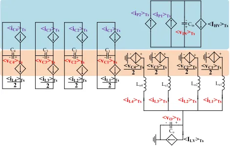
general switching average model that works for all modulations [30–33] can be readily derived as shown in Fig. 3 where state variables (<vIN>Ts, <vO>Ts, <vC1>Ts, <iL1>Ts,

etc.) are highlighted in red. On the other hand the controllable current sources (<iC1>Ts, <iP1>Ts,etc…) are highlighted in

violet, and their produced waveform presents different shapes, accordingly to the modulation applied. Finally the HV and LV currents,<IHV>Tsand<ILV>Tsonly depends on source

and load conditions.

<iP2>Ts<iP1>Ts

<iC4>Ts <iC3>Ts <iC2>Ts <iC1>Ts

<vC1>Ts

<vC3>Ts

<vC4>Ts <vC2>Ts

Cin + -+ -+ -+ -Lo1 Lo2 Lo3 Lo4 Co

<iL1>Ts

<iL2>Ts

<iL3>Ts

<iL4>Ts

+ -C1 + -C2 + -C3 + -C4 +

-<v_-O>+Ts

<vC1>Ts

2 <vC2>Ts

2 <vC3>Ts

2 <vC4>Ts

2 <iL1>Ts

2 <iL3>Ts

2 <iL22>Ts <iL4>Ts

2

<ILV>Ts

[image:3.595.50.285.190.342.2]

<IHV>Ts <vIN>Ts

Fig. 3 The averaged model of the ABAC converter

The state-space equations are illustrated in (1). The notation

<x>Ts indicates the average value of x calculated over a

switching period. Expressions for currents <iC1>Ts-<iC4>Ts,

<iP1>Ts, and <iP2>Ts depend on the different modulations

applied to the ABAC converter, which will be addressed later.

4 1 1 2 1 1 2 1 1 2 1 1

1 1 1

( 1, 2,3, 4) s s s s s s s s s s

s s s

Cm T

Lm T Cm T

m m

Lm T

Cm T O T

om om

O T

Lm T LV T

m

o o

IN T

HV T P T P T

in in in

d v

i i

dt C C

d i

v v

dt L L

d v

i I

dt C C

d v

I i i

dt C C C

m              _{ }  _{     }      _{     }                



(1)

Considering the case where both HV and LV side are connected to ideal stiff voltage sources VHV andVLV, thus

assuming that the line impedances are small enough to be neglected (Rline1=Rline2=0). In this case, state-space equation

(1) can be modified into (2), resulting in the output equations of (3). With symmetrical parameters (Lo1=Lo2=Lo3=Lo4=Lo, C1=C2=C3=C4=C) and SPS modulation, the expression for <iCm>Tsis provided in (4) [34], under the assumption that the

clamp voltage is constant in one switching cycle.

1 2 1 1 2 1 1 2

( 1, 2,3, 4)

s

s s

s

s s

Cm T

m Lm T Cm T

Lm T

m Cm T LV T

o o

d v

f i i

dt C C

d i

f v V

dt L L

m                          (2) 1 2 3 4 1 2 3 4

(0 0 0 0 1 1 1 1) s s s s s s s s s C T C T C T C T O T L T L T L T L T v v v v i i i i i     _{ }    _{ }    _{ }                _{ }    _{ }    (3)

(1 ) ; 1, 2,3, 4

4 s

s

Cm T HV

s

T

i V m

nL

   

     (4)

In (4), n is the transformer turn ratio; Ts is the switching

period; VHV is the input voltage; Ls is the sum of secondary

leakage and power transferring inductance; φ is phase shift between primary and secondary voltage square waves. Using this model, a PI controller, which is considered as term of comparison for the MPC, is designed. Since, equation (4) shows nonlinearity, linearization of equation (4) is conducted around the equilibrium operating point.

^

s T

x x x

    (5)

where, x is the equilibrium point; x^ is the small signal

perturbation.. Therefore, the state-space equation (2) can be linearized as follows

~ ~

1 1 _~

~ ~ 1 1 / / C C L L

d v dt v

A B

d i dt i 

                            (6) where 11 11 1 1 21 21 1 1 | |

; 1, 2,3, 4

| |

1

0 0 0 0 0 0 0

2 1

0 0 0 0 0 0 0

2 1

0 0 0 0 0 0 0

2 1

0 0 0 0 0 0 0

2 1

0 0 0 0 0 0 0

2 1

0 0 0 0 0 0 0

2 1

0 0 0 0 0 0 0

2 1

0 0 0 0 0 0 0

2 cm Lm s s cm Lm s s v i

c T L T

v i

c T L T

o o o o f f v i

A _{f f} m

11 21

1/ 1/ 1/

( | | ) 1/

0

0

 

   

 

 

 

  _{ }

 

   

 

 

 

 

 const

C C C

f f

B K C (8)

andKconstis a constant value:

2 2

s HV const

s

T V K

nL

  (9)

As a result, equations (3), (6)-(8) describe a small signal state-space model for the ABAC converter using the SPS modulation. However, the state-space model developed above only considers the ideal transformer without coupling between the upper secondary and the lower secondary.

4 Proposed MPC

The aim of the designed MPC controller is to regulate the output current iO in Fig. 1 at the desired reference value.

Instead of using the small signal model in (7) and (8), the

averaged model of (2) is considered,

2 1

1 1

2 2

2

2 2

2 2

3

3 3

2 2

4

4 4

2

1 1

4 2

1 1

4 2

1 1

4 2

1 1

4 2

  

      

 

 



      



 _{ }

 _{      }



 _{ }

 _{      }



s

s s

s

s s

s

s s

s

s s

L T

L T C T

o o

L T

L T C T

o o

L T

L T C T

o o

L T

L T C T

o o

d i

i i

L C L C

dt d i

i i

L C L C

dt d i

i i

L C L C

dt d i

i i

L C L C

dt

(10)

obtaining for the output current, which is the sum of the four equations in (10) the following expression

2

2

1 _{(1 )}

4 2

   

 

     

s

s

O T s

O T HV

o s o

d i T

i V

L C nL L C

dt (11)

Equation (11) is then discretized using numerical approximation [35] as follows

1 2 3

[ ] [ ]

[ 1]  [ ]  [ 1]  (1  )

 

     

O O O HV

k k

i k i k i k V (12)

where,λ1,λ2andλ3are constant values

2

1

2 3

3 2

4 1

2

   

   

   

  

s

o

s

o s

T CL

T nCL L

(13)

Therefore, to predict the output current value at time k+1, only phase shift value at timekand sampled output currents at both timekandk-1are required. The cost function for the MPC controller is then defined as

2 2

1( [ 1] [ 1]) 2( [ 1] [ ])

 

 _oref  _o   _o  _o

ct i k i k i k i k (14)

where,ioref[k+1]is the output current reference value;α1and

second term is introduced for its ability of reducing steady state output current oscillation.

The phase shift required to minimise the defined cost function is obtained by considering a variable control output range- In fact, as the phase shift can change from -90° to 90°, and a control precision (the smallest phase shift value that can be controlled) of Δd degree is assumed, a total number of

Ne=180/ Δd points need to be evaluated during every

sampling interval, which is usually not feasible within one switching period in practical experiment. Alternatively, in one sampling period, only a number of 2Npre+1 points are

assessed around operating phase shiftφ[k-1]as shown in (15).

Npreis related to the number of iteration which the controller

is required to evaluate during every sampling interval.

[ ] [ 1] ( ) ( 0 2 )

 k  k  i N_pre _d i _ N_pre (15) Assumingφop_{[k] is the outcome of the minimization of cost}

function (14). CurrentiOop[k+1]is the estimated current value

by takingφop_{[k]into (12). WheniO}op_{[k+1]gets closer to the}

reference ioref[k+1], the estimation range Npre reduces, as in

(16)

* [ 1] [ 1]

[ 1]

  





op

oref O

pre pre

oref

i k i k

N N

i k (16)

where, 2Npre* is related to the maximum evaluation time for

the cost function. Therefore, the value is subjected to the computational power of the practical digital platform. By using this variable prediction range algorithm, the steady state oscillation on transformer current can be largely reduced, as shown in simulation.

5 Simulations

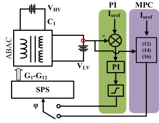
The MPC controller is designed and implemented in simulation software PSIM as illustrated in Fig. 4. The PI controller is also designed based on system small signal model (7). Only output current is measured and controlled and the output of both controllers is considered to be the phase shift in SPS modulation. This phase shift is then fed into SPS modulation, generating the driving signalsG1-G12.

SPS G1-G12

VLV Ioref -VHV

PI C1

A

B

A

C

Ioref

(12) (14) (16)

PI MPC

[image:4.595.348.505.563.685.2]

φ

Fig. 4 The control diagram of the ABAC converter

ValuesNpre*=10 and Δd=0.36 (in degree) are assumed in the

ABACCONVERTER SIMULATION PARAMETERS

Symbol Description Value

VHV HV voltage 270V

VLV LV voltage 28V

Pm Rated power 10 kW

fs Switching frequency 100 kHz

n Transformer turn ratio 5

Co Output capacitor 24 uF

C Clamp capacitors 150 uF

Ls Power transfer inductors 500 nH

Rs Secondary series resistors 1mΩ

Lo Output inductors 3.3 uH

Ro Output stray resistors 5mΩ

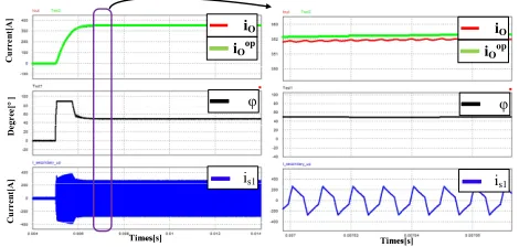
The simulation results on MPC are shown in Fig. 5 when the weighing factor α2=0 the variable prediction range is

disabled, and thus Npre=Npre*. The green dots in the figure

illustrate the predicted output current. It shows perfect match with the simulated output current. Therefore, the model (12) is validated. Large oscillation on output current, phase shift and transformer current are observed. This is due to the fact that one step prediction cannot guarantee overall performance over long period of time.

iO

C

u

rr

en

t[

A

]

φ

D

eg

re

e[

°

]

C

u

rr

en

t[

A

] i_s1

Times[s]

iOop

iO

φ

is1

iOop

[image:5.595.310.545.117.229.2]

Times[s]

Fig. 5 The simulation on MPC when the weighing factorα2=0 and Npre=Npre*.

The waveforms from top to bottom are output currentio, phase shift valueφ

and upper secondary transformer currentis1

The MPC controller is improved by putting an output current variation constraint into the cost function as illustrated in (14). The weighing factors are tuned empirically. The simulation results for the weighing factorsα1=0.05,α2=1are

shown in Fig. 6 with the variable prediction range still disabled. It can be observed that the oscillation on output current is significantly reduced, but there still exists oscillations on phase shift and transformer current at steady state. This may reduce the power conversion efficiency.

iO

C

u

rr

en

t[

A

]

φ

D

eg

re

e[

°

]

C

u

rr

en

t[

A

] is1

Times[s]

iOop

iO

φ

is1

iOop

Times[s] 300

200 100 0 -100

100 80 60 40 20 0

600 400 200 0 -200 -400

400 354

352

350

100 80 60 40 20 0

500

[image:5.595.57.277.326.426.2]

-500 0

Fig. 6 The simulation on MPC when the weighing factorsα1=0.05,α2=1and

Npre=Npre*. The waveforms from top to bottom are output current io, phase

shift valueφand upper secondary transformer currentis1

The final proposed MPC control (with both current variation constraint and variant estimation range applied) is simulated and results are shown in Fig. 7. It can be noted that

oscillations in phase shift, transformer currents and output current are well suppressed.

iO

C

u

rr

en

t[

A

]

φ

D

eg

re

e[

°

]

C

u

rr

en

t[

A

] is1

Times[s]

iOop

iO

φ

is1

iOop

Times[s]

Fig. 7 The simulation on MPC when the weighing factorsα1=0.05,α2=1,and

variant estimation range is applied. Waveforms from top to bottom are output currentio, phase shift valueφand upper secondary transformer currentis1

Comparison between using proposed MPC and PI controller has been carried out in Fig. 8. It can be noted in Fig. 8 (b) there is no overshoot in output current. The settling time for MPC is only 1.8ms. However in Fig. 8 (a), overshoot is still present when similar settling time are considered for both controllers. In this case, settling time for the PI controller is 5ms, which is higher than the one obtained using the proposed MPC controller.

iO

C

u

rr

en

t[

A

]

φ

D

eg

re

e[

°

]

C

u

rr

en

t[

A

] _i

s1

Times[s]

5ms

iO

φ

is1

1.8ms

Times[s]

(a) (b)

Fig. 8 Dynamic (0kw to 10kw) comparison for (a) PI and (b) MPC controlled ABAC. The waveforms from top to bottom are output currentio[100A/div],

phase shift value φ[20°/div] and upper secondary transformer currentis1

[200A/div]

6 Conclusions

In this paper, a MPC algorithm is proposed for the control of the ABAC converter. The proposed method can increase the dynamic performances of the ABAC converter. Moreover, with the proposed method more constraints can be added to the cost function, enabling more advanced modulation patterns which improves the converter performances in different operating conditions.

Simulations on a 10-KW ABAC converter have been conducted to verify the theoretical claims. The effectiveness of the proposed MPC is validated and the effectiveness of the imposed current constraints and variable prediction range is proven. In fact, steady state oscillations are clearly reduced using the proposed MPC. Comparison between proposed MPC with the PI controller is also carried out. The proposed method shows faster dynamic than the PI controller.

[image:5.595.311.543.362.473.2] [image:5.595.46.277.571.680.2]

excessively increase the computational burden on the control hardware.

References

1 Nagel, N.: ‘Actuation Challenges in the More Electric Aircraft: Overcoming Hurdles in the Electrification of Actuation Systems’IEEE Electrif. Mag., 2017,5, (4), pp. 38–45.

2 Jia, Y., Rajashekara, K.: ‘Induction Machine for More Electric Aircraft: Enabling New Electrical Power System Architectures’IEEE Electrif. Mag., 2017,5, (4), pp. 25–37. 3 Ngoua Teu Magambo, J.S., Bakri, R., Margueron, X., et al.:

‘Planar Magnetic Components in More Electric Aircraft: Review of Technology and Key Parameters for DC–DC Power Electronic Converter’IEEE Trans. Transp. Electrif., 2017,3, (4), pp. 831–842. 4 Xu, Q., Wang, P., Chen, J., Wen, C., Lee, M.Y.: ‘A Module-Based Approach for Stability Analysis of Complex More-Electric Aircraft Power System’IEEE Trans. Transp. Electrif., 2017,3, (4), pp. 901– 919.

5 Wheeler, P., Bozhko, S.: ‘The More Electric Aircraft: Technology and challenges.’IEEE Electrif. Mag., 2014,2, (4), pp. 6–12. 6 Buticchi, G., Costa, L., Liserre, M.: ‘Improving System Efficiency

for the More Electric Aircraft: A Look at dc\/dc Converters for the Avionic Onboard dc Microgrid’IEEE Ind. Electron. Mag., 2017, 11, (3), pp. 26–36.

7 Tariq, M., Maswood, A.I., Gajanayake, C.J., Gupta, A.K.: ‘Aircraft

batteries : current trend towards more electric aircraft’IET Electr. Syst. Transp., 2017,7, (2), pp. 93–103.

8 Pugliese, S., Mastromauro, R.A., Stasi, S.: ‘270V/28V wide bandgap device-based DAB converter for more-electric-aircrafts: Feasibility and optimization’, in ‘2016 International Conference on Electrical Systems for Aircraft, Railway, Ship Propulsion and Road Vehicles & International Transportation Electrification Conference (ESARS-ITEC)’ (IEEE, 2016), pp. 1–6

9 Zhang, K., Shan, Z., Jatskevich, J.: ‘Large- and Small-Signal Average-Value Modeling of Dual-Active-Bridge DC–DC Converter Considering Power Losses’IEEE Trans. Power Electron., 2017,32, (3), pp. 1964–1974.

10 Riedel, J., Holmes, D.G., McGrath, B.P., Teixeira, C.: ‘Active Suppression of Selected DC Bus Harmonics for Dual Active Bridge DC–DC Converters’IEEE Trans. Power Electron., 2017, 32, (11), pp. 8857–8867.

11 Shi, Y., Li, R., Xue, Y., Li, H.: ‘Optimized Operation of Current-Fed Dual Active Bridge DC&amp;#x2013;DC Converter for PV Applications’IEEE Trans. Ind. Electron., 2015,62, (11), pp. 6986– 6995.

12 Zhang, J., Sha, D.: ‘A current-fed dual active bridge DC-DC converter using dual PWM plus double phase shifted control with equal duty cycles’, in ‘2016 Asian Conference on Energy, Power and Transportation Electrification (ACEPT)’ (IEEE, 2016), pp. 1–6 13 Bal, S., Rathore, A.K., Srinivasan, D.: ‘Comprehensive study and analysis of naturally commutated Current-Fed Dual Active Bridge PWM DC/DC converter’, in ‘IECON 2016 - 42nd Annual Conference of the IEEE Industrial Electronics Society’ (IEEE, 2016), pp. 4382–4388

14 Shi, J., Zhou, L., He, X.: ‘Common-Duty-Ratio Control of Input-Parallel Output-Input-Parallel (IPOP) Connected DC–DC Converter Modules With Automatic Sharing of Currents’IEEE Trans. Power Electron., 2012,27, (7), pp. 3277–3291.

15 Kouro, S., Cortés, P., Vargas, R., Ammann, U., Rodríguez, J.: ‘Model predictive control—A simple and powerful method to control power converters’IEEE Trans. Ind. Electron., 2009,56, (6), pp. 1826–1838.

16 Karamanakos, P., Geyer, T., Manias, S.: ‘Direct model predictive current control of DC-DC boost converters’, in ‘2012 15th International Power Electronics and Motion Control Conference (EPE/PEMC)’ (IEEE, 2012), p. DS2c.11-1-DS2c.11-8

17 Tarisciotti, L., Zanchetta, P., Watson, A., Bifaretti, S., Clare, J.C.: ‘Modulated Model Predictive Control for a Seven-Level Cascaded

K.: ‘MPC of Switching in a Boost Converter Using a Hybrid State Model With a Sliding Mode Observer’IEEE Trans. Ind. Electron., 2009,56, (9), pp. 3453–3466.

19 Tarisciotti, L., Zanchetta, P., Watson, A., Clare, J.C., Degano, M., Bifaretti, S.: ‘Modulated Model Predictive Control for a Three-Phase Active Rectifier’IEEE Trans. Ind. Appl., 2015,51, (2), pp. 1610–1620.

20 Liu, K.Z., Yokozawa, Y.: ‘An MPC-PI approach for buck DC-DC converters and its implementation’, in ‘2012 IEEE International Symposium on Industrial Electronics’ (IEEE, 2012), pp. 171–176 21 Kinoshita, H., Liu, K.Z., Zaharin, A., Yokozawa, Y.: ‘High

performance algorithms for the control and load identification of boost DC-DC converters’, in ‘2010 IEEE Vehicle Power and Propulsion Conference’ (IEEE, 2010), pp. 1–6

22 Yade, O., Gauthier, J.-Y., Lin-Shi, X., Gendrin, M., Zaoui, A.: ‘Modulation strategy for a Dual Active Bridge converter using Model Predictive Control’, in ‘2015 IEEE International Symposium on Predictive Control of Electrical Drives and Power Electronics (PRECEDE)’ (IEEE, 2015), pp. 15–20

23 Rodriguez, A., Vazquez, A., Lamar, D.G., Hernando, M.M., Sebastian, J.: ‘Different Purpose Design Strategies and Techniques to Improve the Performance of a Dual Active Bridge With Phase-Shift Control’IEEE Trans. Power Electron., 2015,30, (2), pp. 790– 804.

24 Xiangli, K., Li, S., Smedley, K.M.: ‘Decoupled PWM Plus Phase-Shift Control for a Dual-half-bridge Bidirectional DC-DC Converter’IEEE Trans. Power Electron., 2017, pp. 1–1.

25 Batarseh, I., Siri, K.: ‘Generalized approach to the small signal modelling of DC-to-DC resonant converters’IEEE Trans. Aerosp. Electron. Syst., 1993,29, (3), pp. 894–909.

26 Shi, L., Lei, W., Li, Z., Huang, J., Cui, Y., Wang, Y.: ‘Bilinear Discrete-Time Modeling and Stability Analysis of the Digitally Controlled Dual Active Bridge Converter’IEEE Trans. Power Electron., 2017,32, (11), pp. 8787–8799.

27 Hengsi Qin, Kimball, J.W.: ‘Generalized Average Modeling of Dual Active Bridge DC–DC Converter’IEEE Trans. Power Electron., 2012,27, (4), pp. 2078–2084.

28 Krismer, F., Kolar, J.W.: ‘Accurate Small-Signal Model for the Digital Control of an Automotive Bidirectional Dual Active Bridge’IEEE Trans. Power Electron., 2009, 24, (12), pp. 2756– 2768.

29 Tarisciotti, L., Costabeber, A., Linglin, C., Walker, A., Galea, M.: ‘Evaluation of isolated DC/DC converter topologies for future HVDC aerospace microgrids’, in ‘2017 IEEE Energy Conversion Congress and Exposition (ECCE)’ (IEEE, 2017), pp. 2238–2245 30 Naayagi, R.T., Forsyth, A.J., Shuttleworth, R.: ‘Performance

analysis of extended phase-shift control of DAB DC-DC converter for aerospace energy storage system’, in ‘2015 IEEE 11th International Conference on Power Electronics and Drive Systems’ (IEEE, 2015), pp. 514–517

31 Huang, J., Wang, Y., Li, Z., Lei, W.: ‘Unified Triple-Phase-Shift Control to Minimize Current Stress and Achieve Full Soft-Switching of Isolated Bidirectional DC–DC Converter’IEEE Trans. Ind. Electron., 2016,63, (7), pp. 4169–4179.

32 Bal, S., Yelaverthi, D.B., Rathore, A.K., Srinivasan, D.: ‘Improved Modulation Strategy using Dual Phase Shift Modulation for Active Commutated Current-fed Dual Active Bridge’IEEE Trans. Power Electron., 2017, pp. 1–1.

33 Xu, G., Sha, D., Zhang, J., Liao, X.: ‘Unified Boundary Trapezoidal Modulation Control Utilizing Fixed Duty Cycle Compensation and Magnetizing Current Design for Dual Active Bridge DC–DC Converter’IEEE Trans. Power Electron., 2017,32, (3), pp. 2243–2252.

34 Alonso, A.R., Sebastian, J., Lamar, D.G., Hernando, M.M., Vazquez, A.: ‘An overall study of a Dual Active Bridge for bidirectional DC/DC conversion’ (2010), pp. 1129–1135