Numerical modelling of transient liquid phase bonding and other diffusion controlled phase changes

J O U R N A L O F M A T E R I A L S S C I E N C E 4 0 (2 0 0 5 ) 2505 – 2511

Numerical modelling of transient liquid phase

bonding and other diffusion controlled

phase changes

T. C. ILLINGWORTH∗, I. O. GOLOSNOY, V. GERGELY, T. W. CLYNE

Department of Materials Science, University of Cambridge, Pembroke Street, Cambridge, CB2 3QZ, UK

E-mail: [email protected]

Diffusion in material of inhomogeneous composition can induce phase changes, even at a constant temperature. A transient liquid phase (TLP), in which a liquid layer is formed and subsequently solidifies, is one example of such an isothermal phase change. This

phenomenon is exploited industrially in TLP bonding and sintering processes. Successful processing requires an understanding of the behaviour of the transient liquid layer in terms of both diffusion-controlled phase boundary migration and capillarity-driven flow.

In this paper, a numerical model is presented for the simulation of diffusion-controlled dissolution and solidification in one dimension. The width of a liquid layer and time to solidification are studied for various bonding conditions. A novel approach is proposed, which generates results of a high precision even with coarse meshes and high interface velocities. The model is validated using experimental data from a variety of systems, including solid/solid diffusion couples. C 2005 Springer Science + Business Media, Inc.

1. Introduction

Transient liquid phases (TLPs) are observed in many al-loy systems. However, commercial exploitation of the phenomenon is relatively limited. This is partly because current understanding of the process is incomplete, ren-dering the optimisation of various process variables and design parameters difficult.

Qualitatively, TLPs are easily understood; a full de-scription of the underlying physical processes has been given by MacDonald and Eagar [1]. The essential re-quirement is that the liquidus temperature of an alloy varies with composition. It is then possible for variation of concentration in an inhomogeneous alloy to cause lo-calised melting at temperatures where the bulk of the material remains solid. If liquid and solid of different compositions are in contact, diffusion will change the concentration profile and can cause an initial widen-ing of the liquid layer, followed by solidification, even during an isothermal heat treatment. Such diffusion-controlled solidification can be used to bond particles in a powder compact (TLP sintering) or to join larger objects (TLP bonding).

Once solidified, the final composition in the vicinity of a joint can be relatively homogenous. As a result, its properties (such as strength and remelt temperature) can approach those of the parent material. The tran-sient presence of a liquid phase also affords advantages over other joining techniques. Flow under the influence of capillary forces will naturally tend to eliminate any

∗Author to whom all correspondence should be addressed.

porosity within a bond, without the need to impose any external pressure. In the case of TLP sintering, the liq-uid phase can additionally promote particle rearrange-ment, leading to rapid densification of a green body.

The transience of the liquid phase arises due to changes in composition which are a result of diffusion. In the next section, the physical processes which un-derlie TLPs are examined and a model is developed in which they are simulated.

2. Modelling

2.1. Mathematical description of the problem

Diffusion in both liquid and solid is assumed to be gov-erned by Fick’s second law (the “Diffusion Equation”),

∂c(x,t)

∂t =

∂ ∂x

D(c(x,t))∂c(x,t)

∂x

, (1)

where the composition, c(x,t), is a function of both position (x) and time (t). D(c(x,t)) is the diffusion coefficient of solute in either the liquid or solid phase, which depends on both temperature and concentration. The diffusion Equation 1 has been solved for a range of initial and boundary conditions. However, TLPs have solid and liquid phases which change size over time; this introduces a moving boundary condition, which complicates the analysis.

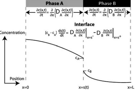
Figure 1 Schematic diagram showing the concentration profile across

a TLP bond at one instant in time. Only half of the joint is shown; the other half (from x= −L to x=0) will be symmetrical.

A one dimensional planar geometry is assumed, as shown in Fig. 1. The variable s(t) is introduced to de-scribe the position of a solid/liquid interface (which varies as a function of time). The moving boundary problem can then be expressed as [2]:

∂c(x,t)

∂t =

∂ ∂x

DA(c(x,t))∂

c(x,t)

∂x

, 0<x<s(t) (2)

∂c(x,t)

∂t =

∂ ∂x

DB(c(x,t))∂

c(x,t)

∂x

, s(t)<x<L (3)

DA(c(x,t))∂

c(x,t)

∂x

x₌s(t)−−

DB(c(x,t))∂

c(x,t)

∂x

x₌s(t)+

=[cB−cA]

ds(t)

dt . x =s(t) (4) The first equation describes diffusion to the left of the interface, in phase A (liquid in the case of Fig. 1). The second equation refers to diffusion in phase B, to the right of the interface (the solid). The third describes the moving boundary condition at the interface. It can be derived by assuming there is local equilibrium there, and by requiring solute conservation. (The notation cA

and cB is used for the equilibrium liquidus and solidus

concentration.) A complete statement of the problem also requires initial conditions, as well as conditions at the fixed boundaries x = 0 and x = L; these are triv-ial and are omitted for clarity. Any diffusion-controlled isothermal phase change with a planar geometry will obviously be subject to these governing equations, irre-spective of whether the phases are solid or liquid. The model developed below can thus be applied to solid state transformations, as well as TLPs.

Systems of partial differential equations with moving boundary conditions (also known as Stefan problems) arise in a variety of modelling situations across the sci-ences [3]. For certain idealised cases, analytical solu-tions are available [3–5]. In general, however, numer-ical solution methods are required. Several viable ap-proaches have been proposed. Unfortunately, Furzeland [6] concludes that the most effective approach to solv-ing a Stefan problem depends on the exact nature of the problem itself. Zhou et al. [7] describe numerical meth-ods formulated specifically to study TLP problems.

2.2. Fixed spatial discretisation models In modelling TLPs, the main difficulty arises in track-ing the motion of solid/liquid interfaces. Previously, a fixed discretisation of the domain x = 0 to x = L has generally been imposed, and a certain concentra-tion is associated with each point after every timestep. The motion of the interface can then be described in a number of ways.

One approach, used by Nakagawa et al. [8] and Cain et al. [9], is to solve the diffusion equations by impos-ing the requirement that the interface be located at one of the discretisation points. In this case, only a step-wise motion of the interface is permitted. Such a con-straint is physically unrealistic. In addition, restrictions on the interface position probably introduce significant errors into the model, as inaccurate approximations of the interface position will directly affect estimates of the fluxes there (and will therefore also affect the pre-dicted interface motion).

More refined models explicitly take account of the in-terface position and use a discretised form of Equation 4 to predict its motion. Shinmura et al. [10] used an al-gorithm based on this approach to investigate possi-ble interlayer materials for bonding nickel. Zhou and North [2] also employed this approach. In an attempt to improve the accuracy of their predictions for the in-terface motion, they additionally proposed the use of a quadratic expression for the concentration profile near the interface, in order to better estimate the fluxes there. These two models differ slightly in the way that they solve the diffusion Equations 2 and 3: Shinmura et al. [10] use an explicit expression, whereas Zhou and North [2] claim to use an implicit scheme. Cer-tainly, they solve an implicit form of Equations 2 and 3. However, the three Equations 2–4 are interdependent— implicit methods of calculating future concentration profiles will therefore give rise to expressions involv-ing future interface positions as well as future concen-trations. Since their method calculates future interface positions by solving (4) explicitly, their scheme is only semi-implicit overall. As a result, there is a limitation on the size of timestep that can be used to generate a solution.

Sinclair et al. [11] also implemented an explicit ver-sion of this same algorithm and used it to investigate the solidification of ternary systems. TLP bonding of sys-tems with three components has been investigated in parallel by Campbell and Boettinger [12]. They used generic software, which was developed to describe general diffusion-controlled transformations (not TLP bonding specifically).

Unfortunately, rapid interface motion is typical of the early stages of TLP bonding. Calculations using large timesteps will therefore contain inaccuracies associated with the non-conservation of solute. Eliminating these errors by reducing the step size has the drawback of increasing the computational effort required to solve the problem. The way in which the accuracy of predic-tions is affected by any particular choice has nowhere been addressed. In comparison, truncation errors are the only source of inaccuracy for conservative discreti-sation schemes.

2.3. Use of variable spatial discretisation Instead of ‘tracking’ the motion of a moving bound-ary across a fixed spatial discretisation, one alternative is to use a mesh which varies in a way that takes ac-count of the moving interface [3]. It is then possible to ensure that the interface position always coincides with a discretisation point without constraining its mo-tion. This approach was used by Tanzilli and Heckel to model solid-state phase transformations as long ago as 1968 [13]. Kajihara and Kikuchi [14] implemented an implicit version of the same model to investigate the behaviour of solidγ/α/γ diffusion couples in the Fe-Cr-Ni system.

In the present work, a variable space grid is achieved by introducing a wholesale co-ordinate transforma-tion using two new positransforma-tional variables: u= _s(t)x and

v= x−s(t)

L−s(t). These definitions mean that, for any time,

the interval 0 < x < s(t) coincides with 0< u < 1, and that s(t) < x < L coincides with 0 < v < 1. Changing co-ordinate system also means that the gov-erning Equations 2–4 must be modified. Writing p(u,t) as the concentration in phase A (which takes the same value as c(x,t) in 0 < x < s(t)) and q(v,t) as the concentration in phase B (corresponding to c(x,t) in s(t)<x < L), Equations 2–4 become [3]:

s(t)2∂p(u,t)

∂t −us(t)

ds(t) dt

∂p(u,t)

∂u

= ∂

∂u

DA( p(u,t))∂

p(u,t)

∂u

, 0<u<1 (5)

[L−s(t)]2∂q(v,t)

∂t −(1−v)[L−s(t)]

ds(t) dt

∂q(v,t)

∂v

= ∂

∂v

DB(q(v,t))

∂q(v,t)

∂v

, 0< v <1 (6)

DA( p(u,t))

s(t)

∂p(u,t)

∂u

u=1

− DB(q(v,t))

L−s(t)

∂q(v,t)

∂v

v=0

=[cB−cA]

ds(t)

dt . u=1; v=0 (7) In this new co-ordinate system, the interface is fixed at u=1 andv= 0 for all t. Fixing the front in this way means that interface motion can be handled more easily. On the other hand, the derivation of a finite difference scheme that conserves solute becomes more involved.

Using the identities ∂( pu)_∂u = p+u∂_∂p_u and

∂( ps)

∂t = p

ds dt +s∂

p

∂t, Equation 5 can be re-written

as

∂(ps)

∂t = ds dt

∂( pu)

∂u + 1 s

∂ ∂u

DA∂

p

∂u

. 0<u<1 (8)

Similarly, (6) can be expressed as

∂(q[L−s])

∂t = ds dt

∂(q(1−v))

∂v

+ 1

L−s

∂ ∂v DB ∂q ∂v

. 0< v <1 (9)

Discretising the space co-ordinate u at N points (u0. . .uN−1), writing ui±1/2 as the position midway

between ui and ui±1 and introducing the timestep δt

such that tj+1 _{= t}j _{+δt, the finite volume technique}

[15] is used to integrate the divergent form (8) over one spacestep and one timestep:

ui+1/2

ui−1/2

tj+1

tj

∂

∂t{ps}dtdu = tj+1

tj

ui+1/2

ui−1/2

∂ ∂u

×

ds dt pu+

DA

s

∂p

∂u

dudt. 0<u<1 (10)

Introducing p_ij+σ(and sj+σ_{) to represent the}

concentra-tion at ui(and the interface position) after a proportion

σ of the timestep has elapsed, Equation 10 leads to the approximation

p_ij+1sj+1− p_ijsj(ui₊1_/2−ui₋1_/2)

= δt sj+σ

(DA)

j_+σ i+1/2

p_ij₊+₁σ −p_ij+σ

ui+1−ui

−(DA)

j_+σ i−1/2

p_ij+σ− p_ij₋+₁σ ui−ui−1

+sj+1−sj

×p_ij₊+₁σ_/2ui+1/2− p

j+σ i−1/2ui−1/2

, (11)

where (DA)ij±+1σ/2 correspond to the diffusion

coeffi-cients for the concentrations mid-way between discreti-sation points. In the remainder of this work, diffusion coefficients will be assumed to be independent of con-centration. For a fixed bonding temperature, (DA)ij_±+1σ_/2

will be then be constant, taking a value which will be denoted DA.

Setting i = 1. . .N −2, Equation 11 can be used to generate a set of finite difference approximations for the future compositions in phase A. For i =0 or N−1, finite difference approximations for the relevant bound-ary conditions must be applied. At the moving interface (u =1), local equilibrium requires that p_Nj+₋1₁=cA. At

the fixed boundary (u = 0), standard techniques [15, 16] can be used to modify (11) so as to ensure zero flux. Doing so gives rise to the finite difference expression

p₀j+1sj+1−p₀jsj(u1/2)

= DAδt

sj+σ

p₁j+σ−p₀j+σ u1

+sj+1−sjp₁j_/+₂σu1/2

Similarly, integration can be used to generate finite dif-ference expressions for future compositions in phase B from Equation 9:

q_ij+1(L−sj+1)−q_ij(L−sj)(vi+1/2−vi−1/2)

= δt

L−sj+σ DB

q_ij₊+₁σ−q_ij+σ

vi+1−vi

−DB

q_ij+σ−q_ij₋+₁σ

vi−vi−1

+sj+1−sjq_ij₊+₁σ_/2(1−vi+1/2) −q_ij₋+σ_1/2(1−vi−1/2)

. (12)

Appropriate boundary conditions are easily derived in the same way as for phase A.

It remains to discretise Equation 7, which describes the motion of the interface and which follows from the requirement that solute be conserved there. A finite difference form can be derived in the same way. Ifvis discretised at M−1 points, the total amount of solute in the system at time tj+1is

sj+1

p₀j+1u1−u0 2 +

N−2

i=1

p_ij+1ui+1−ui−1 2

+p_Nj+₋1₁uN−uN−1 2

+(L−sj+1)

q₀j+1v1−v0 2

+ M−2

i=1

q_ij+1vi+1−vi−1 2 +q

j+1 M−1

vM−vM−1

2

.

A similar expression gives the total amount of solute at time tj. For the model to be conservative, the dif-ference between these two values must be zero. Sub-tracting one from the other gives rise to terms such as ui+1−ui−1

2 [s

j+1_pj+1

i −s j_pj

i], for which alternative

forms have been derived (Equations 11 and 12). Mas-sive cancellation upon substitution leaves only

DBδt

L−sj+σ

q₁j+σ−cB

v1

− DAδt

sj+σ

cA− p_Nj+₋σ₂

1−uN₋2

=sj+1−sj1+uN−2 2 p

j+σ

N−1−1/2+

1−uN₋2

2 cA

−

1− v1 2

q₁j_/+₂σ −v1 2cB

. (13)

Equations 11–13 form a finite difference formulation of the problem described analytically in Equations 5– 7. The way in which they were derived has ensured that they conserve solute. Appropriate approximations for terms at intermediate times (j+σ) and intermediate positions (i±1/2) will be considered presently, along with efficient methods of solving the resulting set of equations.

2.4. Implementation

The problems relating to diffusion ((11) and (12)) and interface motion (13) are interdependent: the diffusion equations involve the future interface position;

con-versely, for all implicit schemes (σ =0), the interface equation involves terms which depend on future con-centrations. The concentration profiles and the interface motion therefore form a strongly coupled problem. It follows that the equations cannot be solved indepen-dently; instead, they must be solved simultaneously.

Since the system of simultaneous equations is non-linear, an iterative solution method must be used. This is potentially very demanding in terms of computing time. But careful analysis can significantly improve the efficiency of the algorithm.

Firstly, note that it is trivial to solve Equation 13 for sj+1 if estimates are available for sj+σ and con-centration profiles p_ij+σ and q_ij+σ (from which inter-mediate concentrations p_ij_±+₁σ_/2and q_ij_±+₁σ_/2can be deter-mined). Once sj+1 _{has been calculated, it is easy to}

find future concentrations p_ij+1: assuming that terms such as p_ij_±+₁σ_/2 can be approximated sufficiently well using only the concentrations of neighbouring points at the same time (i.e. p_ij₋+₁σ,p_ij+σand p_ij₊+₁σ), Equation 11 is reduced to a tridigonal form, which can be inverted cheaply. Concentrations in phase B can also be calcu-lated by inverting a tridiagonal matrix which follows from (12).

Having decoupled and linearised the problem in this way, implementation is simple. The results discussed in the following section have been generated by an algo-rithm which, at each timestep, executes the following procedure:

(1) Take sj_,pj i and q

j

i as initial values for sj+σ,p j+σ i

and q_ij+σand calculate intermediate concentration pro-files p_ij₊+₁σ_/2and q_ij₊+₁σ.

(2) Calculate the future interface position, sj+1_using

(13).

(3) Using this value of sj+1_{, update the estimate for}

sj+σ_.

(4) Calculate the future interface positions, p_ij+1and q_ij+1 for all i using (11), (12) and the boundary conditions.

(5) Using these values for p_ij+1and q_ij+1, update the estimates for p_ij+σand q_ij+σand calculate intermediate concentration profiles p_ij₊+₁σ_/2and q_ij₊+₁σ_/2.

Steps (2)–(5) are then repeated until successive es-timates of the interface position sj+1 differ by less than some fixed tolerance. If successive refinements do indeed converge to some fixed value, this will cor-respond to a solution of the implicit set of discretised equations.

It is well known [16, 17] that the Crank-Nicolson scheme (σ = 1/2) gives an error that is propor-tional toδt2_{. This would seem preferable the fully}

im-plicit scheme (σ =1), which generates errors propor-tional toδt. However, if the Crank-Nicolson scheme is used to discretise discontinuous composition pro-files, unphysical oscillations will be predicted close to the discontinuity unless the timestep is of the or-der of _max(Dh2

is chosen [15–17]. Since discontinuous concentration profiles and large diffusion coefficients are inherent to TLPs, attention will be limited to fully implicit schemes.

Monotonicity concerns must also be taken into ac-count when considering possible approximations for the intermediate concentrations p_ij_±+₁σ_/2and q_ij_±+₁σ_/2. It is known that second-order centre-difference schemes can produce non-monotonic (oscillating) solutions [15, 17]. In the case of the current problem, trials have indicated that such approximations do indeed generate such un-physical predictions for the TLP problem. Instead, the following fully implicit up/down-wind approximations are used:

•For a positive velocity (sj+1_>sj_):

p_ij₊+₁σ_/2= p_ij₊+₁1, p_ij₋+₁σ_/2= p_ij+1 and q_ij₊+₁σ_/2=q_ij₊+₁1, q_ij₋+₁σ_/2=q_ij+1; •For a negative velocity (sj+1<sj):

p_ij₊+₁σ_/2=p_ij+1, p_ij₋+₁σ_/2=p_ij₋+₁1 and q_ij₊+₁σ_/2=q_ij+1, q_ij₋+₁σ_/2=q_ij₋+₁1.

Computer code implementing an algorithm using these approximations has been prepared. Experiments have shown that predictions using these first order ap-proximations for the spatial and temporal variation of composition generate smooth, monotonic profiles. In addition, successive estimates of interface positions at each timestep do indeed converge to fixed values, in-dicating that linearising and decoupling the problem is a suitable method of finding its solution in an efficient way. Results from the model are presented in the next section.

3. Validation, results and discussion

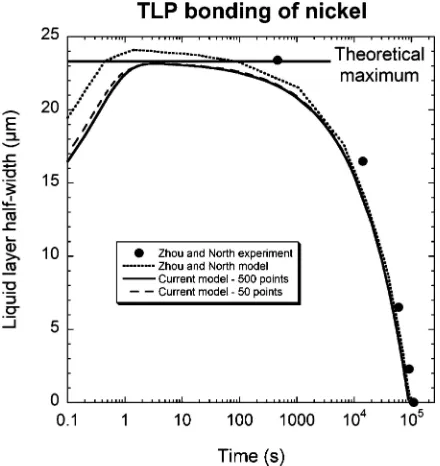
A variety of systems have been investigated, and re-sults agree well with experimental data. In Fig. 2, the half width of the liquid layer is plotted as a function of time for a Ni-P interlayer between pure Ni plates. Fol-lowing Zhou and North [2], a constant molar volume is assumed (irrespective of phase and composition)1_.

Ex-perimental data and model predictions from the same source are also presented in Fig. 2, for comparison with the present work.

The behaviour of the transient liquid phase predicted by both models is in accordance with our qualitative understanding of the process. The output is also in approximate quantitative agreement with experimen-tal data, even if very few discretisation points are used.

Both models assume that the number of atoms in any given volume does not vary with composition. Since phosphorous is an interstitial element in solid nickel, this assumption is not strictly correct. However, the

1_{This assumption will be made in all subsequent calculations.}

Figure 2 Predicted variation of liquid half-layer thickness with time as

Ni-P liquid solidifies between two sheets of pure Ni. Experimental data and numerical predictions of Zhou and North [2] are compared with output from the current model, using the same geometry and the same diffusion coefficient for phosphorus in solid or liquid nickel (1.8×10−7 or 5×10−6_cm2_s−1_{respectively). The ‘theoretical maximum liquid layer} thickness’ is calculated by neglecting fluid flow and diffusion in the solid and assuming a constant molar volume.

very low solidus concentration at the bonding temper-ature (0.17 at% P) means that errors arising due to this simplification are probably not significant. Assuming a constant molar volume permits the theoretical maxi-mum liquid layer thickness to be calculated—the thick-ness at which liquid is diluted to the equilibrium con-centration, without any diffusion of solute into the solid. For 12.5µm of Ni-19 at% P dissolving pure Ni until it reaches a concentration of 10.2 at% P (the liquidus concentration at the bonding temperature), the theoret-ical maximum liquid width is 23.2µm. The predictions of Zhou and North [2] exceed this value, indicating that their simulation does not conserve solute. The predic-tions of the present model do not exceed the theoretical maximum, which is consistent with the fact that it does conserve solute.

One experimental datum is also greater than the ‘the-oretical maximum’. This may be because the assump-tion of constant molar volume in the liquid is incorrect. Alternatively, liquid flow during experiments may have affected the thickness of the liquid layer as well as dif-fusion.

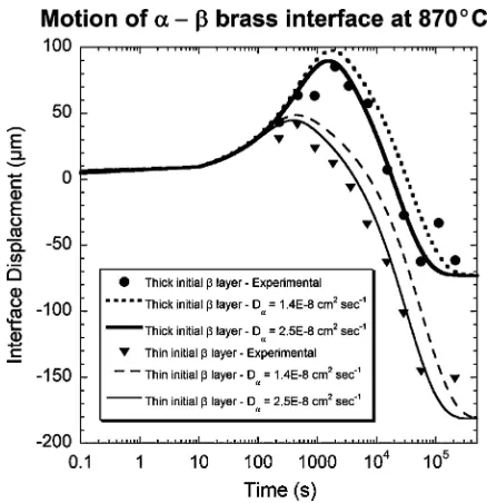
Figure 3 Experimental data and model predictions for the growth and

subsequent shrinkage of β-brass in contact with α-brass at 870◦C. Experimental data are from Heckel et al. [18], who used a constant thickness ofα-brass (749µm) and two different thicknesses ofβ-brass (381µm and 762µm) to investigate the motion of a phase boundary in this system. For each initial geometry, two corresponding predictions are plotted—the value of the diffusion coefficient of Zn inα-brass is unclear (see text).

in Fig. 3 for two different initial thicknesses ofβbrass (381 and 762µm).

There is some disagreement in the literature regard-ing the frequency factors ( A) and activation energies (Q) for the diffusion of zinc in Zn-rich α brass at 870◦C. Simulations were completed using two different diffusion coefficients, calculated using the published reference values [19]: either A = 0.016 cm2 s−1and Q = 124.5 kJ mol−1; or A = 1.7 cm2 s−1 and Q = 172.9 kJ mol−1_{. At a temperature of 870}◦_C,

these values correspond to diffusion coefficients D_α = 1.4×10−8_cm2_s−1_{and D}

α =2.5×10−8cm2s−1. In

theβphase, the diffusion coefficient was calculated to be 1.4×10−6_cm2_s−1_{using the undisputed reference}

values for A and Q.

The simulations using either value of D_α qualita-tively match the data, and there is close quantitative agreement with the second set of calculations. The differences between the model predictions indicate that user-specified diffusion coefficients have a significant effect on output, as expected. Clearly, correct diffusion coefficients are required for accurate predictions. The use of concentration-dependent diffusion coefficients might also improve the accuracy of the model. How-ever, on account of the paucity of data corresponding to the concentration-dependency of diffusion coefficients in most systems, such an extension has not been attempted.

4. Conclusions

A model has been developed to describe isothermal phase changes that are controlled by the diffusion of matter under the assumptions that

(1) There is local equilibrium at the interface; (2) Diffusion can be described by Fick’s second law; (3) The molar volume in each phase is constant.

The implementation considered in the present work models a two-phase diffusion couple in one dimen-sion (describing a planar geometry). Only binary sys-tems have been considered in the present work, and the diffusion coefficient in each phase is assumed to be independent of composition. None of these con-ditions are requirements of the method: extensions to cover many phases in higher dimensions, or sev-eral components and variable diffusion coefficients are possible.

The numerical scheme requires a system of coupled non-linear equations to be solved. The implementa-tion described above is fully implicit and decouples the problem into a set of linear equations which are solved iteratively. Calculations have been found to converge to accurate solutions, even with large timesteps. Large spacesteps can also be used with this method, as can non-uniform meshes.

Validation of the model has been possible using ex-perimental data from various systems, including TLP and solid-state diffusion couples. Agreement between model and observation is good, even for relatively large steps in space and time. In contrast with previous mod-els of diffusion-controlled phase changes, the scheme also conserves solute. It has first order accuracy in space and time.

The model has been implemented in the C program-ming language; optimising the efficiency of the code means that calculations can be completed very rapidly. The code is freely available to download from the Ma-terials Algorithm Project web-site: http://www.msm. cam.ac.uk/MAP

References

1.W. M A C D O N A L DandT. W. E A G A R, Ann. Rev. Mat. Sci. 22 (1992) 23.

2.Y.Z H O UandT. H.N O R T H, Modelling Simul. Mater. Sci. Eng.

1(4) (1993) 505.

3. J. Crank, Free and Moving Boundary Problems (Clarendon Press, Oxford, 1984).

4.Y. Z H O U, J. Mat. Sci. Let., 20(9) (2001) 841.

5.S. L I U, D. L. O L S O N, G. P. M A R T I N and G. R. E D W A R D S, Welding J. 70(8) (1991) S207.

6. R. M. Furzeland, J. Inst. Maths Appl. 26 (1980) 411.

7.Y. Z H O U, W. F. G A L E andT. H. N O R T H, Int. Mat. Rev.

40 (1995) 181.

8.H.N A K A G A W A, C.H.L E EandT.H.N O R T H, Met. Trans.

A 22(2) (1991) 543.

9.S. R. C A I N, J. R. W I L C O X andR. V E N K A T R A M A N,

Acta Mat. 45(2) (1997) 701.

10.T. S H I N M U R A, K. O H S A S AandT. N A R I T A, Mat. Trans.

JIM 42(2) (2001) 292.

11.C. W. S I N C L A I R, G. R. P U R D Y andJ. E. M O R R A L,

Met. Mat. Trans. A 31(4) (2000) 1187.

12.C. E. C A M P B E L LandW. J. B O E T T I N G E R, ibid. 31(11) (2000) 2835.

13.R. A. T A N Z I L L I andR. W. H E C K E L, Trans A.I.M.E. 242 (1968) 2312.

14.M. K A J I H A R AandM.K I K U C H I, Acta Met. Mat., 41(7) (1993) 2045.

Series in Computational Mathematics, Springer-Verlag, Berlin, 2003).

16. A. A. S A M A R S K I I andP. N. V A B I S H E V I C H, “Compu-tational heat transfer. V.1. Mathematical Modelling” (Chichester, Wiley, 1995).

17. J. C. T A N N E H I L L, D. A. A N D E R S O N and R. H. P L E T C H E R, “Computational Fluid Mechanics and Heat Trans-fer,” 2nd ed. (Taylor & Francis, London, 1997).

18. R. W. H E C K E L, A. J. H I C K L, R. J. Z A E H R I N G and

R. A. T A N Z I L L I, Met. Trans. 3 (1972) 2565.

19. C. J. S M I T H E L L, “Smithell’s Metals Reference Book,” 7th ed. (Butterworth, London, 1993).