Comparison of observations and modelling of surface mass balance variations in East Antarctica

Comparison of observations and modelling of

surface mass balance variations in East Antarctica

Author:

Bianca Kallenberg

A thesis submitted for the degree of Doctor of Philosophy of the Australian National University

June 2016

I hereby declare that the material contained in my thesis is entirely my own work, except of where accurate acknowledgement of another source has been made

Acknowledgements

My greatest gratitude goes to my supervisor Paul Tregoning for providing me with

the opportunity to conduct my research project, his guidance and encouragement

throughout my studies and for giving me the once in a lifetime opportunity to

travel to Antarctica for a closely related research project.

I would like to express my great appreciation to Anthony Purcell for his never

ending patience and guidance in teaching programming skills and setting up my

code. My sincerer gratitude goes to Rhys Hawkins for all his help and support in

solving remaining and newly occurring issues within my codes, for always being

around to answer questions and his effort to help solving issues, and to put me back

on track during my last months.

I wish to acknowledge Stefan Ligtenberg for his forthcoming support in explaining

his model, for providing me with the RACMO data set and his model results, and

his general help in establishing my program.

I would like to thank Achraf Koulali, Sebastien Allgeyer, Evan Gowan, Janosch

Hoffman and Christopher Watson for their advice, guidance and help on any

question I threw on them, programming issues and Antarctic research.

A special thank goes to Lydie Lescarmontier, not only for her support and advice in

glaciology but for her great company and supervision during our stay in Antarctica,

her friendship, support and her lovely cooking during the last month of my PhD.

I would like to thank my parents for their love and support, and for always

believing into me. I would like to thank my friends in Germany for good times

whenever I visit and of course all my friends here at RSES who made these past

years an unforgettable time. This includes my friends at the paddocks and my

incredible sweet horses Betsy and Shackleton, who always cheer me up regardless

of how I feel, and who give me so many amazing moments.

Last but not least all my love and thankfulness goes to my partner Kris Currie for

his never-ending patience, his support and for being my rock, walking with me all

Abstract

Mass balance changes of the Antarctic ice sheet are of significant interest due to its sensitivity to climatic changes and the contribution to changes in global sea level that is makes. In recent years, the Antarctic ice sheet has experienced increased temperatures inducing surface melting, accelerated ice flow and ice discharge but also an increase in accumulation. Geodetic

observations suggest variable behaviour across the ice sheet, with an increase in mass over a vast area of East Antarctica and substantial thinning in West Antarctica.

Despite considerable improvement on surface mass balance estimates using a variety of techniques, disparity remains mainly due to uncertainties of each

method and the unknown contribution of glacial isostatic adjustment, the response of the lithosphere to prolonged surface loads. Estimates of bedrock uplift rates are limited and existing models are poorly constrained due to the lack of observations as a result of the extensive permanent ice coverage in Antarctica.

This study investigates the possibility of combining and comparing altimetry and gravity observations by employing a regional climate model to simulate near surface climate and firn compaction, to separate the contributing ice sheet mass balance components of surface mass, firn compaction, ice

dynamics and glacial isostatic adjustment within the observed signals. The region of interest covers an area including Enderby, Kemp and Mac.Robertson Land, in East Antarctica, an area where an increase in ice mass and ice height has been recorded over the past decade. Despite the general agreement that the positive signal is primarily related to increased

snowfall, large uncertainties remain in bedrock uplift rates in this region due to the lack of observations.

Estimates of ice dynamic rates are obtained by removing modelled surface elevation variations, due to surface mass and firn compaction, from altimetry observations, which are subsequently employed in models of mass variations

Table of Contents

Chapter 1 - Introduction ... 1

1.1 Antarctic Ice Sheet ... 3

1.2 Ice sheet mass balance ... 9

1.3 Firn... 11

1.4 Glacial isostatic adjustment... 14

1.5 Antarctic Ice Sheet mass balance estimates ... 21

Chapter 2 - Satellite missions... 25

2 Introduction... 25

2.1 GRACE - The Gravity Recovery And Climate Experiment .. 26

2.1.1. Mission overview... 26

2.1.2. Gravity field solutions and errors ... 27

2.1.3 Relating gravity to surface mass... 30

2.2 Satellite Altimetry ... 33

2.2.1 Altimetry analysis techniques... 37

2.2.2 Converting elevation changes to volume and mass changes ... 41

2.3 GPS – Global Positioning System ... 43

2.4. RACMO2.1/ANT – Regional Atmospheric Climate Model 2.1 / Antarctica ... 44

Chapter 3 - Modelling of firn compaction and model sensitivity to climate variations ... 45

3 Introduction ... 45

3.1 Firn densification models ... 47

3.2.1 Firn compaction model... 53

3.3 Results... 56

3.4 Conclusion ... 76

Chapter 4 - Comparison of modelled and observed ice height and ice mass anomalies in Enderby Land, East Antarctica, and implications for ice dynamic rates ... 79

4 Introduction ... 79

4.2 Study site ... 82

4.3 Method... 84

4.3.1 Estimating Vice from ICESat measurements ... 86

4.3.2 Converting Vice into mass equivalent ... 87

4.3.3 Estimating Vice from GRACE measurements ... 88

4.3.4 Comparing ICESat and GRACE trends ... 89

4.3.5 Uncertainties ... 90

4.4 Results... 92

4.4.1 GRACE observations in Enderby Land... 92

4.4.2 Correcting GRACE observations for GIA ... 94

4.4.3 Estimating Vice from GRACE measurements ... 97

4.4.4 Surface elevation changes and estimating Vice from ICESat... 103

4.4.5 Comparison of estimated ice dynamic rates obtained from ICESat and GRACE observations... 112

4.5 Discussion ... 123

4.6 Conclusions ... 127

5 Conlcusions... 130

Chapter 1

Introduction

Understanding and estimating surface mass balance of the Antarctic Ice Sheet is of great interest, as the melting of the ice sheet contributes

significantly to global sea level changes. With a volume of ice of ~27 million km3 _{the Antarctic Ice Sheet (AIS) contains ~88% of all terrestrial ice} [Fretwell et al., 2013] and is the largest ice sheet on Earth. The remaining ice can be found in the Greenland Ice Sheet (~11%) and within smaller ice fields (~1%) such as permafrost and glaciers in the Himalayas, Patagonia, and Alaska [Solomon, 2007; Allison, et al., 2009].

The amount of freshwater held within the AIS is equivalent to 58.3 m of global sea level rise, with a potential contribution of 53.3 m from the East Antarctic Ice Sheet and 4.3 m from the West Antarctic Ice Sheet [Fretwell et al., 2013]. In comparison, the entire Greenland Ice Sheet contains an equivalent of 7.4 m of global sea level rise [Bamber et al., 2013]. Despite the

fact that global sea level has varied in the past, it had not changed significantly for several thousand years until the late 19th _{century [Church et} al., 2011]. Church & White [2011] found a rate of sea level rise of 1.7 ± 0.2 mm/year from 1900 to 2009, with an increase of 2.1 ± 0.2 mm/year between 1972 and 2008 alone [Church et al., 2011]. The rate at which global sea level

is increasing appears to be accelerating, especially since the late 20th _century [Church and White, 2011; Watson et al., 2015]. This correlates well with the beginning of rising global temperatures and, with global temperatures continuing to rise and major cities situated along coastlines, this will remain a serious concern in the future [Church et al., 2011]. Therefore, it is of great

To determine the contribution of the Antarctic Ice Sheet to future sea level changes a sound understanding about the processes within and beneath the ice sheet is required. However, due to the remoteness of the continent, persistent ice coverage and rough climatic conditions, obtaining observations and in-situ measurements is challenging and vast areas remain unsampled. Despite advances in observational technology and the employment of satellites to measure ice thickness, ice velocity, gravity and bedrock movement, large uncertainties remain in interpreting the signal and assessing the origin of the observed change. Satellites detect a general change in mass or height that can be derived from different causes. A change in mass that is observed by the Gravity Recovery And Climate Experiment (GRACE) mission can be induced by a change in surface mass or the distribution of mass within the Earth, primarily due to the viscoelastic response of the Earth’s lithosphere due to glacial isostatic adjustment [Shepherd et al., 2012]. Satellite altimetry observations are additionally affected by surface height changes due to the compaction of snow, in addition to variations in ice mass and glacial isostatic adjustment. Even though models exist for ice sheet elevation and thickness [e.g. Monaghan and Bromwich, 2008], ice flow velocities [e.g. Rignot et al., 2008], bedrock elevation [e.g. Fretwell et al., 2013], glacial isostatic adjustment [e.g. Whitehouse et al., 2012; Ivins et al., 2013 Peltier et al., 2015] or regional climate models to simulate the Antarctic near-surface climate [e.g. Bromwich et al., 2011; Lenaerts et al., 2012], large uncertainties remain within the models due to the lack of observations across the AIS. This leads to uncertainties in accurately interpreting satellite observations, as the signals have to be assigned and allocated to the correct origin and observed changes need to be distinguished and separated to obtain the amount of change within the contributing cause.

To contribute to the understanding of Antarctic surface mass balance changes and the interpretation of satellite observations I have compared modelled surface mass balance and surface elevation changes with observations from GRACE and ICESat, respectively, with the motivation to contribute to the estimation of surface mass balance variations of polar ice sheets.

when studying ice mass balance, followed by an introduction about the satellite missions and the regional climate model deployed in my research. To be able to correctly interpret altimetry measurements it is important to incorporate topographic changes due to the compaction of snow that occur within the firn layer that covers the AIS. Therefore, I developed my own firn compaction model that can be applied to my simulations on temporal elevation changes and I investigated the sensitivity of the model to small variations in the input values. This part of my research is covered in the third chapter

Finally I compared my modelled elevation changes in the firn layer with measurements from the ICESat mission to obtain an estimate of ice discharge values. Using my obtained estimates for ice discharge I then model temporal changes in mass and elevation to compare my modelled mass and height anomalies with observations from GRACE and ICESat. My method and results are described in the fourth chapter.

The thesis is completed with a concluding summary of my research in chapter five.

1.1 Antarctic Ice Sheet

the ice sheet a ~100 m thick firn layer is found, consisting of snow that has not melted and is slowly transformed to glacier ice through the process of densification [Ligtenberg, 2014]. Geographically, the continent is divided into the Antarctic Peninsula, West Antarctica and East Antarctica, separated by the Transantarctic Mountains (Figure 1.1). While the East Antarctic Ice Sheet (EAIS) is located on bedrock that is largely above sea level [Riffenburgh, 2006; Allison et al., 2009] the West Antarctic Ice Sheet (WAIS) is grounded on bedrock that is primarily below sea level, in places by more than 2000 m [Dalziel and Lawver, 2001; Allison et al., 2009; Fretwell et al., 2013]. Two large ice shelves are located between East and West Antarctica, the Ross Ice Shelf and the Filchner-Ronne Ice Shelf, each of an approximate size of 500,000 km2 _{[Rignot et al., 2013], while several smaller} ice shelves stretch along the coast.

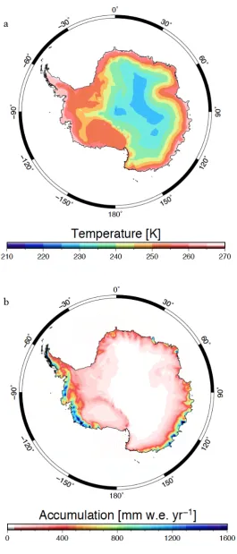
The climate of the AIS is strongly influenced by the surrounding Southern Ocean, the isolated location and size of the continent, and the terrain of the ice sheet. The average annual temperature across the ice sheet varies from approximately -60 degrees Celsius on the East Antarctic plateau to approximately -10 degrees Celsius near the ice sheet margins (Figure 1.2a). Although the major part of the AIS encounters sub-zero temperatures throughout the year, temperatures in coastal regions and on the Antarctic Peninsula can rise above zero degrees Celsius during warmer summer months. Due to such low temperatures, not much moisture is collected in the air above the ice sheet, creating a cold and dry climate. The highest snowfall rates can be observed at the Antarctic Peninsula and along the ice sheet margins, where more water vapour is collected in the air due to the surrounding ocean, while the interior does not receive much more snowfall than ~10 cm annually (Figure 1.2b), more often experiencing precipitation in form of diamond dust (ice crystals) [Schlosser et al., 2010].

is renowned to be closely related to changes in the SAM. Bromwich and Wang [2008] found that a high seasonal variability in MSLP in austral summer was consistent with a strong negative trend in the SAM. ENSO is the global-scale ocean-air interaction in the tropical western pacific (El Niño and La Niña) and a strong influence of ENSO on the Antarctic climate has been found [Sasgen et al., 2010; Fogt et al., 2010]. Transported by Rossby waves from the tropics towards the pole, it causes anomalies in the surrounding pressure system and changes in synoptic weather along the coast, primarily near the coast of West Antarctica [Monaghan and Bromwich, 2008; Sasgen et al., 2010; Boening et al., 2012]. Due to the ACT and cyclones, fierce storms regularly strike the continent, bringing warm moist air and precipitation towards the pole [Monaghan and Bromwich, 2008] and occasionally high precipitation events that occur only a few times per year but can bring up to 50% of the total annual accumulation [Schlosser et al., 2010]. Furthermore, the amount of water vapour in the atmosphere is additionally affected by the extent of sea ice, which varies from 4 million km2 _{in summer to 19 million km}2 _{in winter, having a significant impact on} seasonal atmosphere-ocean exchanges [Tietäväinen et al., 2008].

Figure 1.2a-b: Spatial distribution of the (a) average annual temperature and (b) accumulation, as provided by the regional climate model RACMO2/ANT.

a

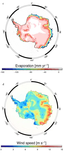
Figure 1.2c-d: Spatial distribution of (c) all sublimation and deposition processes combined (evaporation), positive is mass loss, negative is mass gain, and (d) average annual wind speed at 10 m above the surface, as provided by RACMO2/ANT.

c

The maximum snow transport occurs during autumn and winter [Parish and Bromwich, 2006] and is usually transported into the atmosphere [Scarchilli et al., 2010]. Drifting snow interacts with the atmosphere by increasing the lower atmosphere moisture content, thus leading to increased snowfall in regions where the atmosphere usually contains little moisture [Lenaerts and van den Broeke, 2012]. Locally, drifting snow erosion and deposition have a significant impact on snow mass variations and need to be included in surface mass balance estimates (Figure 1.2d) [Lenaerts and van den Broeke, 2012].

1.2 Ice sheet mass balance

2014]. In Antarctica, zones of exposed blue ice are formed in regions where ablation exceeds accumulation and ~1 % of the EAIS is covered by wind-induced (e.g. Byrd Glacier) and melt-wind-induced (e.g. Lambert Glacier and Amery Ice Shelf) blue ice areas [van den Broeke et al., 2006; Ligtenberg et al., 2014].

Ablation processes include the discharge of snow and ice due to ice melting, both at the surface and at the glacier base, and erosion and sublimation (the direct transition from solid to gas without entering the liquid phase) on the surface. In a cold environment like Antarctica, sublimation is the dominant ablation mechanism, favoured by dry air and strong winds [Cuffey and Paterson, 2010]. While sublimation occurs year-round in some parts of Antarctica (e.g. Dry Valleys [Fountain et al., 2006]), in other regions short ablation periods during summer are usually interrupted by returning cooling events and/or snowfall. Melt streams form in regions where temperatures occasionally reach the melting point. However, not all of the meltwater drains, but refreezes, either on the surface, percolated within a cold snow or firn layer, or within fractures and crevasses [Cuffey and Paterson, 2010]. The primary mechanism of mass output of the AIS is by ice discharge into the surrounding ocean as the ice sheet passes the grounding line (boundary between grounded and floating ice) and forms floating ice shelves. This leads to iceberg calving and basal melting at the bottom of the floating ice shelves [Zwally et al., 2002; Cuffey and Paterson, 2010]. The rate at which these processes contribute to the mass balance of the entire ice sheet over a period of time, determine the change of total mass.

To emphasise the contribution of the accumulation and ablation processes, surface mass balance (SMB) can be written as:

SMB = A – S – WE + WD – MRu,

Where A represents accumulation, S sublimation, WE and WD wind erosion and wind deposition of surface snow, respectively, and MRu meltwater runoff. All terms represent a change in mass and are given in kg m-2 _yr-1_{. The} distribution of snow by wind is negative where it erodes and positive where

snow erosion can be neglected on a continental scale but is found to significantly affect local SMB changes [Lenaerts and van den Broeke, 2012]. Sublimation can also be either positive or negative as sublimation usually exceeds depositions due to water vapour [Cuffey and Paterson, 2010]. Although the process of meltwater runoff is small in Antarctica since most of the meltwater refreezes locally, it cannot be neglected, as meltwater runoff occasionally occurs in some parts of the AIS. To obtain the overall change in mass balance (MB) the volume of ice discharge (D) over the grounding line has to be subtracted from the surface mass balance:

MB = SMB – D.

1.3 Firn

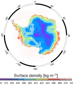
Firn is the material that composes the intermediate product between snow and ice. Usually the term “snow” is restricted to the material that has not changed since it fell and still has its initial density [Cuffey and Paterson, 2010]. In Antarctica the density of fresh snow is typically ~350 kg m-3_{, but} can vary between 300 kg m-3 _{in the cold interior and up to 450 kg m}-3 _along the coastline [Helsen et al., 2008b; Ligtenberg et al., 2011]. Due to cold temperatures and nonexistent regular snowmelt events in Antarctica, surface snow is constantly buried during precipitation events, constantly increasing surface loads. Once fresh snow is deposited, different stages of densification are passed before it reaches the state of dense glacier ice. The densification process is highly dependent on accumulation rate and temperature and is commonly referred to as “firn compaction” [Cuffey and Paterson, 2010; Arthern et al., 2010; Ligtenberg et al., 2011]. During the compaction, air is removed and snow crystals are compressed, deformed and repositioned. As a result, the density changes with depth, overburden pressure and temperature, and increases until the density of ice (approximately 917 kg m-3₎ is reached [Herron and Langway, 1980; Cuffey and Paterson, 2010]. Through this process the firn layer compacts, reducing its thickness and thus the

elevation of the ice sheet. This is an important factor when measuring ice surface heights, as the thickness of the firn layer constantly changes, and surface elevation changes may be due to the densification of the firn layer rather than mass loss [e.g. Li and Zwally, 2004; Riva et al., 2009; Li and Zwally, 2010].

Within the transformation process, Herron and Langway [1980] identified three stages of densification with the fastest densification rate in the first stage; here the dominant mechanism is packing, settling and re-arranging of snow grains. After reaching a density of about 550 kg m-3 _{densification slows} down significantly and compaction occurs mainly due to material transfer by sublimation, diffusion and deformation processes. This stage continues until the pore close-off depth is reached and air bubbles are trapped within the ice, usually at a density of approximately 830 kg m-3_{. In the last stage,} remaining air bubbles undergo further compression until the density of glacier ice,~917 kg m-3_{, is reached [Herron and Langway, 1980; Ligtenberg et} al., 2011]. In regions where surface temperatures occasionally climb above freezing, meltwater will occur and can penetrate into the firn layer. During such events, water percolates down through the firn layer, filling up the air pores and will partly remain attached to snow crystals. Once the meltwater reaches a layer with temperatures below zero it will refreeze, replace available air space with ice and efficiently compact this layer [Ligtenberg, 2014].

situation is often assumed in order to estimate the firn compaction, with the attempt to establish time-dependent models [e.g. Zwally and Li, 2002; Reeh, 2008; Li and Zwally, 2011; Ligtenberg et al., 2011]. A detailed description of firn densification models of the AIS can be found in Chapter 3.

1.4 Glacial isostatic adjustment

There are several possibilities for observing and estimating Glacial Isostatic Adjustment (GIA) rates. Fennoscandia is described as the key area for GIA research due to its long settlement history with an early start of scientific investigations that commenced in the late 17th _{century [Steffen and Wu,} 2011]. To study present-day GIA rates, observations of relative sea level, tide-gauges, shoreline tilting, geomorphology, as well as GPS and gravity measurements are used, to provide information about crustal movements [e.g. Whitehouse et al., 2012a,b; Peltier et al., 2015]. To cover a time period that can be dated back to several thousand years it is necessary to look at relative sea level (RSL) observations that indicate a rise or fall in any particular coastal area since the LGM. The magnitude of RSL movement is governed by changes in ocean water volume, isostasy in reaction to mass redistribution, and tectonic uplift or subsidence of the Earth’s crust, and varies with distance from the former ice sheet. Surface-pressure is greatest in the centre of an ice sheet, hence, the isostatic component is largest in that area and gradually decreases towards the former ice edges, being negative outside the ice sheet and over the oceans and small but positive for far-field continents [e.g. Johnston and Lambeck, 1999].

history of the Late Pleistocene Antarctic and Arctic ice sheet [e.g. Nakada and Lambeck, 1988; Nakada et al., 2000] as well as the Laurentide and Fennoscandia ice sheets [e.g. Peltier, 2002; Peltier, 2004], respectively, and are supported by additional observations in and near Antarctica where available [e.g. Whitehouse et al., 2012a; Ivins et al., 2013; Argus et al., 2014]. The timing of melting events and the contribution of individual ice sheets to sea level needs to be estimated to allocate ice sheet melting history and relative sea level observations. Therefore, ice sheets that covered the continents during the Late Pleistocene and Holocene have to be reconstructed in their extent and thickness. The prediction of uplift rates in GIA models strongly depends on the ice history used and the underlying Earth rheology model. While there is general agreement amongst scientists that the Antarctic ice cover during the LGM was more extensive than it is at present, it is not agreed to what extent [Ivins and James, 2005]. Nakada and Lambeck [1988, 1989] established three Arctic and four Antarctic models, respectively, to construct a correlation between modelled and observed sea-level changes, each model differs in ice volume, timing of melting and its contribution to sea-level. More recently, Nakada et al. [2000] updated the models by comparing field observations and modelling results, constraining a maximum (ANT5) and minimum (ANT6) ice-loading history model of the AIS.

measurements of vertical bedrock motion [Argus et al., 2014]. To enhance the ICE-6G_C for Antarctica, observations of vertical and horizontal crustal movement of 59 GPS sites in Antarctica were used and the ice thickness is adjusted to enable the model to fit GPS uplift rates, ice thickness change data and sea level histories. The model is found to fit the totality of these data well [Argus et al., 2014].

In 2005 Ivins and James [2005] developed the IJ05 model to provide a GIA model for Antarctica. Their model is based on radiocarbon dating, marine records, sedimentary core data, as well as moraine and lacustrine data of ice-free exposures, and both bathymetric and seismic mapping, respectively. Compared to the ICE-5G model, the IJ05 predicts a substantially smaller meltwater input into the oceans (65% less volume than the ICE-5G model), assuming that more meltwater had been contributed from other ice sheets. Furthermore, they used a different forward model to predict vertical crustal velocities, strongly depending on mantle creep strength or mantle viscosity [Ivins and James, 2005]. Ivins and James [2013] have improved their IJ05 model to develop IJ05_R2 by incorporating new datasets that have become available: a substantially improved set of geological and ice core data, and GPS vertical motion observations.

Prior to this, Whitehouse et al. [2012a,b] developed a new deglaciation model and GIA model for Antarctica, likewise building upon the work of Ivins and James [2005]. Beside the widely available datasets of marine and terrestrial geological and geophysical observations, and recently introduced past ice sheet extent studies from multibeam (swath) bathymetry, they have synthesised the existing data and combined them with a numerical ice-sheet model to reconstruct the AIS at different time steps [Whitehouse et al., 2012a]. The result of their approach is a new deglaciation model, W12, (and W12a, an adjusted version of the initial model to fit GPS observations across the Antarctic Peninsula) that presents an estimate for the ice sheet volume at the LGM being lower than previous studies and an improved GIA model that fits relative sea level data and GPS observations. The outcomes of the improved deglaciation models (W12 and IJ05_R2) result in a smaller GIA correction, directly affecting ice sheet mass balance estimates by a difference of ~70 Gt/yr (shown in Table 1.2) [Velicogna and Wahr, 2013].

uplift rates and ice mass balance changes derived from satellite observations. Riva et al. [2009] published a present-day GIA model derived from using a hybrid ice-firn surface density model to estimate mass changes from altimetry, and combined these observations with GRACE observations of mass change (Chapter 2, Section 2.1) to separate GIA from surface processes. Under the assumption of a bottom (rock) and a top (ice/firn) layer of different densities and thickness, they modelled GIA uplift rates as:

HGIA = (MGRACE – !surf) HICESat / (!rock - !surf)

where HGIA describes the variation in bedrock topography, MGRACE and HICESat represent the mass change and elevation changes as observed by GRACE and ICESat (Chapter 2, Section 2.1 and 2.2), accordingly, and !rock and !surf the average density of the rock and surface layers, respectively [Riva et al., 2009; Gunter et al., 2014]. Their model results are in good agreement with the IJ05 model and glaciological models [e.g. Huybrecht, 2002] but differed significantly from the ICE-5G model [Riva et al., 2009].

Gunter et al. [2014] recently revisited the approach by Riva et al. [2009], by including a firn densification model and SMB estimates, with the aim to account for surface mass processes:

HGIA = MGRACE – [(HICESat - HFirn) !a+ MFirn] / (!rock - !a)

with HFirn and MFirn representing changes in height and mass due to firn compaction, and where the density !a varies between 917 kg m-3_{, when} (HICESat - HFirn) < 0 and | HICESat - HFirn| > 2 , and the density difference between ice/snow, when (HICESat - HFirn) > 0 and | HICESat - HFirn| > 2 . represents the uncertainty of the height estimates, which is derived from the firn compaction and the altimetry data set:

,

!h

!h

!h

!h = !ICESat 2 _+!

Firn 2

(1.3)

(1.4)

with the uncertainty in the ICESat observations, , and in the firn densification model, , respectively [Gunter et al., 2014]. The results for the GIA estimates show a general agreement with the IJ05 and W12a models, showing a slight subsidence in East Antarctica, and uplift in West Antarctica, namely between the Ross and Filchner Ronne Ice Shelf. Additionally, the overall estimate of ice mass changes are similar to results of Shepherd et al. [2012], King et al. [2012] and Sasgen et al. [2013].

In 2002, before the launch of the GRACE satellites, Velicogna and Wahr [2002] presented simulated results for a method to separate Antarctic GIA and ice mass balance using GRACE and altimetry data. By simulating GRACE and ICESat data they obtained a root-mean square accuracy of 5.3 mm yr-1 _{for GIA and 19.9 mm yr}-1 _{for MB. They mentioned that their largest} source of error within the combined signal is the effect of unknown mass of accumulation and firn density, which is why they added GPS measurements as additional constraints. Their technique was based on recovering spatial variability of ice mass trend and GIA signals to initially solve for SMB and GIA before adding GPS measurements of vertical velocities to solve for firn densities.

Using an analogous iterative approach as described by Wahr et al. [2000], ICESat data alone can be used to determine ice mass changes. These data are assumed to be only sensitive to ice thickness changes and have not been corrected for firn densification and GIA, as SMB estimates would be contaminated regardless, due to model uncertainties [Wahr et al., 2000; Velicogna and Wahr, 2002]. The MB estimate from ICESat is used to calculate the rate of change in the geoid and is removed from the GRACE data. The remaining change in the geoid from the GRACE data is interpreted as GIA signal, which is subsequently removed from the ICESat observations. That process is repeated to obtain a better SMB estimate [Wahr et al., 2000] until the improvement is negligible [Velicogna and Wahr, 2002]. According to Velicogna and Wahr [2002] using two observables to determine three unknowns is the limiting error in the SMB recovery. To overcome this issue they added GPS point measurements of vertical velocity by estimating GIA from the difference between GPS velocities and computed GIA estimates. This step is applied to the last iteration of the GRACE/ICESat

!ICESat

compaction trends, which subsequently can be used to correct the SMB estimations. In spite of their simulations being successful, their approach has not been presented with real data from actual GRACE and ICESat observations.

Table 1.1: Approximate present-day uplift rates for various locations across Antarctica in [mm yr-1_{] as modelled by the GIA models described in the text. The} data is taken from Figure 14 in Whitehouse et al. [2012], Figure 4 and 5 in Ivins and James [2013] and Figure 6 in Argus et al. [2014].

GIA model

South Pole

Mawson Dumont D’Urville

Edward VII Land

Palmer Land

General Belgrano

II

ICE-5G (Peltier)

3.7 3.3 0.5 5 7 2.4

IJ05_R2 (Ivins

and James)

0 1 1 2 2.5 1.5

W12a (Whiteho

use et al.)

0 1 1.4 4 0.5 0.5

ICE-6G (Peltier)

1.5 Antarctic Ice Sheet mass balance estimates

There are different techniques used to evaluate ice mass balance: measuring the change in mass, the change in volume, which is subsequently converted to a change in mass through firn density, and the mass budget method (MBM).

The gravimetric method is based on direct observations from the Gravity Recovery And Climate Experiment (GRACE) satellite mission, which monitors the Earth’s gravity field. Mass changes within the ice sheet directly affect spatial and temporal changes in the regional gravitational field and are therefore detected by GRACE. Besides changes in ice mass it is also necessary to correct for other possible mass variations, such as ocean tides and the deformation of the Earth’s crust as a response to prolonged ice loads (GIA). A more comprehensive description of the GRACE space mission, observations and the method to estimate ice sheet mass balance can be found in Chapter 2, Section 2.1.

The second method is based on using satellite altimetry to monitor temporal surface elevation changes of an ice sheet by measuring the distance between the ice surface and the satellite. A change in height can be related to a change in the volume of an ice sheet which, subsequently, can be converted into a change in ice mass if the density is known. However, surface elevation is also affected by the densification process of snow and glacial isostatic adjustment, therefore, models have to be applied to correct for both processes. This method, together with a comprehensive explanation about satellite altimetry missions and converting altimetry observations to mass changes, is described in more detail in Chapter 2, Section 2.2.

fill in the gaps. More commonly used are regional atmospheric climate models that simulate near surface climate patterns across the entire ice sheet [e.g. van de Berg, et al., 2006, Lenaerts et al., 2012]. The quantity of mass output is determined by the amount of ice that discharges across the grounding-line, which can be assessed by measuring the velocity of ice flow and the ice thickness at the grounding line [e.g. Rignot, 2002]. To obtain ice velocities, interferometric synthetic aperture radar (InSAR) satellite images are used, while the ice thickness can be estimated either by using ice penetrating radar or is derived from the location of the actual grounding line [Rignot et al., 2011; Ligtenberg, 2014]. The map of ice velocities across Antarctica has been updated by Rignot et al. [2008], presenting a nearly complete map from InSAR data collected between 1992-2006 using ERS-1/2, Radarsat-1 and Japanese Advanced Land Observation Satellites. Ice velocities are presented with a precision of 5-50 m yr-1 _{and short-time variations are} averaged out. The grounding line of the glaciers is mapped with a precision of 100 m all around Antarctica, derived from surface elevation under the assumption that ice is in hydrostatic equilibrium with seawater. The SMB is determined using RACMO2/ANT and averaged for the period 1980-2004 and is compared to ice flux for each glacier [Rignot et al., 2008]. In general, ice dynamics are not well known and it has been pointed out by Rignot et al. [2008] that mass budget is more complex than previously indicated and that changes in glacier dynamics may dominate ice sheet mass budget.

Another approach that has been applied to estimate present-day surface mass trends and GIA in polar regions is to combine GRACE observations with Ocean Bottom Pressure (OBP) and GPS measurements [Wu et al., 2010]. A simultaneous global inversion of derived linear trends from GRACE and OBP records, combined with surface velocities of globally distributed GPS sites is used to separate global surface mass and GIA in geodetic data. This is done by combining the geodetic data with a priori information on GIA dynamics and the spatial extent of deglaciation from glaciological and geological data [Wu et al., 2010].

Chapter 2

Satellite missions

2 Introduction

In recent years satellite missions have significantly contributed to and improved our understanding and knowledge of temporal and spatial variations of the Earth’s atmosphere and climate, the Earth’s gravity field and surface elevation. Satellites orbiting the Earth on repeat cycles help us to monitor changes that occur over time. Due to the limitation of conducting fieldwork in remote areas, scientific satellite observations in polar regions have increased our understanding on present-day ice mass variations across the polar ice sheets, providing new insights into climatic and atmospheric fluctuations near the poles, ice sheet mass balance, ice thickness and glacial isostatic adjustment.

The primary satellite missions to study changes of the polar ice sheets are the Gravity Recovery And Climate Experiment (GRACE) mission to measure variations within the Earth’s gravity field, and satellite altimetry (e.g. ENVISAT, ICESat, CryoSat-2) to obtain time-series of surface elevation changes. Additionally, GPS measurements are used to detect vertical bedrock movements of the lithosphere beneath the AIS to observe the elastic and viscoelastic response of the Earth’s crust.

adjustment. Altimetry observations are further sensitive to changes caused by the compaction of firn, as this leads to a reduction of the firn layer thickness that covers the ice sheet, and detected elevation changes need to be corrected for the compaction rate. This chapter focuses on the satellite missions that are used in this thesis to study present-day surface mass balance and bedrock uplift rates as monitored by the satellites. It furthermore provides a description of the regional climate model RACMO2.1, that is used to model mass and height anomalies, which are compared with gravity and altimetry observations from the GRACE and ICESat mission, respectively.

2.1 GRACE - The Gravity Recovery And Climate

Experiment

The Gravity Recovery And Climate Experiment (GRACE) space mission was launched in 2002 to monitor temporal mass variations in the Earth system. It is a joint mission by NASA and the German Aerospace Centre (DLR – Deutsches Zentrum fuer Luft und Raumfahrt) and was designed to operate for five years [Tapley et al., 2004]. Currently, GRACE operates in an extended mission phase, which will hopefully continue through to 2017 when the follow-up mission is planned to be launched. Due to the fact that, even 12 years later, the GRACE satellites still provide global maps of the Earth’s gravity field, the gravity experiment is one of the most successful space missions. However, battery life as well as fuel availability on GRACE A are now important issues and operation times are reduced during eclipse seasons to maximise the remaining lifetime [Kruizinga and Williams, 2015].

2.1.1. Mission overview

mapping the entire globe to measure minor variations in the Earth’s gravitational field [Tapley et al., 2004]. The spatial resolution at which GRACE can map the global gravity field is 400 km to 40,000 km [Tapley et al., 2004]. Measurements of mass anomalies are made by the gravitational influence on the satellites causing a change in the distance between the two satellites. A very sensitive K/Ka-band microwave ranging system measures these fluctuations in the along-track direction of the satellites [Tapley et al., 2004]. Additionally, onboard are highly accurate accelerometers that measure non-gravitational accelerations acting on the satellites, and GPS receivers for precise positioning and time tracking. By implementing an inversion of the GRACE observations, it is possible to derive temporal global solutions of the Earth’s gravitational field as monthly [e.g. Tapley et al., 2004; Ramillien et al., 2006] or 10-daily [Bruinsma et al., 2010] estimates. GRACE data are mainly utilised to study the redistribution of water in the Earth’s system, including ocean circulation [e.g. Wahr et al., 1998; Janji" et al., 2012], sea-level changes [e.g. Chambers and Schröter, 2011], ice-sheet mass balance [e.g. Velicogna and Wahr, 2006; Horwath et al., 2012], continental water exchanges and storage [e.g. Ramillien et al., 2005; Swenson and Wahr, 2009], droughts and flood [e.g. Freeport et al., 2013], as well as determining glacier and ice-sheet variations and to track solid Earth density variations and crustal movement [e.g. Velicogna, 2009; Wu et al., 2010; Purcell et al., 2011; Velicogna and Wahr, 2013].

2.1.2. Gravity field solutions and errors

the Information System & Data Center at the German Research Center (GFZ).

degree 80 (GRGS) and 96 (CSR) [Lemoine et al., 2013; Bouman et al., 2014]. The GRACE solutions used for this thesis are provided by the Groupe de Reserches de Géodésie Spatiale (GRGS)

Release 02

In 2009, GRGS published the second series (RL02) of gravity fields in form of 10-day gravity field models as described by Bruinsma et al. [2010]. The processing strategy employed normalised spherical harmonic coefficients up to degree and order 50 at a 10-day interval, with a spatial resolution of ~400 km. The new time-variable mean gravity field EIGEN-GRGS.RL02.mean-field was used as the reference model, the background models IERS2003, FES2004 and MOG2D were used to correct for various tidal variations, such as the gravitational potential of the Earth and that of external bodies [McCarthy and Petit, 2003], ocean tides that affect solid Earth and ocean pole tide deformations [Desai, 2002], and the global barotropic response to atmospheric forced variability of the oceans [Carrère and Lyard, 2003], respectively [Bruinsma et al., 2010]. The ECWMF climate model was used to model atmospheric effects. Due to a stabilisation process during their generation by constraining the coefficients (degree 2 to 50) to the coefficients of the static field, noise in form of North-South striping in the GRGS solutions is already reduced and subsequent filtering is not necessary for the analysis [Lemoine et al., 2007, Bruinsma et al., 2010].

Release 03

been undertaken and the maximum degree has been extended from 50 to 80, improving the spatial resolution [Lemoine et al., 2013]. Additionally, a new “mean field” has been computed and the inversion process is now based on a truncated single value decomposition scheme [Biancale, 2012]. However, due to an error at high latitudes in the FES2012 tidal model, the GRGS RL03 solutions cannot be used in polar areas between 82 and 90 degrees at present [Biancale, 2012].

I chose to use the GRGS solutions for my research due to their stabilisation process that is applied to reduce noise in the form of North-South striping by regularising the inversion for spherical harmonic coefficients. Bruinsma et al. [2010] stated that regularising geopotential coefficients leads to “more accurate geoid difference/EWH anomaly maps than a-posteriori filtering of solutions, because the level of stabilisation of a solution depends on the sensitivity of a given spherical harmonic coefficient to the normal equation system”. Generally both signal and noise are attenuated randomly when filtering and smoothing geopotential solutions, as the data distribution and quality is not known [Lemoine et al., 2007; Bruinsma et al., 2010]. Due to their stabilisation process, the GRGS solutions are also less prone to signal contamination (leakage), which is enhanced by increasing the radius of the Gaussian smoother [Bruinsma et al., 2010; Velicogna and Wahr, 2006].

2.1.3 Relating gravity to surface mass

The viscoelastic deformation is a long-term signal of GIA in regions that were ice covered during the last ice age [Wahr et al., 1998] whereas elastic deformation is an instantaneous effect caused by surface loads such as hydrological variations. All these gravitational changes affect the orbit of the twin satellites of the GRACE space mission [Tapley et al., 2004] and provide a measure to understand mass transport processes in the atmosphere, hydrosphere, cryosphere and geosphere.

The Earth’s gravity field describes the shape of a geoid, which is the equipotential surface that approximates global mean sea level, often described as a sum of spherical harmonics [Wahr et al., 1998]. Spherical harmonics are a common approach for modelling a gravitational field of a planetary body. With Equation (2.1) we can calculate the change in the geoid [Wahr et al., 1998]:

where R is the Earth’s radius, Pnm are the fully normalized Legendre functions, n and m are degree and order of the spherical harmonic coefficients, # and $ are colatitude and longitude, and %Cnm, %Snm are the dimensionless Stoke’s coefficients of the GRACE anomaly fields, respectively, at time t. While Equation (2.1) calculates the general change in the geoid as a function of position and time on Earth, the contribution of surface mass loads, expressed in water equivalent (w.e.), that would be necessary to cause that explicit change in the geoid can be derived [Wahr et al., 1998] using:

where kn are elastic Love loading numbers [e.g. Pagiatakis, 1990] and the elastic Stoke’s coefficients at time t, representing the elastic component of the GRACE signal. A vertical elastic deformation is caused by the deformation of the Earth’s crust as a quick response to surface load

U

(

)

n

!

(

)

(

( )

( )

)

N

!

Uw.e. !

,",t

(

)

m=0 n

!

(

)

2n+1 1+kn"

#Cnm elast

t

( )

t

( )

(

)

n=2 N

!

!Cnm elast,!

Snm elast

(2.1)

changes by losing or gaining weight and can be described with the elastic Love loading numbers hn and kn [Davis et al, 2004]:

The GIA associated long-term contribution of the viscoelastic deformation can be approximated by [Purcell et al., 2011]:

where represents the viscoelastic component of the GRACE signal, and hn and kn the viscoelastic Love loading numbers, depending on the degree [Purcell et al., 2011].

The GRACE anomalies are a combination of both components, elastic (induced by changes in surface mass loads) and viscoelastic (GIA) effects, and the total change in the geoid is the sum of the two effects [Tregoning et al., 2009]. Therefore, to allocate the observed mass changes to the correct geophysical sources it is necessary to separate the elastic and viscoelastic components [Wahr et al., 1998]. This is not straight forward, since there is only one GRACE observation but it is a sum of the effects of two processes.

Uelast

(

)

m=0

n

!

(

)

hn elast

1+kn

elast "Cnm elast

t

( )

elast

t

( )

(

)

n=2

N

!

Uvisco

(

)

m=0 n

!

(

)

hn visco

kn

visco "Cnm visco

t

( )

visco

t

( )

(

)

n=2 N

!

!Cnm visco,!

Snm visco

(2.3)

2.2 Satellite Altimetry

ERS-1, ERS-2 and ENVISAT 1991 - 2012:

The first of the European Remote Sensing satellite missions, ERS-1, was launched in 1991 and orbited the Earth on a repeated cycle of ~35 days to a latitude of about 82.4 degrees south. The footprint size of the radar altimeter was 1.7 km and the height accuracy was over 73 cm over ice sheets [Nguyen, 2006; Rémy et al., 2014]. The mission continued until 1996 when it was replaced by the follow on mission ERS-2, which continued until 2001. In 2002, ENVISAT was launched and collected surface topography observations until 2012 when, unexpectedly, contact was lost with the satellite. Both ERS-2 and ENVISAT had the same orbit and repeat cycle as ERS-1. Despite the same footprint size, height accuracy for the ENVISAT mission improved to ~35 cm compared to > 73 cm for the ERS-missions. All three missions were equipped with a Ku-Band radar altimeter and repeatedly orbited the Earth with a 98.5 inclination [Horwath et al., 2012]. Recently the REAPER (REprocessing of Altimeter Products for ERS) project has been finished, covering both ERS-1 and ERS-2 missions, providing a greatly improved dataset [Gilbert et al., 2014]. Studies using ERS data to study the AIS include work from Wingham et al. [1998], Zwally et al. [2002] and Zwally et al. [2005], studies using ENVISAT data include Horwath et al. [2012], Flament and Rémy [2012], Rémy et al. [2014], Michel et al., [2014]. The follow up mission SARAL/AltiKa was launched in February 2013, to measure the Earth’s topography on exactly the same orbit, extending the previous three missions [Rémy et al., 2014; Michel et al., 2014].

ICESat 2003 - 2009:

et al., 2005]. The satellite orbited the Earth at around 600 km altitude at an inclination of 94° with a modified ground track period of 91-days and provided latitudinal coverage up to 86 degrees. For a period of around 33 days the lasers were turned on up to three times a year [Schutz et al., 2005; Abshire et al., 2005] until Laser 2 failed in 2004 due to the same failure as Laser 1 [Abshire et al., 2005]. To mitigate the rapid energy decline that occurred in the first two lasers, Laser 3 was operated at a lower temperature [Abshire et al., 2005], resulting in a slower energy decline rate and thus successfully operated until 2009. Although the data quantity and spatial resolution was significantly reduced and tracks were rarely repeated precisely [Slobbe et al., 2008; Pritchard et al., 2009; Sørensen et al., 2011], the altimeter recorded ice height changes to an accuracy of < 1.5 cm yr-1 _averaged over 100 x 100 km sections [Nguyen, 2006; Hoffmann, 2014].

ICESat carried the Geoscience Laser Altimeter System (GLAS), consisting of a 1064 nm infrared laser pulse to measure dense cloud heights and surface topography [Zwally et al., 2002; Schutz et al., 2005]. The instrument had three identical laser transmitters, a receiver telescope, a solid-state detector, a subsystem to measure the angle of the laser pulses and waveform digitisers to record the laser backscatter signal [Zwally et al., 2002]. On-board GPS receivers allowed orbit determinations to better than 5 cm. Star-trackers, measuring the position of stars, enabled pointing accuracy to locate footprints to 6 m horizontally and the spacecraft attitude controlled the laser beam to within 35 m of reference surface tracks [Zwally et al., 2002].

CryoSat-2 2010 - present:

which consists of an antenna subsystem, radio-frequency unit and digital processing unit. There are three different measurement modes available to choose the antenna on reception, transmitted bandwidth and timing of transmitted chirps [Wingham et al., 2006]. The low-resolution mode (LRM) is used to measure the topography of the oceans and the smooth interior of ice sheets. For improved sampling along steep ice sheet margins the higher pulse repetition frequency of the synthetic aperture mode (SARM) and synthetic aperture interferometric mode (SARInM) is used [Wingham et al., 2006].

In addition, ocean-loading and ice shelf tidal corrections are applied to the altimetry signal, as well as atmospheric delay corrections for laser altimeters [Zwally et al., 2002]. When using laser altimeter correcting for atmospheric forward scattering and delay is important as the performance of the pulse signal can be degraded when in contact with cloud cover. When the cloud cover is extremely thick the pulse reflects of the clouds, not measuring the Earth’s surface but the height of the cloud cover instead [Fricker et al., 2005].

2.2.1 Altimetry analysis techniques

Different techniques are used to analyse altimetry observations, which can be broadly broken into two categories: crossover and along-track analysis. Each method has advantages and disadvantages. A satellite that orbits the Earth covering both polar regions has an ascending (travelling south to north) and descending (travelling north to south) track. The location where both tracks intersect is called the campaign crossover [e.g. Brenner et al., 2007]. The ground track of the satellite shifts due to perturbations of the orbit, which results in varying deviations of the repeated ground track. Therefore, the surface topography needs to be determined to correct elevation changes due to surface slope rather than to changes in ice mass. Alternatively, the topography can be estimated in the same least squares inversion used to determine observed ice height changes [Flament and Rémy, 2012].

repeatedly done for all sequences, which are subsequently combined into one elevation time series [Zwally et al., 2005]. Brenner et al. [2007] introduced a polynomial fit to calculate the intersection of the ascending and descending ICESat ground track, and estimated the elevation at the crossover by interpolating available heights along the ground track closest to the crossover location. Gunter et al. [2009] used cubic spline interpolation on ICESat crossover data points within ~400 m to refine the position of the campaign crossover. A cluster of inter-campaign crossovers, using ground tracks from different laser campaigns (using the ground track of a different laser), is used to determine the height at the crossover using cubic-spine interpolation. Although the crossover analysis technique is very effective on ICESat tracks at high latitudes, it becomes less accurate towards the coastal areas of the Antarctic ice sheet, as the density of crossovers is highest near the poles and decreases from ~ 11,340 near 85.5° south to ~ 70 near 70.5° south, over an average 100 x 100 km2 _{area, due to the chosen orbit of the satellite [Nguyen,} 2006]. However, this method is based on the assumption that the signal of height changes is constant, which may be true in the dry interior of Antarctica but not near the coastal margins, where strong slopes impede estimations of the rate of change.

method that is based on elevation differences at crossover points and can be written as the sum of a signal, a terrain slope contribution and a noise term, which is assumed to be random. They used only overlapping footprints of the ICESat mission to eliminate the need for terrain smoothing and interpolation, which is only needed to correct the obtained elevation differences for the influence of slope. However, the centre points of the overlapping footprints generally do not overlap and a correction has to be applied to the underlying topography. Slobbe et al. [2008] used a digital elevation model published by DiMarzio et al. [2007] for their slope corrections. The digital elevation model is linearly interpolated to estimate the elevation of the ice sheet at a given location and to subtract the simulated elevation from the ICESat measurements. A trend is fit through the elevation time series at each grid node and the rates are averaged to a 1°x1° grid [Slobbe et al., 2008]. The problem with this method is that no adequate accurate high-resolution digital elevation model exists for polar ice sheets and the quality of the interpolated elevation models depends on the amount of data [Sørensen et al., 2011; Ewert et al., 2012]. This leads to uncertainties in estimating the rate of change in height from the ICESat observations.

Pritchard et al. [2009a,b] used a different method processing ICESat observations. In their procedure, Triangular Irregular Networks are used, which means all measurements have two neighbours lying within 300 m to ensure that the interpolation distance is never greater than 260 m [Pritchard et al., 2009b]. The model produces long, ribbon-like, linearly interpolated surfaces that are located between closely spaced, near parallel tracks, which represent surface heights for each epoch. Where ground-track footprints are available for an earlier or later epoch the interpolated elevation and acquisition date from the Triangular Irregular Networks is extracted to compare the measurements precisely. From that, the elevation change per epoch can be calculated, which are corrected again to limit further bias from the main error sources. Then the spatial mean of the filtered points over a radius of 10 km is taken [Pritchard et al., 2009b].

measurement location. This height is removed from the ICESat height to correct for the slope. However, this method is sensitive to seasonal variations and therefore at higher risk of introducing bias when there are significant changes [Sørensen et al., 2011].

Rémy et al. [2014] processed ERS-2 and ENVISAT points at 1 km intervals and considered consecutive data of three along-tracks. They performed a geometric correction for surface topography and a backscatter echo correction to correct for snowpack characteristics. The temporal trend was inverted and mean values of height, backscatter and waveform parameters were obtained. By re-trending the temporal residuals, time series for each parameter were obtained [Rémy et al., 2014].

Hoffman [2014] developed a new method to estimate the local surface slope using a digital elevation model that has been derived from gridded estimates of ice height at ICESat crossover points. Over a crossover grid, that geographically spans all campaign crossovers of a location, a static grid was created on which heights were interpolated at the epochs of all campaigns. The estimate of the elevation change over time is made by computing a weighted least-square regression to the height time series of each grid node and then computing a weighted mean value for all grid nodes to derive the “crossover” height rate [Hoffmann, 2014]. This was repeated for different interpolation techniques, with the Green’s function spline interpolation found to be the most accurate method. This not only allows to assess height rates at one location over time, but also to evaluate a digital elevation model directly from the data, which is used to estimate the slope at crossovers [Hoffman, 2014]. The same approach to estimate height changes over time is applied to the along-track analysis. The slope estimates at the crossovers are then interpolated to remove the surface slope from the along-track measurements. Although the elevation change estimates from along-track measurements are naturally less precise than the rate estimates at crossovers, combining both methods significantly increases the accuracy of the slope correction. Moreover, it provides an important measure to validate the less accurate along-track estimates [Hoffman, 2014].

methods and is based on the relocation slope correction and interferometric processing. An empty grid was generated where all points within each pixel were determined. The elevation change for each pixel is estimated using a least square model fit to the points [Helm et al., 2014].

2.2.2 Converting elevation changes to volume and mass changes

To obtain variations of ice sheet mass balance, surface height observations must be converted to mass variations. Any height change in ice sheet topography is caused by one or more of the following processes: a) surface mass balance (SMB), b) firn compaction, c) ice dynamics and ice discharge, d) glacial isostatic adjustment (GIA), and the elastic response of the lithosphere to surface load. A change in surface height can be described by:

where SMB represents all components that affect surface mass balance (kg m-2 _yr-1_{), !s is the density of surface snow (kg m}-3_{), and Vfc, Vice, VB, VGIA and} Velast represent the vertical velocity (m yr-1_{) of the surface due to firn} compaction, ice dynamics, basal melt, GIA and elastic deformation, respectively [e.g. Helsen et al., 2008b]. The elastic deformation is only small and describes the instant response of the lithosphere to surface load changes related to SMB, ice dynamics and GIA. The goal is to separate all four signals in order to obtain ice sheet mass balance estimates. Generally, the contribution of the GIA signal (VGIA) is removed using a GIA model (Chapter 1, Section 1.4).

Changes in SMB and firn compaction primarily affect the firn layer that covers the ice sheet, increasing or reducing the thickness of the firn layer. Although ice dynamics affect the entire ice sheet, the resulting ice discharge into the ocean is generally considered as a thickness change within the ice column, rather than the firn column. Therefore, in order to determine variations in the ice column, the observed elevation change (dHObs_{/dt) is} corrected (dHcorr_{/dt) for height changes occurring within the overlying firn}

dH

dt =

SMB !s

layer (Vfc), which is removed using a firn densification model (see Chapter 3):

By removing the signal of the firn column, the corrected elevation change, dHcorr_{/dt, that is solely related to mass balance variations of the glacier ice is} obtained. If there is no change within the ice, the change in elevation from the firn compaction model should match the observed altimetry observations [Ligtenberg et al., 2011; Hoffman, 2014]. The elevation estimates can now be converted into volume changes (dV/dt) for selected sections by multiplying the area size (Agr) of the grounded ice by the elevation change of the basin [Helsen et al., 2008]:

Subsequently, the volume estimates can be converted into mass changes (dM/dt) by multiplying the volume of the basin by the density (!i) of glacier ice [Helsen et al., 2008]:

.

dHcorr

dt =

dHObs

dt !

SMB !s

!Vfc+VGIA+Velast

dV dt =

dHcorr dt Agr

dM dt =

dV dt !i

(2.6)

(2.7)

2.3 GPS – Global Positioning System

GPS systems are not only used onboard satellites to determine precise attitude or orbit positions but are also used on Earth to detect vertical bedrock movements. The concept of the Global Positioning System is a signal transfer between a GPS satellite and GPS receiver including the location, time and current satellite position at the moment the message is transmitted. This message is used to determine the transit time of the message and to calculate the distance to each satellite. In case of stationary GPS stations installed on rock outcrops, vertical movements can be observed by the GPS measurements, moving vertically and horizontally with the bedrock. Naturally, deviations will be visible due to the immediate elastic response of the Earth’s crust. However, over a longer period of time trends become visible, indicating whether the lithosphere uplifts or subsides. In region where large ice sheets once covered the lithosphere, continuing uplift reflects ongoing glacial isostatic adjustment (Chapter 1, Section 1.4). Uplift rates beneath today’s ice sheets remain undetermined due to the remaining ice cover, but are assumed to be present due to the more comprehensive former extent and thickness of the ice sheet.

2.4. RACMO2.1/ANT – Regional Atmospheric Climate

Model 2.1 / Antarctica

Climate data are taken from the regional climate model RACMO version 2.1 of the Royal Netherlands Meteorological Institute (KNMI). The model adopts the dynamical processes from the High Resolution Limited Area Model (HIRLAM) and the physical atmospheric processes from the European Centre for Medium-range Weather Forecasts (ECMWF) [Reijmer et al., 2005] and is forced by ERA-Interim re-analysis data at the lateral boundaries [e.g. Ligtenberg et al., 2011; Lenaerts and van den Broeke, 2012]. Besides the worldwide available climate model, specific polar versions have been developed by the Institute for Marine and Atmospheric research at Utrecht University (UU/IMAU) to explicitly adapt the unique climate over the polar ice sheets. RACMO data is available on a spatial resolution of 27 km and a temporal resolution of six hours for the period 1979-2012 [e.g. Ligtenberg et al., 2011; Lenaerts et al., 2012]. Climate simulations are available for liquid and solid precipitation, surface temperatures, evaporation, wind speed, surface melt as well as sea ice cover and sea surface temperatures, amongst others [Ligtenberg et al., 2011]. The RACMO2.1/ANT model is specifically adapted to climatic conditions in Antarctica and has been validated with field observations where available, providing a good representation of Antarctic’s near surface climate [e.g. van den Broeke, 2008; Kuiper Munneke et al., 2011; Lenaerts et al., 2012; Lenaerts and van den Broeke, 2012]. The uncertainty in the simulated surface mass balance for the grounded ice sheet is ~7% or 144 Gt yr-1 _{[Lenaerts et al., 2012].}

Chapter 3

Modelling of firn

compaction and model

sensitivity to climate

variations

3 Introduction

When using satellite altimetry to quantify ice mass balance it is important to correct the observations for elevation changes due to GIA and firn compaction. As described in Chapter 1, Section 1.3, firn is the intermediate product between fresh snow and glacier ice, and exhibits density values between ~350 kg m-3 _{(fresh snow), and ~900 kg m}-3 _{(glacier ice). The} thickness of the firn layer varies across the AIS and the densification process is strongly dependent on temperature and accumulation rates.