Semi-described and semi-supervised learning with Gaussian processes

This is a repository copy of Semi-described and semi-supervised learning with Gaussian

processes.

White Rose Research Online URL for this paper:

http://eprints.whiterose.ac.uk/91304/

Version: Accepted Version

Article:

Damianou, A. and Lawrence, N.D. (2015) Semi-described and semi-supervised learning

with Gaussian processes. (Unpublished)

[email protected] https://eprints.whiterose.ac.uk/ Reuse

Unless indicated otherwise, fulltext items are protected by copyright with all rights reserved. The copyright exception in section 29 of the Copyright, Designs and Patents Act 1988 allows the making of a single copy solely for the purpose of non-commercial research or private study within the limits of fair dealing. The publisher or other rights-holder may allow further reproduction and re-use of this version - refer to the White Rose Research Online record for this item. Where records identify the publisher as the copyright holder, users can verify any specific terms of use on the publisher’s website.

Takedown

If you consider content in White Rose Research Online to be in breach of UK law, please notify us by

Semi-described and semi-supervised learning with Gaussian processes

Andreas Damianou

Dept. of Computer Science & SITraN The University of Sheffield

Sheffield, UK

Neil D. Lawrence

Dept. of Computer Science & SITraN The University of Sheffield

Sheffield, UK

Abstract

Propagating input uncertainty through non-linear Gaussian process (GP) mappings is intractable. This hinders the task of training GPs using un-certain and partially observed inputs. In this paper we refer to this task as “semi-described learning”. We then introduce a GP framework that solves both, the semi-described and the semi-supervised learning problems (where miss-ing values occur in theoutputs). Auto-regressive state space simulation is also recognised as a spe-cial case of semi-described learning. To achieve our goal we develop variational methods for han-dling semi-described inputs in GPs, and couple them with algorithms that allow for imputing the missing values while treating the uncertainty in a principled, Bayesian manner. Extensive exper-iments on simulated and real-world data study the problems of iterative forecasting and regres-sion/classification with missing values. The re-sults suggest that the principled propagation of uncertainty stemming from our framework can significantly improve performance in these tasks.

1

INTRODUCTION

In many real-world applications missing values can occur in the data, for example when measurements come from unreliable sensors. Correctly accounting for the partially observed instances is important in order to exploit all avail-able information and increase the strength of the inference model. The focus of this paper is on Gaussian process (GP) models that allow for Bayesian, non-parametric inference.

When the missing values occur in the outputs, the corre-sponding learning task is known assemi-supervised learn-ing. For example, consider the task of learning to classify images where the labelled set is much smaller than the to-tal set. Bootstrapping is a potential solution to this prob-lem [Rosenberg et al., 2005], according to which a model

trained on fully observed data imputes the missing outputs. Previous work in semi-supervised GP learning involved the cluster assumption [Lawrence and Jordan, 2005] for clas-sification. Here we consider an approach which uses the manifold assumption [Chapelle et al., 2006; Kingma et al., 2014] which assumes that the observed, complex data are really generated by a compressed, less-noisy latent space.

The other often encountered missing data problem has to do with unobservedinput features (e.g. missing pixels in input images). In statistics, a popular approach is to im-pute missing inputs using a combination of different edu-cated guesses [Rubin, 2004]. In machine learning, Ghahra-mani and Jordan [1994] learn the joint density of the in-put and outin-put data and integrate over the missing values. For Gaussian process models the missing input case has re-ceived only little attention, due to the challenge of prop-agating the input uncertainty through the non-linear GP mapping. In this paper we introduce the notion of semi-described learningto generalise this scenario. Specifically, we define semi-described learning to be the task of learning from inputs that can have missing or uncertain values. Our approach to dealing with missing inputs in semi-described GP learning is, algorithmically, closer to data imputation methods. However, in contrast to past approaches, the missing values are imputed in a fully probabilistic manner by considering explicit distributions in the input space.

Our aim in this paper is to develop a general framework that solves the semi-supervised and semi-described GP learn-ing. We also consider the related forecasting regression problem, which is seen as a pipeline where predictions are obtained iteratively in an auto-regressive manner, while propagating the uncertainty across the predictive sequence, as in [Girard et al., 2003; Qui˜nonero-Candela et al., 2003]. Here, we cast the auto-regressive GP learning as a partic-ular type of semi-described learning. We seek to solve all tasks within a single coherent framework that preserves the fully Bayesian property of the GP methodology.

the outputs of the non-linear GP model. For this, we build on the variational approach of Titsias and Lawrence [2010] which allows for approximately propagating den-sities throughout the nodes of GP-based directed graphi-cal models. The resulting representation is particularly ad-vantageous, because the whole input domain is now coher-ently associated with posterior distributions. We can then sample from the input space in a principled manner so as to populate small initial labelled sets in semi-supervised learning scenarios. In that way, we avoid heuristic self-training methods [Rosenberg et al., 2005] that rely on boot-strapping and present problems due to over-confidence. Previously suggested approaches for modelling input un-certainty in GPs also lack the feature of considering an ex-plicit input distribution for both training and test instances. Specifically, [Girard et al., 2003; Qui˜nonero-Candela et al., 2003] consider the case of input uncertainty only at test time. Propagating the test input uncertainty through a non-linear GP results in a non-Gaussian predictive density, but Girard et al. [2003]; Qui˜nonero-Candela et al. [2003]; Qui˜nonero-Candela [2004] rely on moment matching to obtain the predictive mean and covariance. On the other hand, Oakley and O’Hagan [2002] do not derive analytic expressions but, rather, develop a scheme based on simu-lations. McHutchon and Rasmussen [2011] rely on local approximations inside the latent mapping function, rather than modelling the approximate posterior densities directly. Dallaire et al. [2009] do not propagate the uncertainty of the inputs all the way through the GP mapping but, rather, amend the kernel computations to account for the input un-certainty. [Quinonero-Ca˜ndela and Roweis, 2003] can be seen as a special case of our developed framework, when the data imputation is performed using a standard GP-LVM [Lawrence, 2006]. Another advantage of our framework is that it allows us to consider different levels of input un-certainty per point and per dimension without, in princi-ple, increasing the danger of under/overfitting, since input uncertainty is modelled through a set ofvariationalrather than model parameters.

The second methodological tool needed to achieve our goals has to do with the need to incorporate partial or un-certain observations into the variational framework. For this, we develop avariational constraintmechanism which constrains the distribution of the input space given the ob-served noisy values. This approach is fast, and the whole framework can be incorporated into a parallel inference al-gorithm [Gal et al., 2014; Dai et al., 2014]. In contrast, Damianou et al. [2011] consider a separate process for modelling the input distribution. However, that approach cannot easily be extended for the data imputation purposes that concern us, since we cannot consider different uncer-tainty levels per input and per dimension and, additionally, computation scales cubicly with the number of datapoints, even within sparse GP frameworks. The constraints frame-work that we propose is interesting not only as an inference

tool but also as a modelling approach: if the inputs are con-strained with the outputs, then we obtain the Bayesian ver-sion of the back-constraints framework of Lawrence and Qui˜nonero Candela [2006] and Ek et al. [2008]. How-ever, in contrast to these approaches, the constraint defined here is avariationalone, and operates upon a distribution, rather than single points. Zhu et al. [2012] also follow the idea of constraining the posterior distribution with rich side information, albeit for a completely different application. In contrast, Osborne and Roberts [2007] handle partially missing sensor inputs by modelling correlations in the in-put space through special covariance functions.

Thirdly, the variational methods developed here need to be encapsulated into algorithms that perform data imputation while correctly accounting for the introduced uncertainty. We develop such algorithms after showing how the consid-ered applications can be cast as learning pipelines that rely on correct propagation of uncertainty between each stage.

In summary, our contributions in this paper are the fol-lowing; firstly, by building on the Bayesian GP-LVM [Tit-sias and Lawrence, 2010] and developing a variational con-straint mechanism we demonstrate how uncertain GP in-puts can be explicitly represented as distributions in both training and test time. Secondly, we couple our varia-tional methodology with algorithms that allow us to solve problems associated with partial or uncertain observations: semi-supervised learning, auto-regressive iterative fore-casting and, finally, a newly studied type of GP learning which we refer to as “semi-described” learning. We solve these applications within a single framework, allowing for handling the uncertainty in supervised and semi-described problems in a coherent way. The software ac-companying this paper can be found at: http://git.io/A3TN. This paper extends our previous workshop paper [Dami-anou and Lawrence, 2014].

2

UNCERTAIN INPUTS

REFORMULATION OF GP MODELS

Assume a dataset of input–output pairs stored by rows in matricesX∈ ℜn×q_{andY∈ ℜ}n×p_{respectively.}

Through-out this paper we will denote rows of the above matrices as

{yi,:,xi,:} and columns (dimensions) as {yj,xj}, while

single elements (e.g. yi,j) will be denoted with a double

subscript. We first outline the standard GP formulation, where all variables are fully observed. By assuming that outputs are corrupted by zero-mean Gaussian noise, de-noted byǫf, we obtain the following generative model:

yi,j=fj(xi,:) + (ǫf)i,j, (ǫf)i,j∼ N 0, β−1

. (1)

We place GP priors on the mappingf, so that the function instantiationsF ={fj}pj=1 follow a Gaussian distribution p(fj|X) =N(fj|0,K), whereKis the covariance matrix

the inputsX. Therefore, the model likelihoodp(Y|X)is:

Z

F

p(Y|F)p(F|X) =

p

Y

j=1

N yj|0,K+β−1I. (2)

In the other end of the spectrum is the GP-LVM [Lawrence, 2006], where the inputs are fully unobserved (i.e.latent). This corresponds to the unsupervised GP setting. In the absence of observed inputs, the likelihood p(Y|X)takes the same form as in equation (2) but the inputs X now need to be recovered from the outputs Y through maxi-mum likelihood. The Bayesian GP-LVM proceeds by ad-ditionally placing a Gaussian prior on the latent space,

p(X) =Qn

i=1N(xi,:|0,I), and approximately integrating

it out by constructing a variational lower boundF, where

F ≤logp(Y) = log

Z

X

p(Y|X)p(X),

and by introducing a variational distribution

q(X) =Yn

i=1q(xi,:) =

Yn

i=1N(xi,:|µi,:,Si,:),

whereSi,: is a diagonal matrix, so thatµi,:,diag(Si,:) ∈ ℜq_{. We can derive an expression for this variational bound,}

F=hlogp(Y|X)i_q(X₎−KL(q(X)kp(X)), (3)

whereh·i_q(X)denotes an expectation with respect toq(X).

SinceXappears non-linearly insidep(Y|X)(in the inverse of the covariance matrix K+β−1I), the first term of the above variational bound is intractable. However, we can follow [Titsias and Lawrence, 2010] to approximate the in-tractable expectation analytically.

In this paper we wish to define a general framework that operates in the whole range of the two aforementioned ex-trema, i.e. the fully observed and fully unobserved inputs case. The first step to obtaining such a framework is to allow for uncertainty in the inputs. We assume that the in-putsXare not observed directly but, rather, we only have access to their noisy versions{zi,:}ni=1 =Z∈ ℜn×q. The

relationship between the noisy and true inputs is given by assuming Gaussian noise:

xi,:=zi,:+ (ǫx)i,:, (ǫx)i,:∼ N(0,Σx), (4)

so that p(X|Z) = Qn

i=1N(xi,:|zi,:,Σx). Obviously,

when this distribution collapses to a delta function we re-cover the standard GP case, and whenZ is not given we recover the GP-LVM. The problem with the modelling as-sumption of equation (4) is that now we cannot use equa-tion (1), since the inputs are not available. On the other hand, if we replacexi,:in that equation withzi,:, then we

effectively ignore the input noise. McHutchon and Ras-mussen [2011] proceed by combining equations (1) and (4) to obtain the GP mappingfj(xi,:−(ǫx)i,:)which is then

treated using local approximations. However, our aim in this paper is to consider an explicit input distribution. One way to achieve this is to treat the unobserved true inputs as latent variables to be estimated from the marginal like-lihood p(Y|Z) = R

Xp(Y|X)p(X|Z). Following

Dami-anou et al. [2011] we can obtain a variational lower bound

F ≤logp(Y|Z), with:

F=hlogp(Y|X)i_q(X)−KL(q(X)kp(X|Z)). (5)

This formulation corresponds to the graphical model of Figure 1(a). However, with this approach one needs to ad-ditionally estimate the noise parameters Σx, which might

be challenging given their large number and their interplay with the variational noise parameters{Si,:}ni=1. Therefore

we considered an alternative solution which we found to result in better performance.

Z Y

X

f

(a)

Z Y

X

f

(b)

Z Y

f

X X

(c)

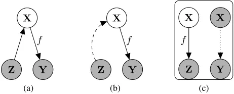
Figure 1: Incorporating uncertain inputsZin GPs through an intermediate input spaceXby considering: (a) a Gaus-sian prior onX, centered on Zand (b) a variational con-straint (dashed line) on the approximate posterior. Figure (c) represents our two-stage approach to dealing with miss-ing outputs for classification, where the dotted line repre-sents a discriminative mapping.

2.1 VARIATIONAL CONSTRAINT

An alternative way of relating the true with the noisy in-puts can be obtained by focusing on the posterior rather than the prior distribution. To start with, we re-express the variational lower bound of equation (5) as:

logp(Y|Z)≥

Z

X

q(X) logp(Y|Z)p(X|Y,Z) q(X) =F

from where we break the logarithm to obtain:

F = logp(Y|Z)−KL(q(X)kp(X|Y,Z)).

We see that the lower bound becomes exact when the vari-ational distributionq(X)matches the true posterior distri-bution of the noise-free latent inputs given the observed puts and outputs. To allow for this approximation we in-troduce a simple variational constraint which operates on the factorised distribution, which is now written asq(X|Z)

where all inputs are observed but uncertain, the constraint just consists of replacing the variational meansµi,:of each

factor q(xi,:)with the corresponding observed inputzi,:.

The variational parametersSi,:then account for the

uncer-tainty. Similarly to the back-constraint of Lawrence and Qui˜nonero Candela [2006]; Ek et al. [2008], our varia-tional constraint does not constitute a probabilistic map-ping. However, it allows us to encode the input noise directly in the approximate posterior without having to specify additional noise parameters or sacrifice scalability. Next, we elaborate on the exact form of the constraint.

In the general case, namely having inputs that are only par-tially observed, we can define a similar constraint which specifies a variational distribution as a mix of Gaussian and Dirac delta distributions. Notationally we consider data to be split into fully and partially observed subsets, e.g.

Z = (ZO

,ZU

), whereO andUdenote fully and partially observed sets respectively. The features missing inZU

can appear in different dimension(s) for each individual point

zU

i,:, but for notational clarityUwill index rows containing

at least one missing dimension. In this case, the variational distribution is constrained to have the form

q(X|Z,{O,U}) =q(XO_|ZO

)q(XU_|ZU

)

=Y

i∈O

N xO

i,:|z

O

i,:, εI

Y

i∈U

N xU

i,:|µ

U

i,:,S

U

i,:

, (6)

whereε → 0, so that the corresponding distributions ap-proximate a Dirac delta. Notice that for a partially observed rowzU

i,:, we can still replace an observed dimensionjwith

its corresponding observation in the second set of factors of equation (6), i.e.µU

i,j = z

U

i,j, soq(X

U_|ZU

) 6= q(XU

). Given the above, as well as a spherical Gaussian prior for

p(X), the required intractable densitylogp(Y|Z) is ap-proximated with a variational lower bound:

F=hlogp(Y|X)iq(X_|Z₎−KL(q(X|Z)kp(X)), (7)

where for clarity we dropped the dependency on {O,U} from our expressions. Since the Dirac functions are ap-proximated with sharply peaked Gaussians inside the pos-terior q(X|Z), the above variational bound can be com-puted in the same manner as the Bayesian GP-LVM bound of equation (3). Specifically, the KL term is tractable, since it only involves Gaussians.

As for the first term of equation (7), we follow the Bayesian GP-LVM methodology and we augment the probability space with m extra samplesU = {ui}mi=1 of the latent

function f evaluated at a set of pseudo-inputs (known as “inducing points”) Xu, so thatU ∈ ℜm×p and Xu ∈

ℜm×q_{. Due to the consistency of GPs,p(U|X}

u)is a

Gaus-sian distribution. From now on we omit dependence onXu

from our expressions. The likelihood then becomes:

p(Y,F,U|X) =p(Y|F)p(F|U,X)p(U).

Then, the marginal p(Y|X) can be obtained from Jensen’s inequality after introducing a variational distribu-tionq(F,U), so thatF ≤ˆ logp(Y|X), where:

ˆ

F=

Z

F,U

q(F,U) logp(Y|F)p(F|U,X)p(U) q(F,U) . (8)

Now the fist term of equation (7) is approxmated as

hp(Y|X)i_q(X_|Z₎ ≥ hFiˆ q(X|Z). However, this

approx-imation is still intractable, since the problematic term

p(F|U,X)still appears inside Fˆ and contains X in the inverse of the covariance matrix, thus rendering the expec-tation intractable. The trick of Titsias and Lawrence [2010] is to define a variational distribution of the form:

q(F,U) =p(F|U,X)q(U). (9)

Replacing equation (9) inside the bound of equation (8) re-sults in the cancellation of p(F|U,X), leaving us with a tractable (partial) bound, which takes the form:

hp(Y|X)i_q(X|Z)≥ hFiˆ q(X_|Z₎=−KL(q(U)kp(U))

+

Z

X,U

q(X|Z)q(U)

Z

F

p(F|U,X) logp(Y|F)

.(10)

The augmentation trick decouples the latent function val-ues given the inducing points, so that any uncertainty in the inputs can be propagated through the nested integral. After this operation, the inducing outputsUcan be marginalised out. Therefore, the above integral is analytically tractable, since the nested integral is tractable and results in a Gaus-sian whereXno longer appears in the inverse of the covari-ance matrix. The final lower bound to use as an objective function is thus obtained by using the partial bound of eq. (10) in place of the first term of equation (7), thus obtaining a new, final bound (more details in the Appendix):

F2=hFiˆ q(X|Z)−KL(q(X|Z)kp(X)). (11)

To summarise, the variational methodology seeks to ap-proximate the true posterior with a variational distribution

q(F,U,X) = q(F)q(U)q(X). To achieve this, q(F)is constrained to take the exact form p(F|U,X). This term is then “eliminated”, giving us tractability, but its effect is re-introduced through the variational distribution (in the nested integral of eq. (10)). Contrast this with the varia-tional constraint onq(X): that approximate posterior fac-tor is constrained according toZ, so that the effect ofZis considered only through theq(X|Z)(eq. (11)). The above comparison gives insight in the conceptual similarity of the variational approach followed to obtain tractability and the one followed for handling partially observed inputs.

The variationally constrained model is shown in fig. 1(b). The total set of parameters to be optimised in the objective functionF2 of equation (11) (e.g. using a gradient-based

optimiser) are the model parameters(θf, β), whereθf

and the variational parameters(Xu,{µUi,:,S

U

i,:}i∈U)(q(U) can be optimally eliminated, see Appendix). Depending on the application and corresponding learning algorithm, cer-tain dimensions of{µU

i,:,S

U

i,:}can be treated as observed.

Such algorithms are discussed in the following sections.

3

GP LEARNING WITH MISSING

VALUES

We formulate both the semi-described and semi-supervised learning as particular instances of learning a mapping function where the inputs are associated with uncertainty. In both cases, we devise a two-step strategy based on our uncertain inputs GP framework, which allows to ef-ficiently take into account the partial information in the given datasets to improve the predictive performance. For brevity, we refer to the framework described in the previ-ous section as avariationally constrained GP, from where a semi-described, an auto-regressive and a semi-supervised GP approach are obtained as special cases, given the algo-rithms that will be explained in this section.

3.1 SEMI-DESCRIBED LEARNING

We assume a set of observed outputs Y that correspond to fully observed inputsZO

and partially observed inputs

ZU

, so thatZ = (ZO

,ZU₎

. To make the correspondence clearer, we also split the observedoutputsaccording to the sets{O,U}, so thatY= (YO

,YU

), but note that both out-put sets are fully observed. We are then interested in learn-ing a regression function from ZtoYby using all avail-able information. Since in the variationally constrained GP the inputs are replaced by distributionsq(XO_|ZO

)and

q(XU_|ZU

), the uncertainty overZU

can be taken into ac-count naturally through this variational distribution. In this context, we formulate a data imputation-based approach which is inspired by self-training methods; nevertheless, it is more principled in the handling of uncertainty.

Specifically, the algorithm has two stages; in the first step, we use the fully observed data subset(ZO

,YO₎

to train an initial variationally constrained GP model which encapsu-lates the sharply peaked variational distributionq(XO_|ZO₎ given in equation (6). Given this model, we can then use

YU

to estimate the predictive posterior1 q(XU_|ZU ) in the missing locations of ZU

(for the observed locations we match the mean with the observations in a sharply peaked marginal, as for ZO

). Essentially, we replace the missing locations of the variational means µU

i,: and variances S

U

i

of q(XU_|ZU

)with the predictive mean and variance ob-tained through the “self-training” step. This selection for

{µU

i,:,S

U

i}constitutes nevertheless only an initialisation. In

1

The predictive posterior for test dataY∗is obtained by max-imising a variational lower bound similar to the training one (eq. (11)), butXandYare now replaced with(X,X∗)and(Y,Y∗).

the next step, these parameters are further optimised to-gether with the fully observed data. Specifically, after ini-tializingq(X|Z) = q(XO

,XU_|Z

)as explained in step 1, we proceed to train a variationally constrained GP model on the full (extended) training set((ZO

,ZU₎

,(YO

,YU₎₎ , which contains fully and partially observed inputs.

Algorithm 1 outlines the approach in more detail. This for-mulation defines asemi-described GPapproach which nat-urally incorporates fully and partially observed examples by communicating the uncertainty throughout the relevant parts of the model in a principled way. Indeed, the predic-tive uncertainty obtained when imputing missing values in the first step of the pipeline is incorporated as input uncer-tainty in the second step of the pipeline. In extreme cases resulting in very non-confident predictions, for example in the presence of outliers, the corresponding locations will simply be ignored automatically due to the large uncer-tainty. This mechanism, together with the subsequent opti-misation of the parameters ofq(XU_|ZU₎

in stage 2, guards against reinforcing bad predictions when imputing missing values based on a smaller training set. The model includes GP regression and the GP-LVM as special cases. In par-ticular, in the limit of having no observed values our semi-described GP is equivalent to the GP-LVM and when there are no missing values it is equivalent to GP regression.

There are some similarities to traditional self-training [Rosenberg et al., 2005], but as there are no straightforward mechanisms to propagate uncertainty in that domain, they typically rely on boot-strapping followed by thresholding “bad” samples to prevent model over-confidence. In our framework, the predictions made by the initial model only constitute initialisations which are later optimised along with model parameters and, hence, we refer to this step as partialself-training. Further, the predictive uncertainty is not used as a hard measure of discarding unconfident pre-dictions; instead, we allow all values to contribute accord-ing to an optimised uncertainty measure, that is, the input variances Si. Therefore, the way in which uncertainty is

handled makes the self-training part of our algorithm prin-cipled compared to many bootstrap-based approaches.

DEMONSTRATION

Algorithm 1Semi-described learning with uncertain input GPs. 1: Given: Fully and partially observed inputs,ZO

andZU

respectively, corresponding to fully observed outputsYO andYU

. 2: Constructq(XO

|ZO ) =Qn

i=1N x O i,:|zOi,:, εI

,where:ε→0

3: Fixq(XO |ZO

)in the optimiser #(i.e.q(XO

|ZO

)has no free parameters) 4: Train a variationally constrained GP modelMO

with inputsq(XO |ZO

)and outputsYO 5: fori= 1,· · ·,|YU

|do

6: Predict the distributionNxU i,:|µˆUi,:,Sˆ

U i

≈p(xU i,:|y

U i,:,M

O

)from the approximate posterior of modelMO .

7: Initialise parameters{µUi,:,SUi}ofq(x U

i,:|zUi,:) =N xi,:U|µUi,:,SUi

as follows: 8: forj= 1,· · ·, qdo

9: ifzi,jU is observedthen

10: µU

i,j =z U i,jand(S

U

i)j,j=ε,where:ε→0

11: FixµU

i,j,(S U

i)j,jin the optimiser #(i.e. they don’t constitute parameters)

12: else

13: µUi,j = ˆµ U i,jand(S

U

i)j,j= (ˆS U i)j,j

14: Train model MO,U _{with inputs}

q(X{O,U}_|Z{O,U}_{) and outputs (Y}O

,YU₎

. The input distribution q(X{O,U}_|Z{O,U}_{) =}

q(XO

|ZO₎

q(XU

|ZU₎

is constructed in steps 2, 5-13 and further optimised in the non-fixed locations.

15: ModelMO,U

now constitutes the semi-described GP and can be used for all required prediction tasks.

inputs. That is, given a partial joint representation of the human body, the task is to infer the rest of the represen-tation. For both datasets, simulated and motion capture, we selected a portion of the training inputs, denoted asZU

, to have randomly missing features. The extended dataset

((ZO

,ZU

),(YO

,YU

))was used to train: a) our method, referred to as semi-described GP (SD-GP) b) multiple lin-ear regression (MLR) c) regression by performing nlin-earest neighbour (NN) search between the test and training in-stances, in the observed input locations d) performing data imputation using the standard GP-LVM. Not taking into account the predictive uncertainty during imputation was found to have catastrophic results in the simulated data, as the training set was not robust against bad predictions. Therefore, the “GP-LVM” variant was not considered in the real data experiment. We also considered: e) a standard GP which cannot handle missing inputs straightforwardly and so was trained only on the observed data (ZO

,YO₎ . The goal was to reconstruct test outputsY∗given fully

ob-served test inputsZ∗. For the simulated data we used the

following sizes: |ZO

| = 40,|ZU

| = 60and|Z∗| = 100.

The dimensionality of the inputs is q = 15 and of the outputs is p = 5. For the motion capture data we used

|ZO_|

= 50,|ZU_|

= 80and|Z∗|= 200. In fig. 2 we plot the

MSE obtained by the competing methods for a varying per-centage offv missing features inZU

. For the simulated data experiment, each of the points in the plot is an average of 4 runs which considered different random seeds. For clarity, they−axis limit is fixed in figure 2, because some methods produced huge errors. The full picture is in figure 5 (Ap-pendix). As can be seen in the figures, the semi-described GP is able to handle the extra data and make much better predictions, even if a very large portion is missing. Indeed, its performance starts to converge to that of a standard GP when there are 90% missing values in ZU

and performs

identically to the standard GP when 100% of the values are missing. We found that whenqis large compared topand

n, then the data imputation step can be problematic as the percentage of missing features inZU

approaches100%i.e. the method is reliant on having some covariates available. Appendix D discusses this behaviour, but a more system-atic investigation is left as future work.

3.2 AUTO-REGRESSIVE GAUSSIAN PROCESSES

Having a method which implicitly models the uncertainty in the inputs of a GP also allows for doing predictions in an autoregressive manner [Oakley and O’Hagan, 2002] while propagating the uncertainty through the predictive sequence [Girard et al., 2003; Qui˜nonero-Candela et al., 2003]. Specifically, assuming that the given dataY consti-tute a multivariate timeseries where the observed time vec-tortis equally spaced, and given a time-window of length

τ, we can reformatYinto input-output collections of pairs

ˆ

ZandYˆ as follows: the first input to the model,ˆz1,:, will

be given by the stacked vector[y1,:, ...,yτ,:]and the first

output,yˆ1,:, will be given byyτ+1,: and similarly for the

other data inZˆ andYˆ, so that:

[ˆz1,:,ˆz2,:, ...,ˆzn−τ,:] =

[y1,:,y2,:, ...,yτ,:],[y2,:,y3,:, ...,yτ+1,:], ...

, [ˆy1,:,yˆ2,:, ...,yˆn−τ,:] = [yτ+1,:,yτ+2,:, ...,yn,:].

To perform extrapolation we first train the model on the modified dataset ( ˆZ,Yˆ). By referring to the semi-described formulation semi-described in Section 3.1, we assign all training inputs to the observed setO. After training, we can perform iterative prediction to find a future sequence

ˆ

Z∗:= [yn+1,:,yn+2,:, ...]where, similarly to the approach

0 20 40 60 80 0.05

0.1 0.15 0.2 0.25 0.3

M

SE

SD−GP

GP NN GPLVM Toy data

0 20 40 60 80

0.2 0.25 0.3 0.35 0.4 0.45 0.5

M

SE

Motion capture data

% missing features % missing features

Figure 2: MSE for predictions obtained by different methods on semi-described learning. GP cannot handle partial ob-servations, thus the uncertainty (2σ) is constant; for clarity, the errorbar is plotted separately on the right of the dashed vertical line (for nonsensicalxvalues). The results for simulated data are obtained from 4 trials. For clarity, the limits on they−axis are fixed, so when the errors become too big for certain methods they get off the chart. The errorbars for the GPLVM-based approach are also too large and not plotted. The full picture is given in figure 5 (Appendix).

step is accounted for and propagated in the subsequent pre-dictions. The algorithm makes iterative 1-step predictions in the future; initially, the outputzˆ1,∗:=yn+1,:will be

pre-dicted (given the training set) with predictive varianceSˆ∗;1.

In the next step, the “observations” set will be augmented to include the distribution of predictions over yn+1,:, by

defining q(xn+1,:|ˆz1,∗) = N

xn+1,:|ˆz∗,1,Sˆ∗;1

, and so on. This simulation process can be seen as constructing a predictive sequence step by step, i.e. the newly inserted in-put points constitute parts of the (test) predictive sequence and not training points. Therefore, this procedure can be seen as an iterative version of semi-described learning.

Note that it is straightforward to extend this model by ap-plying this auto-regressive mechanism in a latent space of a stacked model or, more generally, as a deep GP [Dami-anou and Lawrence, 2013]. By additionally introducing functions that map from this latent space nonlinearly to an observation space, we obtain a fully nonlinear state space model in the manner of Deisenroth et al. [2012]. For our model, uncertainty is encoded in both the states and the nonlinear transition functions. Correct propagation of un-certainty is vital in well calibrated models of future system behavior, and automatic determination of the structure of the model (e.g. the window size) can be informative in de-scribing the order of the underlying dynamical system.

DEMONSTRATION: ITERATIVE FORECASTING

Here we demonstrate our framework in the simulation of a state space model. We consider the Mackey-Glass chaotic time series, a standard benchmark which was also consid-ered by Girard et al. [2003]. The data is one-dimensional so that the timeseries can be represented as pairs of values

{y,t}, t= 1,2,· · · , nand simulates the process:

dζ(t)

dt =−bζ(t) +α

ζ(t−T)

1+ζ(t−T)10,(α, b, T) = (0.2,0.1,17).

Obviously the generating process is very non-linear, ren-dering this dataset challenging. We trained the autoregres-sive model on data from this series, where the modified dataset {zˆ,y}ˆ was created withτ = 18 and we used the first 4τ = 72points to train the model and predicted the subsequent1110points through iterative free simulation.

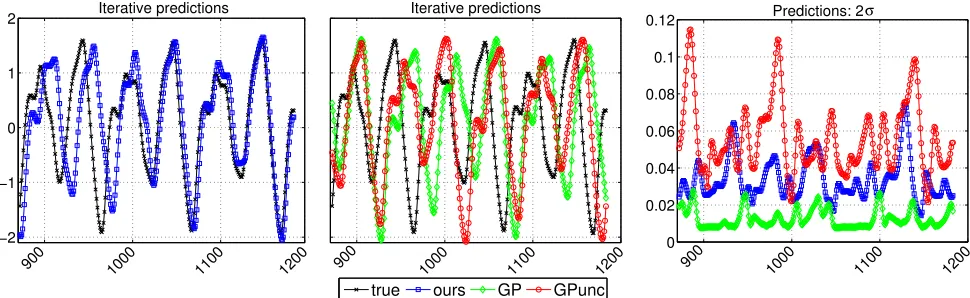
We compared our method with a “naive autoregressive” GP model where the input-output pairs were given by the au-toregressive modification of the dataset {ˆz,y}ˆ . For that model, the predictions are made iteratively and the pre-dicted values after each predictive step are added to the “observation” set. However, this standard GP model has no straight forward way of incorporating/propagating the uncertainty and, therefore, the input uncertainty is zero for every step of the iterative predictions. We also compared against the method of Girard et al. [2003]2, denoted in the plots as “GPuncert”. Figure 3 shows the results for the last

310 steps (i.e. t = 800onwards) of the full free simula-tion (1110−step ahead forecasting); figure 6 (Appendix) gives a more complete picture. As can be seen in the vari-ances plot, both our method and GPuncert are more robust

in handling the uncertainty throughout the predictions; the “naive” GP method underestimates the uncertainty. Conse-quently, as can be seen in figure 6, in the first few predic-tions all methods give the same answer. However, once the predictions of the “naive” method diverge a little by the true values, the error is carried on and amplified due to under-estimating the uncertainty. On the other hand, GPuncert

per-haps overestimates the uncertainty and, therefore, is more conservative in its predictions, resulting in higher errors. Quantification of the error is shown in Table 1 (Appendix).

2

900 _{1000 1100 1200} −2

−1 0 1

2 Iterative predictions

900 _{1000 1100 1200} Iterative predictions

900 _{1000 1100 1200} 0

0.02 0.04 0.06 0.08 0.1

0.12 Predictions: 2σ

true ours GP GPunc

Figure 3: Chaotic timeseries: forecasting1110steps ahead by iterative prediction. The first800steps are not shown here, but figure 6 (Appendix) gives the complete picture. Comparing: a “naive autoregressive” GP which does not propagate (and hence underestimates) the uncertainties; the method of Girard et al. [2003], referred to as GPuncert; and our approach,

which closely tracks the true test sequence until the last steps of the extrapolation. The comparative depiction of the predictions is split into two plots (for clarity), left and center. The rightmost plot shows the predictive uncertainties (2σ).

x−axis is the prediction step (t) andy−axis is the function value,f(t).

3.3 SEMI-SUPERVISED LEARNING

In this section we study semi-supervised learning which, in contrast to semi-described learning, is for handling missing values in the outputs. This scenario is typically encoun-tered in classification settings. Therefore, we introduce the sets {L,M}that index respectively thelabelled and miss-ing (unlabelled) rows of the outputs (labels)Y. Accord-ingly, the full dataset is split so that Z = (ZL

,ZM

)and

Y= (YL

,YM₎

, whereZis now fully observed. The task is then to devise a method that improves classification per-formance by using both labelled and unlabelled data.

Inspired by Kingma et al. [2014] we define a semi-supervised GP framework where features are extracted from all available information and, subsequently, are given as inputs to a discriminative classifier. Specifically, using the whole input spaceZ, we learn a low-dimensional la-tent space X through an approximate posterior q(X) ≈

p(X|Z). Obviously, this specific case where the input space is uncertain but totally unobserved (i.e. a latent space) just reduces to the Bayesian GP-LVM model. No-tice that the posterior q(X)is no longer constrained with

Zbut, rather, directly approximatesp(X|Z), since we now have a forwardprobabilisticmapping fromXtoZandZis treated as a random variable withp(Z|X)being a Gaussian distribution, i.e. exactly the same setting used in the GP-LVM. Since there is one-to-one correspondence between

X,Z andY, we can notationally writeX = (XL

,XM₎ . Further, since we assume thatq(X)is factorised across dat-apoints, we can writeq(X) =q(XL₎

q(XM₎ .

In the second step of our semi-supervised algorithm, we train a discriminative classifier fromq(XL

)to the observed labelled space, YL

. The main idea is that, by including the inputsZM

in the first learning step, we manage to

de-fine a better latent embedding from which we can extract a more useful set of features for the discriminative clas-sifier. Notice that what we would ideally use as input to the discriminative classifier is a whole distribution, rather than single point estimates. Therefore, we wish to take ad-vantage of the associated uncertainty; specifically, we can populate the labelled set by sampling from the distribution

q(XL

). For example, if a latent pointxL

i,: corresponds to

the input-output pair(zL

i,:,y

L

i,:), then a sample fromq(x

L

i,:)

will be assigned the labelyL

i,:.

The two inference steps described above are graphically depicted in Figure 1c. This is exactly the same setting suggested by Kingma et al. [2014], but here we wish to investigate its applicability in a non-parametric, Gaussian process based framework. The very encouraging results reported below point towards the future direction of apply-ing this technique in the framework of deep Gaussian pro-cesses [Damianou and Lawrence, 2013], so as to be able to compare to [Kingma et al., 2014] who considered deep, generative (but nevertheless parametric) models.

DEMONSTRATION

dimen-20 40 60 80 100 120 140 160 20

40 60 80 100 120

# Errors

Oil data

Semi−supervised (using sampling) PCA

# Observed

-# Observed

100 200 300 400 500 600

30 40 50 60 70 80 90 100

D

igits data

Semi−supervised (using sampling) Bayesian GP−LVM

PCA

# Errors

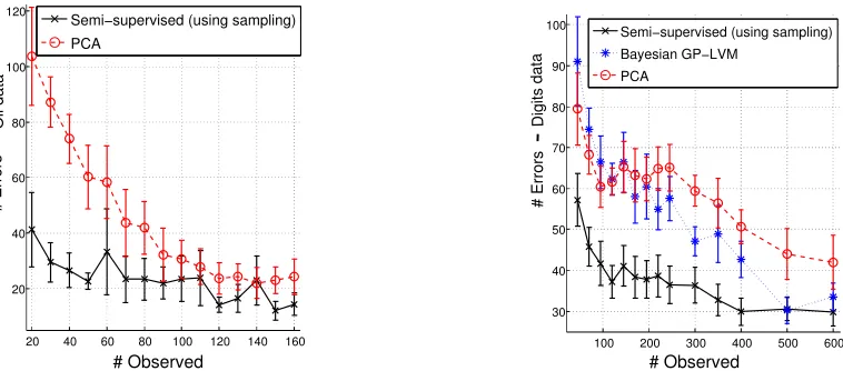
-Figure 4: Plots of the number of incorrectly classified test points as a function of|ZL_|

. Multiple trials were performed, but the resulting errorbars are shown at one standard deviation. In small training sets large errorbars are expected because, occasionally, very challenging instances/outliers can be included and result in high error rates (for all methods) that affect the overall standard deviation. The Bayesian GP-LVM baseline struggled with small training sets and performed very badly in the oil dataset; thus, it is not plotted for clarity.

sional observations belonging to three known classes cor-responding to different phases of oil flow. In each of the 10 performed trials, 700 instances were used as a test set whereas the rest were split to different proportions of la-belled/unlabelled sets. Multi-label data can also be handled by our method, but this case was not considered here.

Our method learned a low-dimensional embedding q(X)

from all available inputs, and a logistic regression classifier was then trained from the relevant parts of the embedding to the corresponding class space. We experimented with taking different numbers of samples fromq(XL₎

for popu-lating the initial labelled set; the difference after increasing over 6 samples was minimal. Also, when using only the mean ofq(XL

)(as opposed to using multiple samples) we obtained worse results (especially in the digits data), but this method still outperformed the baselines. We compared with training the classifier on features learned by (a) a stan-dard Bayesian GP-LVM and (b) PCA, both applied inZL

. Both of the baselines do not takeZM

into account, nor do they populate small training sets using sampling. Figure 4 presents results suggesting that our approach manages to effectively take into account unlabelled data. The gain in performance is significant, and our method copes very well even when labelled data is extremely scarce. Notice that all methods would perform better if a more robust classifier was used, but logistic regression was a convenient choice for performing multiple trials fast. Therefore, our conclu-sions can be safely drawn from the obtained relative errors, since all methods were compared on equal footing.

4

DISCUSSION AND FUTURE WORK

We have defined semi-described learning as the scenario where missing and uncertain values occur in the inputs. We

considered semi-described problems to be part of a general class of missing value problems that also includes semi-supervised learning and auto-regressive future state sim-ulation. A principled method for including input uncer-tainty and partial inputs in Gaussian process models was also introduced to solve these problems within a single, co-herent framework. We explicitly represent this uncertainty as approximate posterior distributions which are variation-ally constrained. This allowed us to further define algo-rithms for casting the missing value problems as particular instances of learning pipelines which use our variationally constrained GP formulation as a building block. Our algo-rithms resulted in significant performance improvement in forecasting, regression and classification. We believe that our contribution paves the way for building powerful mod-els for representation learning from real-world, heteroge-nous data. In particular, this can be achieved by combin-ing our method with deep Gaussian process models [Dami-anou and Lawrence, 2013] that use relevance determination techniques [Damianou et al., 2012], so as to consolidate semi-described hierarchies of features that are gradually abstracted to concepts. We plan to investigate the appli-cation of these models in settings where control [Deisen-roth et al., 2014] or robotic systems learn by simulating future states in an auto-regressive manner and by using in-complete data with miminal human intervention. Transfer learning is another promising direction for applying these models.

ACKNOWLEDGEMENTS

References

C. M. Bishop and G. D. James. Analysis of multiphase flows using dual-energy gamma densitometry and neural networks. Nuclear Instruments and Methods in Physics Research, A327:580–593, 1993.

O. Chapelle, B. Sch¨olkopf, and A. Zien, editors. Semi-supervised Learning. MIT Press, Cambridge, MA, 2006. Z. Dai, A. Damianou, J. Hensman, and N. Lawrence. Gaus-sian process models with parallelization and GPU accel-eration. arXiv preprint arXiv:1410.4984, 2014.

P. Dallaire, C. Besse, and B. Chaib-Draa. Learning Gaus-sian process models from uncertain data. InNeural In-formation Processing, pages 433–440. Springer, 2009. A. Damianou and N. Lawrence. Deep Gaussian processes.

InProceedings of the Sixteenth International Workshop on Artificial Intelligence and Statistics (AISTATS), pages 207–215. JMLR W&CP 31, 2013.

A. Damianou and N. Lawrence. Uncertainty propagation in Gaussian process pipelines. NIPS workshop on modern non-parametrics, 2014.

A. Damianou, M. Titsias, and N. D. Lawrence. Variational Gaussian process dynamical systems. In Advances in Neural Information Processing Systems 24, pages 2510– 2518. 2011.

A. Damianou, C. Ek, M. Titsias, and N. Lawrence. Mani-fold relevance determination. InProceedings of the 29th International Conference on Machine Learning (ICML), pages 145–152. Omnipress, 2012.

M. P. Deisenroth, R. D. Turner, M. F. Huber, U. D. Hanebeck, and C. E. Rasmussen. Robust filtering and smoothing with Gaussian processes. Automatic Control, IEEE Transactions on, 57(7):1865–1871, 2012.

M. P. Deisenroth, D. Fox, and C. E. Rasmussen. Gaus-sian processes for data-efficient learning in robotics and control.IEEE Transactions on Pattern Analysis and Ma-chine Intelligence, 99:1, 2014. ISSN 0162-8828. C. H. Ek, J. Rihan, P. Torr, G. Rogez, and N. D. Lawrence.

Ambiguity modeling in latent spaces. In A. Popescu-Belis and R. Stiefelhagen, editors,Machine Learning for Multimodal Interaction (MLMI 2008), LNCS, pages 62– 73. Springer-Verlag, 28–30 June 2008.

Y. Gal, M. van der Wilk, and C. E. Rasmussen. Distributed variational inference in sparse Gaussian process regres-sion and latent variable models. arXiv:1402.1389, 2014. Z. Ghahramani and M. I. Jordan. Learning from incom-plete data. Technical Report CBCL 108, Massachusetts Institute of Technology, 1994.

A. Girard, C. E. Rasmussen, J. Qui˜nonero Candela, and R. Murray-Smith. Gaussian process priors with uncer-tain inputs—application to multiple-step ahead time se-ries forecasting. InAdvances in Neural Information Pro-cessing Systems, pages 529–536, 2003.

J. J. Hull. A database for handwritten text recognition re-search. IEEE Transactions on Pattern Analysis and Ma-chine Intelligence, 16:550–554, 1994.

D. P. Kingma, D. J. Rezende, S. Mohamed, and M. Welling. Semi-supervised learning with deep generative models. CoRR, abs/1406.5298, 2014.

N. D. Lawrence. The Gaussian process latent variable model. Technical Report CS-06-03, The University of Sheffield, Department of Computer Science, 2006. N. D. Lawrence and M. I. Jordan. Semi-supervised

learn-ing via Gaussian processes. In L. Saul, Y. Weiss, and L. Bouttou, editors, Advances in Neural Information Processing Systems, volume 17, pages 753–760, Cam-bridge, MA, 2005. MIT Press.

N. D. Lawrence and J. Qui˜nonero Candela. Local dis-tance preservation in the GP-LVM through back con-straints. In W. Cohen and A. Moore, editors, Proceed-ings of the International Conference in Machine Learn-ing, volume 23, pages 513–520. Omnipress, 2006. ISBN 1-59593-383-2. doi: 10.1145/1143844.1143909. A. McHutchon and C. E. Rasmussen. Gaussian process

training with input noise. InNIPS, 2011.

J. Oakley and A. O’Hagan. Bayesian inference for the uncertainty distribution of computer model outputs. Biometrika, 89(4):769–784, 2002.

M. Osborne and S. J. Roberts. Gaussian processes for pre-diction. Technical report, Department of Engineering Science, University of Oxford, 2007.

J. Qui˜nonero-Candela. Learning with uncertainty-Gaussian processes and relevance vector machines. PhD thesis, Technical University of Denmark, 2004.

J. Quinonero-Ca˜ndela and S. Roweis. Data imputation and robust training with Gaussian processes. NIPS, 2003. J. Qui˜nonero-Candela, A. Girard, J. Larsen, and C. E.

Ras-mussen. Propagation of uncertainty in bayesian kernel models-application to multiple-step ahead forecasting. InAcoustics, Speech, and Signal Processing, 2003. Pro-ceedings.(ICASSP’03). 2003 IEEE International Con-ference on, volume 2, pages II–701. IEEE, 2003. C. Rosenberg, M. Hebert, and H. Schneiderman.

Semi-supervised self-training of object detection mod-els. In Application of Computer Vision, 2005. WACV/MOTIONS ’05 Volume 1., volume 1, pages 29– 36, Jan 2005. doi: 10.1109/ACVMOT.2005.107. D. B. Rubin. Multiple imputation for nonresponse in

sur-veys, volume 81. John Wiley & Sons, 2004.

M. Titsias and N. D. Lawrence. Bayesian Gaussian pro-cess latent variable model.Journal of Machine Learning Research - Proceedings Track, 9:844–851, 2010. J. Zhu, A. Ahmed, and E. P. Xing. Medlda: maximum