Processes Controlling Tropical Tropopause Temperature and Stratospheric Water Vapor in Climate Models

Stratospheric Water Vapor in Climate Models

.

White Rose Research Online URL for this paper:

http://eprints.whiterose.ac.uk/90158/

Version: Published Version

Article:

Hardiman, SC, Boutle, IA, Bushell, AC et al. (19 more authors) (2015) Processes

Controlling Tropical Tropopause Temperature and Stratospheric Water Vapor in Climate

Models. Journal of Climate, 28 (16). 6516 - 6535. ISSN 0894-8755

https://doi.org/10.1175/JCLI-D-15-0075.1

[email protected] https://eprints.whiterose.ac.uk/ Reuse

Unless indicated otherwise, fulltext items are protected by copyright with all rights reserved. The copyright exception in section 29 of the Copyright, Designs and Patents Act 1988 allows the making of a single copy solely for the purpose of non-commercial research or private study within the limits of fair dealing. The publisher or other rights-holder may allow further reproduction and re-use of this version - refer to the White Rose Research Online record for this item. Where records identify the publisher as the copyright holder, users can verify any specific terms of use on the publisher’s website.

Takedown

If you consider content in White Rose Research Online to be in breach of UK law, please notify us by

Processes Controlling Tropical Tropopause Temperature and Stratospheric Water Vapor

in Climate Models

STEVENC. HARDIMAN,* IANA. BOUTLE,* ANDREWC. BUSHELL,* NEALBUTCHART,* MIKEJ. P. CULLEN,* PAULR. FIELD,* KALLIFURTADO,* JAMESC. MANNERS,* SEANF. MILTON,* CYRILMORCRETTE,* FIONAM. O’CONNOR,* BENJ. SHIPWAY,* CHRISSMITH,* DAVIDN. WALTERS,* MARTINR. WILLETT,* KEITHD. WILLIAMS,* NIGELWOOD,* N. LUKEABRAHAM,1,#JAMESKEEBLE,1AMANDAC. MAYCOCK,1,#

JOHNTHUBURN,@ANDMATTHEWT. WOODHOUSE&

* Met Office, Exeter, Devon, United Kingdom

1_{Centre for Atmospheric Science, Department of Chemistry, University of Cambridge, Cambridge, United Kingdom} #_{National Centre for Atmospheric Science, Cambridge, United Kingdom}

@

College of Engineering, Mathematics and Physical Sciences, University of Exeter, Exeter, United Kingdom

&_{Commonwealth Scientific and Industrial Research Organisation, Aspendale, Victoria, Australia}

(Manuscript received 16 January 2015, in final form 19 May 2015)

ABSTRACT

A warm bias in tropical tropopause temperature is found in the Met Office Unified Model (MetUM), in common with most models from phase 5 of CMIP (CMIP5). Key dynamical, microphysical, and radiative processes influencing the tropical tropopause temperature and lower-stratospheric water vapor concentra-tions in climate models are investigated using the MetUM. A series of sensitivity experiments are run to separate the effects of vertical advection, ice optical and microphysical properties, convection, cirrus clouds, and atmospheric composition on simulated tropopause temperature and lower-stratospheric water vapor concentrations in the tropics. The numerical accuracy of the vertical advection, determined in the MetUM by the choice of interpolation and conservation schemes used, is found to be particularly important. Micro-physical and radiative processes are found to influence stratospheric water vapor both through modifying the tropical tropopause temperature and through modifying upper-tropospheric water vapor concentrations, allowing more water vapor to be advected into the stratosphere. The representation of any of the processes discussed can act to significantly reduce biases in tropical tropopause temperature and stratospheric water vapor in a physical way, thereby improving climate simulations.

1. Introduction

Substantial observed variations in stratospheric water vapor (Rosenlof et al. 2001;Solomon et al. 2010) may have a noticeable impact on lower-stratospheric tem-perature (Forster and Shine 1999;Maycock et al. 2014) and surface climate (Forster and Shine 2002). Although the Intergovernmental Panel on Climate Change Fifth Assessment Report concluded that variations in strato-spheric water vapor were unlikely to have contributed to the recent hiatus in the global mean temperature trend (Flato et al. 2013), they could contribute to decadal changes in global mean surface temperature (Solomon

et al. 2010) and directly impact the stratospheric circu-lation and tropospheric jet streams (Maycock et al. 2013). As well as the direct influence of stratospheric water vapor on radiative balance, water vapor can also have a substantial impact on stratospheric chemistry. Increased water vapor in the extratropical stratosphere can lead to increased polar stratospheric cloud formation and there-fore potentially enhance polar ozone depletion (Toon et al. 1989;Solomon et al. 1986;Kirk-Davidoff et al. 1999). These changes in stratospheric ozone can, in turn, in-fluence surface climate and radiation (Son et al. 2008;

Roscoe and Haigh 2007;Madronich et al. 1995;McKenzie et al. 1999;Hegglin and Shepherd 2009).

Water vapor enters the stratosphere in the tropics, up-welling from the tropical upper troposphere, such that the concentrations of water vapor in an air parcel in the tropical lower stratosphere are predominantly determined

Corresponding author address:Steven C. Hardiman, Met Office Hadley Centre, FitzRoy Road, Exeter, Devon, EX1 3PB, United Kingdom. E-mail: [email protected]

DOI: 10.1175/JCLI-D-15-0075.1

by the coldest temperatures encountered by that air parcel along its pathway into the lower stratosphere (Mote et al. 1996;Holton and Gettelman 2001), the so-called Lagrangian dry point (Fueglistaler et al. 2013;Zahn et al. 2014). In this paper the zonal-mean temperature at the tropical tropo-pause, here referred to as the ‘‘cold point,’’ is used since the Lagrangian dry point cannot be calculated. This cold point is a reasonable proxy for dehydration within the tropical tropopause layer (TTL;Fueglistaler et al. 2009) and vari-ability in the cold point is found to explain much of the variability in lower-stratospheric water vapor concentrations (Fueglistaler and Haynes 2005;Gettelman et al. 2010). A realistic simulation of both surface climate change and stratospheric chemistry therefore relies upon climate models having an accurate representation of tropical tropopause temperature and stratospheric water vapor concentrations.

Climate models represent many processes that have the potential to significantly influence the amount of water vapor entering the stratosphere, either directly or via changes to the tropical tropopause temperature (Fig. 1). Cirrus clouds formed in the tropical tropopause region can significantly reduce water vapor mixing ratios in the lower stratosphere, ‘‘freeze drying’’ the air when the water vapor precipitates in the form of ice particles that grow in size as they descend (Jensen and Pfister 2004). This dehydration occurs as a result of the slow horizontal movement of air into this region of thin widely spread cirrus, and not just because of the deep convection of air through this region. The amount of dehydration occurring as a result of these cirrus clouds, although dominated by the air temperature, is also somewhat sensitive to the microphysical processes controlling the ice crystal number densities, particle size distribution (PSD), and fall speed. Horizontal motion within the TTL can result in this dehydrated air spreading

over large areas (Holton and Gettelman 2001). Deep convection penetrating into the TTL may either hydrate or dehydrate the tropopause layer, depending on how much ice is removed by precipitation and on the vertical profile of relative humidity (Jensen et al. 2007). Radiative forcing from greenhouse gases, particularly from ozone in the lower stratosphere (Lacis et al. 1990), and the numerical accuracy of the vertical advection of potential temperature across the tropopause can also influence the cold-point temperature, as can vertical mixing (Flannaghan and Fueglistaler 2011,2014). Numerical accuracy of the verti-cal advection of moisture can directly influence the water vapor concentrations entering the stratosphere.

Figure 2shows tropical temperature biases, relative to ERA-Interim (hereinafter ERA-I; ECMWF 2011; Dee et al. 2011), found in the state-of-the-art climate models that participated in phase 5 of the Coupled Model In-tercomparison Project (CMIP5; Taylor et al. 2012). Across a majority of the models, there is a similar vertical structure in the temperature bias, consisting of a cold bias of around 1.5 K throughout the troposphere, a warm bias of around 2 K at the tropical tropopause, and a smaller warm bias throughout the lower stratosphere [see also Fig. 1 of

Kim et al. (2013)]. The structure of this bias is discussed further insection 2. The Met Office submissions to CMIP5 suffer qualitatively from the same temperature bias as do the majority of models (Fig. 2), but the magnitude of the warm bias at the tropical tropopause is particularly large in these simulations (around 4 K). The main aim of this paper, using global configurations of the Met Office Unified Model described insection 2, is to understand the effect of processes important for controlling the atmospheric tem-perature and humidity in the region of the tropical tropo-pause in climate models.

A range of sensitivity experiments are carried out, modifying each process in turn. These processes, and their impacts, are described in detail insections 3and4. Although the quantitative results of these sensitivity experiments may be specific to the Met Office model it is anticipated, given the similarity of the temperature biases across CMIP5 models (Fig. 2), that the processes described, and the impacts they can have on the tropical tropopause temperature and stratospheric water vapor concentrations, will be relevant to other models, and hence our results are of general interest. Discussions and concluding remarks are given insection 5.

2. Model description, biases, and simulations

a. Model description

We present investigations using global simulations of the Met Office Unified Model (MetUM), which is an atmosphere model used for numerical weather prediction and climate simulations in both global and limited area

configurations (Cullen 1993; Brown et al. 2012). The MetUM simulations in this study primarily use the Global Atmosphere 6.0 (GA6.0) configuration (Walters et al. 2015, unpublished manuscript) of the Hadley Centre Global Environmental Model, version 3 (HadGEM3). For details of older model versions used, see the refer-ences given inTable 1.

The model simulations are atmosphere–land-only, us-ing prescribed sea surface temperatures and sea ice con-centrations following the protocol of the Atmospheric Model Intercomparison Project (AMIP, now an integral part of CMIP; seeTaylor et al. 2012). They have a hori-zontal resolution of 1.8758(longitude)31.258(latitude), corresponding to a resolution of approximately 135 km in the midlatitudes. There are 85 model levels, 50 of which are in the troposphere, with the model upper boundary at 85 km from the surface. In the TTL (;11–17 km), the spacing between model levels ranges from 500 to 700 m. The majority of the sensitivity experiments detailed in the following sections use GA6.0 as their baseline and were run for 20 years in present-day conditions (1989–2008), with the first 10 years discarded as spinup.

Here, specific details on the model’s representation of the processes described inFig. 1are provided, and the reader can refer to Walters et al. (2015, unpublished manuscript) for further details. The model uses a semi-implicit, semi-Lagrangian formulation to solve the nonhydrostatic, fully compressible deep-atmosphere equations of motion (Wood et al. 2014). For tempera-ture and moistempera-ture the model uses variables of virtual po-tential temperature and mass mixing ratios of vapor and hydrometeors. A cubic Lagrange horizontal interpolation to the semi-Lagrangian departure points is used, while in the vertical a cubic Hermite interpolation for potential temperature and quintic Lagrange interpolation for the moist variables are used. The radiation scheme is de-scribed inEdwards and Slingo (1996)and Cusack et al. (1999). Shortwave (SW) radiative transfer uses six bands and models interactions with water vapor (H2O), ozone

(O3), carbon dioxide (CO2), and oxygen (O2). Longwave

(LW) transfer uses nine bands and models interactions with H2O, O3, CO2, methane (CH4), nitrous oxide (N2O), FIG. 2. Bias with respect to ERA-I in annual-mean tropical

tem-perature area averaged from 108S to 108N for all CMIP5 models for which data were available in the central archive. Shown are 10-yr climatologies for the period 1990–99. Individual model biases are shown as thin blue lines, with the multimodel mean plotted as a thick red line. The versions of the MetUM used in CMIP5 (HadGEM2; see

Table 1) are shown as thin green lines. The gray shading indicates the intermodel standard deviation about the multimodel mean.

TABLE1. Versions of the MetUM.

Model name References

Hadley Centre Coupled Model, version 3 (HadCM3) Pope et al. (2000);Collins et al. (2001)

Hadley Centre Global Environment Model, version 1 (HadGEM1) Martin et al. (2006);Hardiman et al. (2010)(stratosphere resolving version)

Hadley Centre Global Environment Model, version 2 (HadGEM2) Martin et al. (2011);Jones et al. (2011)

HadGEM3, Global Atmosphere 3.0 (GA3.0) configuration Walters et al. (2011)

HadGEM3, Global Atmosphere 4.0 (GA4.0) configuration Walters et al. (2014)

chlorofluorocarbon (CFC)-11 (CCl3F), CFC-12 (CCl2F2),

and hydrofluorocarbon (HFC) 134a (CH2FCF3). The

precipitation/microphysics scheme is based on Wilson and Ballard (1999). Large-scale clouds are modeled through the prognostic cloud fraction and prognostic condensate (PC2) scheme (Wilson et al. 2008) with modifications described in Morcrette (2012). This in-cludes water vapor, liquid, and ice cloud condensate as well as separate variables for liquid, ice, and mixed-phase cloud fraction. Finally, the convection scheme uses a mass flux formulation based onGregory and Rowntree (1990)

with various extensions to include downdrafts (Gregory and Allen 1991) and convective momentum transport.

b. Model biases

Although this study focuses primarily on the model temperature bias in the tropical tropopause region, it was shown in the introduction how this bias relates to the tropical temperature bias throughout the depth of the troposphere and stratosphere. Figure 3 shows that all versions of HadGEM, and indeed the older-generation HadCM3 configuration of the MetUM (see Table 1), have suffered qualitatively from the same temperature bias throughout the troposphere and lower stratosphere in the tropics as is found in the majority of the CMIP5 models. This bias is shown relative to ERA-I, but it can be seen that qualitatively the same bias is found rela-tive to the Modern-Era Retrospecrela-tive Analysis for Re-search and Applications (MERRA; Global Modeling

and Assimilation Office 2011;Rienecker et al. 2011), and that the agreement between ERA-I and MERRA is within 61 K at most altitudes. Furthermore, ERA-I is found to agree very well with the Radiosonde Innovation Composite Homogenization (RICH)-adjusted radiosonde temperature data (Haimberger et al. 2012, 2013) at 100 hPa, and so might be considered as close to the ‘‘truth’’ at this altitude as can currently be obtained. The fact that the vertical profile of this temperature bias is qualitatively similar across all versions of HadGEM, and across the CMIP5 models, suggests that the causes for the bias may be common across these models (Kim et al. 2013).

In numerical models, the cold-point temperature is not solely responsible for the stratospheric water vapor concentrations. Biases in tropical stratospheric water vapor are shown inFigs. 4a and 4bfor the most recent versions of HadGEM3, and in Fig. 4c for the CMIP5 models. The biases are shown relative to MERRA (Rienecker et al. 2011), which assimilates water vapor data from both the Halogen Occultation Experiment (HALOE;Russell et al. 1993) and theAuraMicrowave Limb Sounder (MLS; Waters et al. 2006). Although most of these models suffer from a warm bias in tropical tropopause temperature, the CMIP5 models do not, on average, show a moist bias in the stratospheric water vapor, and if anything appear slightly dry in the strato-sphere. It is likely, then, that there are many processes influencing stratospheric water vapor in the CMIP5 cli-mate models—some by altering upper-tropospheric water vapor concentrations directly, which will then be advected by the model into the lower stratosphere as a result of the approximations inherent in the model vertical advection scheme (regardless of the cold-point temperature; see section 3), and some by altering the cold-point temperature and therefore indirectly influ-encing stratospheric water vapor concentrations.

The dipolar nature of the temperature bias in the upper troposphere and lower stratosphere suggests that this bias is related to the model incorrectly simulating the height of the tropopause.Figure 5ashows that the height of the cold point is, accurate to within the vertical resolution of the output data, at 100 hPa. Figure 5b

shows the ‘‘thermal tropopause’’ defined, convention-ally, as the height at which the lapse rate,2dT/dz(where

Tis temperature andzis geometric height), drops below the value 2 K km21 (WMO 1957). Comparing Fig. 5b

withFig. 3demonstrates that the bias in the height of the tropopause is indeed strongly related to the magnitude of the dipole in the temperature bias in the upper tro-posphere and lower stratosphere. Therefore, any pro-cess reducing the magnitude of a model temperature bias in the TTL region also has the potential to reduce any bias in the modeled tropopause height.

For the remainder of the paper, we will focus on the tropical temperature at 100 hPa (area averaged from 108S to 108N) as a measure of the cold-point tempera-ture. We also use specific humidity q at 70 hPa (area averaged from 108S to 108N) as a measure of water vapor concentrations entering the stratosphere in the tropics. An altitude of 70 hPa is within the stratosphere, avoiding the complications of vertical mixing across the cold point that would arise from consideringqat 100 hPa. It is also below the height of the majority of water vapor production by stratospheric oxidation of methane, and no other local processes in the tropical stratosphere are believed to influence stratospheric water vapor con-centrations. Of course, the horizontal mixing of extra-tropical air into the tropics can still influence extra-tropical water vapor concentrations at 70 hPa.

c. Sensitivity experiments

Sensitivity experiments, modifying numerical, micro-physical, and radiative processes, were carried out from a common baseline (GA6.0). The experiments having a significant impact on cold-point temperature and strato-spheric water vapor are summarized inTable 2, and are

referred to below using the names given in Table 2. While some of these sensitivity experiments represent improvements to the model physics and some are simply a modification of model parameters, they all represent a change in the model representation of a process that has an impact on tropical tropopause temperature and/or stratospheric water vapor. Sensitivity experiments were also carried out in which the magnitude of nonorographic gravity wave drag was altered, with the aim of modifying the strength of the stratospheric Brewer–Dobson circu-lation (Butchart 2014), known to impact the cold-point temperature (Gettelman et al. 2010;Dessler et al. 2014). However, in HadGEM3 this was found to have very little impact on the tropopause temperature or water vapor biases, and so, along with other sensitivity experiments having insignificant impact (detailed insection 5), this is not considered further.

As previously discussed, one way to influence lower-stratospheric water vapor in the model is to change the cold-point temperature. In the real atmosphere, the water vapor in a fluid parcel in the lower stratosphere will be determined by the lowest saturation vapor mixing ratio encountered on its route there (Gettelman et al. 2010).

This behavior is incorporated into HadGEM3 using the Goff–Gratch formulation for the saturation water vapor pressure (Goff 1965). The modeled water vapor concen-trations in the lower stratosphere will depend not only upon this formulation, but also on the fact that not all air is fully dehydrated as it passes through the TTL and, fur-thermore, on the approximations inherent in the model advection and parameterization schemes (seesections 3

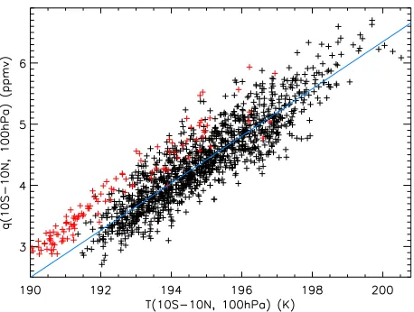
and4below). Furthermore, the saturation vapor mixing ratio is a nonlinear function of temperature, and so the zonal-mean monthly mean temperature at 100 hPa, area averaged from 108S to 108N, being used in this study as a measure of the cold-point temperature, is clearly just a proxy for the temperature at the times and locations where the air in the lower stratosphere will have been saturated (Fueglistaler and Haynes 2005).1Therefore, the following approach is taken to attempt to determine when a change in the modeled lower-stratospheric water vapor concen-tration is almost entirely due to a change in the cold-point temperature.Figure 6shows monthly mean zonal-mean values ofT(108S–108N, 100 hPa) andq(108S–108N, 100 hPa), plotted against each other for every month of every simulation considered in this paper.2 These points are

found to fit very closely to a straight line (Fig. 6), the gradient of which is 0.39 ppmv K21in the model simula-tions (as compared to 0.41 ppmv K21in ERA-I). In what follows, this gradient is referred to as the empirically derived Clausius–Clapeyron relation (for HadGEM3). Physical processes that lead to changes in the cold-point temperature and lower-stratospheric water vapor fol-lowing this empirical relationship are considered to have changed the lower-stratospheric water vapor concentra-tions solely by changing the cold-point temperature. Those that do not follow this relationship are considered to have directly impacted the stratospheric water vapor concentrations.

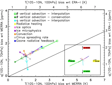
Figure 7shows the effect of the processes detailed in

Table 2 on both the cold-point tropical tropopause temperature (Tat 100 hPa, area averaged from 108S to 108N) and the lower-stratospheric water vapor concen-tration (qat 70 hPa, area averaged from 108S to 108N), averaged over the period 1999–2008.Figure 7shows the biases in temperature and water vapor relative to both MERRA and ERA-I. The differences between the re-analyses give an indication of the uncertainty in the true value of both quantities, but both reanalyses are in good agreement with observations [seeFig. 3, which shows a comparison to the RICH-adjusted temperature dataset, and the top left-hand panel of Fig. 4 inHegglin et al. (2013), which shows the multimodel mean value for zonal-mean water vapor over the period 1998–2008, inferred from several satellite datasets]. A positive bias exists relative to both reanalyses in both temperature and water vapor. It can be seen that theuvertical advection–interpolation,uvertical advection–conservation, radiative heating, ice optics, and ozone radiative feedback processes, which influence tem-perature alone (either through advection or via the radiation scheme) follow the empirically derived Clausius–Clapeyron

FIG. 5. (a) Annual-mean tropical temperature area averaged from 108S to 108N in the different configurations of the MetUM (seeTable 1) and the reanalyses ERA-I and MERRA. For the resolution of output data available, the cold-point temperature is found to be located at 100 hPa. (b) Thermal lapse rate, calculated as2dT/dz(K km21_{), for} the models, ERA-I, and MERRA. The thermal tropopause is defined as the height at which the lapse rate drops to values below 2 K km21

(shown by thin vertical black line).

1

However, the model’s representation of variability in temper-ature at 100 hPa is found to be realistic. The standard deviation of the simulated daily temperatures at 100 hPa differs from ERA-I by only around60.4 K (not shown).

2_{This empirical relationship needs defining usingq(10}

relation very closely, as expected. However, the other processes (qvertical advection–interpolation, ice micro-physics, convection, and cirrus spreading rate) directly influence the water vapor concentrations in the upper troposphere, and do not follow this relation at all. The following sections describe the processes represented in

Fig. 7 in more detail, giving mechanisms for their in-fluence on tropical tropopause temperature and strato-spheric water vapor, and explaining how water vapor concentrations in the upper troposphere can have just as much influence on lower-stratospheric water vapor in the model as can the cold-point temperature.

3. Numerical accuracy of vertical advection in the tropical tropopause layer

The tropopause is characterized by a rapid change in the vertical gradient of potential temperature. In the tropics, the vertical wind in the vicinity of this persistent thermal structure has a very small mean ascent [less than 1 mm s21

on the annual mean; see Fig. 1a ofHardiman et al. (2014)]. Superposed on this mean ascent are wavelike motions with vertical velocities much larger than the mean (Orbe et al. 2012), but whose time scale is short enough for diabatic effects and mixing to be negligible, making them essen-tially physically reversible. Model performance in this re-gion is consequently sensitive to how well the vertical advection scheme performs under such flow conditions.

In a model using a semi-Lagrangian (SL) advection scheme, interpolation of model fields to trajectory departure points is required. The model evolution is therefore sensitive to the polynomial used for this interpolation, and to the set of points used to fit this polynomial (known as the interpolation ‘‘stencil’’).

In HadGEM3, a SL scheme with bicubic Lagrange interpolation is used for horizontal advection. Therefore,

it is desirable to use a cubic scheme also for the vertical advection. However, the SL advection algorithm tradi-tionally chosen, using a four-point cubic Lagrange in-terpolation stencil (Staniforth and C^oté _{1991), only} provides first-order temporal accuracy in the tropopause region because the interpolation stencil shifts with the direction of the vertical wind (seeFig. 8). For upward advection at the tropopause, the interpolation stencil has more points in the troposphere than the stratosphere whereas for downward advection the interpolation stencil contains more stratospheric points than tropospheric

FIG. 6. Sensitivity ofq(108S–108N, 100 hPa) to changes inT(108S– 108N, 100 hPa), as determined from values of monthly mean zonal-meanqandTfor all months from 1999–2008 for all model integrations included in this study (black plus signs) and ERA-I (red plus signs). There are 10 model integrations included (one control and one for each of the nine processes listed inTable 2) and therefore 103103

1251200 model values shown, and 103125120 values shown for ERA-I. The blue line shows the linear least squares fit to the model values, and has a gradient of 0.39 ppmv K21_{(the equivalent gradient} for ERA-I is 0.41 ppmv K21_{, not shown).}

TABLE2. Sensitivity experiments.

Process name Modifications to model

uvertical advection–interpolation Interpolation in vertical advection scheme for potential temperature changed from cubic Lagrange to cubic Hermite.

uvertical advection–conservation Priestley conservation algorithm is applied to interpolated potential temperature in vertical advection scheme.

qvertical advection–interpolation Interpolation in vertical advection scheme for moisture changed from quintic Lagrange to cubic Hermite.

Radiative heating An improved representation of gaseous absorption.

Ice optics An improved representation of the optical properties of atmospheric ice crystals. Ice microphysics An improved representation of the ice particle size distribution and fall speeds of ice

crystals.

Convection Improvements to the vertical transport of heat and moisture by the convective parameterization.

Cirrus spreading rate Change the rate at which unresolved motions act to spread cirrus cloud in the horizontal. Ozone radiative feedback Interactively simulated ozone passed to model radiation scheme, instead of prescribed

ones (Fig. 8). As a result the upward advection is pre-dominantly affected by the tropospheric gradient of po-tential temperature, while the downward advection is dominated by the stratospheric gradient. The stratospheric potential temperature gradient is systematically larger than the tropospheric gradient. Hence there is a lack of cancel-lation between the upward (cooling) and downward (warming) phases of vertical advection, breaking the re-versibility and resulting in a net warming at the tropopause. Cubic Hermite interpolation (Williamson 1990) re-moves this dependence on the direction of the vertical wind by constructing a cubic polynomial from two values of the function and its derivative collocated at two distinct points. When used for SL advection, numerical approxi-mations are required to provide the derivatives. If these derivative approximations are constructed with a sym-metric (centered) stencil, then the SL scheme will assign a single value for the derivative at each grid point, regard-less of the wind direction. Consequently, the SL scheme with cubic Hermite interpolation has second-order

temporal accuracy for small oscillations at the tropo-pause. Using cubic Hermite for the vertical advection of potential temperature thus reduces the spurious heating of the tropopause associated with the cubic Lagrange scheme, significantly reducing the warm bias in the tropical tropopause temperature (seeFig. 9). The tem-perature bias is reduced by 2.25 K (compared to using cubic Lagrange interpolation) and in line with the em-pirically derived Clausius–Clapeyron relation the water vapor bias is reduced by 0.90 ppmv (light green line in

Fig. 7). These changes are statistically significant at the 95% level (as are all changes inFig. 7with the exception of three, as noted in the figure caption). For this reason, cubic Hermite interpolation for potential temperature was included in GA6.0 (i.e., this is the only change shown inFig. 7that does not start from GA6.0).

The vertical advection scheme applied to moisture will also influence the model biases (Stenke et al. 2008). Re-placing quintic Lagrange with cubic Hermite interpola-tion for the vertical advecinterpola-tion of moisture results in a significant reduction in the stratospheric water vapor bias of 0.81 ppmv (light blue line inFig. 7). A further numerical consideration, affecting the choice of vertical advection scheme for water vapor, is the way in which this scheme is coupled to the cloud microphysical processes discussed in

section 4b. These processes are treated as source terms evaluated at the departure points of the SL advection scheme. In the tropopause layer, where freeze-drying is taking place, the amount of water vapor available for ascent is largely determined by a combination of ice

FIG. 7. The effects of different processes on the model biases in annual-mean tropical temperatureTat 100 hPa area averaged from 108S to 108N, and water vaporqat 70 hPa area averaged from 108S to 108N, with respect to MERRA and ERA-I. The direction of the arrows shows the changes due to these processes as described in

sections 3and4. Ten-year climatologies for the period 1999–2008 are used. Apart fromuvertical advection–interpolation (marked by a light green square) all other changes (marked by asterisks) are relative to GA6.0 (marked by a black triangle). The thin black line shows the derived sensitivity ofqtoTin model simulations (gradient of blue line inFig. 6). All the changes toTandqdue to these pro-cesses are statistically significant at the 95% level (using a Student’s

ttest), with the exception of the changes toTbecause ofqvertical advection–interpolation, convection, and cirrus spreading rate. The value ofT(108S–108N, 100 hPa) in ERA-I is 192.4 K and in MERRA is 193.1 K. The value ofq(108S–108N, 70 hPa) in ERA-I is 3.49 ppmv and in MERRA is 3.74 ppmv. The ‘‘observed’’ value ofq(108S–108N, 70 hPa), inferred from the SWOOSH dataset (NOAA/Earth Systems Research Laboratory 2014), is 3.76 ppmv.

microphysics and the Clausius–Clapeyron equation. Advection schemes that interpolate by fitting a poly-nomial over several vertical model levels will inevitably incorporate information about the water vapor saturation vapor mixing ratios at model levels below and above the cold point, as well as at the cold point itself. The resulting saturation vapor mixing ratio determining water vapor concentrations on entry to the stratosphere is thus influenced by water vapor concentrations in the upper troposphere and not just at the cold point (i.e., there is a spatial smoothing of the saturation vapor mixing ratio), potentially weakening the tight coupling be-tween stratospheric water vapor concentrations and cold-point temperature derived inFig. 6. Analysis (C. Smith et al. 2015, unpublished manuscript) shows that the cubic Hermite scheme has lower spatial smoothing in this respect than does the quintic (or cubic) Lagrange

scheme, leading to more realistic stratospheric water vapor concentrations.

Further support for the benefit of the cubic Hermite interpolation method is given inFig. 10, which shows the time evolution of the vertical profile of water vapor area averaged from 108S to 108N, demonstrating the so-called tape-recorder (Mote et al. 1996) effect. The seasonal cycle in the cold-point temperature imposes a seasonal cycle in the stratospheric water vapor concentrations, which is advected upward through the tropical strato-sphere, allowing the mean ascent rate there to be di-agnosed from the slope of the tape-recorder plots. Comparing to observed water vapor inferred from the Stratospheric Water and Ozone Satellite Homogenized dataset (SWOOSH; NOAA/Earth Systems Research Laboratory 2014), it is found that using cubic Hermite vertical interpolation for moisture as well as for potential

temperature gives not only a better mean water vapor concentration throughout the stratosphere, but also a more coherent tape-recorder signal in the midstratosphere.

Improvements have therefore been made by using the same interpolation scheme for the advection of moisture and potential temperature. However, for reasons that have evolved as the model has developed, differences between how moisture and potential temperature are advected remain. Specifically, a mass-conserving algo-rithm (Priestley 1993) is applied to the interpolated moisture mixing ratios to ensure that the corrected in-terpolated values preserve the global integral of mois-ture. This is because interpolation of the mixing ratios does not, except in very special circumstances, preserve mass integrals of the advected quantity. However, in GA6.0 this procedure is not applied to potential tem-perature despite the fact that analytically the product of dry mass and potential temperature is a conserved quantity (for adiabatic flows). In the spirit, then, of

striving to transport moisture and potential temperature in a consistent way, an experiment (labeled ‘‘uvertical advection–conservation’’ in Table 2) was conducted in which the mass-conserving algorithm (Priestley 1993) is also applied to potential temperature. The impact of this change is indicated by the dark green line inFig. 7. There is a clear reduction of both the temperature and humidity biases (of 0.79 K and 0.36 ppmv respectively) in the re-gion of the tropical tropopause. It seems likely that the errors in conservation of potential temperature are preferentially committed where the gradient of potential temperature changes most rapidly (i.e., there is a lack of smoothness in the vertical potential temperature profile). The tropical tropopause is such a location (seeFig. 9).

4. Physical processes in the tropical tropopause layer

The main physical mechanism by which the temper-ature of the TTL is determined is radiative heating by

FIG. 10. Tropical ‘‘tape recorder’’ of monthly mean specific humidityq(ppmv) area averaged from 108S to 108N in (a) SWOOSH, (b) GA6.0 (cubic Hermite vertical interpolation for potential temperature and quintic Lagrange vertical interpolation forq), and (c) GA6.0 with cubic Hermite applied toq(as well as potential temperature). For the period 1999–2005, the SWOOSH dataset is a merged product of HALOE data (Russell et al. 1993) andAuraMLS (Waters et al. 2006), with HALOE data being bias corrected to match the

ozone, water vapor, and carbon dioxide. This radiative heating occurs from both shortwave radiation (direct from above or reflected from below) and longwave ra-diation emitted from the troposphere and surface below. Therefore, the temperature can be modified either by changing the radiation parameterization directly, chang-ing the physical properties of the troposphere that affect upwelling longwave radiation (mainly clouds), or chang-ing the atmospheric concentrations of ozone, water vapor, and carbon dioxide.

The water vapor concentration of the lower strato-sphere is determined by the vertical transport of water vapor from the tropical troposphere. Changes to the cold-point temperature (as discussed insection 2c) or to the water vapor concentration in the upper troposphere (as discussed in the previous section) can modify water vapor concentrations in the lower stratosphere. Water vapor concentrations in the upper troposphere can be modified by changes to the parameterized vertical transport of water through the troposphere (i.e., by convection and precipitation), as discussed below.

a. Radiation changes

Developments beyond GA6.0 include two changes to the radiation scheme that improve the physical basis of the scheme with respect to recent observational and theoretical results.

1) RADIATIVE HEATING

First, the treatment of gaseous absorption has been modified based on the high-resolution transmission molecular absorption database (HITRAN 2012; see

Rothman et al. 2013). This makes use of new

correlated-ktechniques (J. Manners 2015, unpublished manuscript) to improve the scaling of absorption with pressure and temperature leading to an improved representation of stratospheric heating or cooling (resulting from water vapor, ozone, and carbon dioxide). The consequence of this is that more radiation (both longwave and short-wave) is absorbed by stratospheric gases, leading to a direct heating of the tropical tropopause and a 0.74-K tem-perature increase. This temtem-perature increase directly leads to a humidity increase, in line with Clausius–Clapeyron, which is advected upward into the stratosphere, result-ing in a 0.32 ppmv increase in humidity (yellow line in

Fig. 7).

2) ICE OPTICS

Second, a new treatment of the cirrus bulk optical properties based onBaran et al. (2014)is included. An ensemble of ice crystal shapes with known single-scattering properties is used by the microphysics pa-rameterization scheme. These are distributed over the

ice particle size distribution to calculate the bulk optical properties in each grid box. This removes the strong temperature dependence that characterized the pre-vious scheme (Edwards et al. 2007), which was based on directly parameterizing the ice-crystal effective di-ameter as a function of temperature.

For cold tropical cirrus clouds (between temperatures of 210 and 235 K) the inclusion of this new scheme leads to a reduction in longwave absorption. At near-infrared wavelengths the single scattering albedo of ice has also been significantly reduced, leading to increased short-wave absorption (by around 30%) and reduced re-flection from these cold high clouds. The reduction in longwave extinction within the cirrus clouds leads to an increase in upwelling longwave radiation originating from the warmer layers below the cloud. This in turn leads to a relative increase in the heating at the level of the tropical tropopause, as the increased radiation is absorbed by stratospheric gases. This effect dominates over the reduction in upwelling near-infrared radiation reflected from the cloud top. The tropical tropopause temperature is increased by 0.86 K, with a corresponding increase of 0.38 ppmv in humidity, again dominated by the Clausius–Clapeyron relation (pink line inFig. 7).

b. Ice cloud changes

The distribution of high ice cloud influences TTL conditions in two ways. It indirectly affects the temper-ature structure of the layer because of the interaction of ice crystals with solar and terrestrial radiation (Dinh and Fueglistaler 2014). The mechanism for this is identical with that described above when changing the optical properties of the ice cloud, except that we are now changing the concentration, location and extent of the ice cloud. However, it has a direct effect on the humidity structure of the layer because ice cloud acts as a sink of water vapor. Therefore ice cloud changes can potentially affect the stratospheric water vapor in ways different from those predicted by Clausius–Clapeyron arguments. Three changes are discussed which affect the concentra-tion, locaconcentra-tion, and extent of the ice cloud.

1) ICE MICROPHYSICS

The main microphysical processes controlling high cloud are particle sedimentation and depositional growth. Modeling these processes requires assumptions about the ice PSD, fall speeds, and mass–diameter re-lationship. In GA6.0 these properties are either based on antiquated in situ datasets, known to suffer from systematic errors, or have been arbitrarily tuned.

(2015)]. The main benefit, in terms of physical realism, comes from using measurements that have been cor-rected, as far as possible, for contamination by artifacts caused by ice crystal fragmentation on the housings of airborne instrumentation (‘‘shattering’’; Korolev and Isaac 2005,Field et al. 2006). Sensitivity experiments reported inFurtado et al. (2015)showed that the effect of these combined changes is to increase the amount of high cloud, further humidify the TTL, warm the tropo-sphere, and cool the lower stratosphere. These effects can be qualitatively understood as follows.

The parameterization changes reduce the ice crystal fall speeds compared to GA6.0. This significantly decreases the mean sedimentation flux of ice, which causes an in-crease in the amount of high cloud. This effect can be viewed as a consequence of total water conservation: convection and resolved dynamics transport water (vapor and condensate) vertically upward and, in steady-state conditions, this is balanced by downward sedimentation of ice crystals. If a parameterization change decreases the ice sedimentation flux while the upward water flux remains the same, then the ice water content will increase until sedimentation rebalances the upward water transport.

An effect of the PSD change is to increase the char-acteristic time scale for depositional growth of ice. At low temperatures the GA6.0 PSD apportions a large fraction of any given population of ice crystals to sizes less than 100mm. These small crystals provide a very efficient sink of water vapor. Relatively fewer small particles with the PSD change implies that depositional growth occurs less rapidly, allowing the amount of water vapor in the TTL to build up to higher levels. The combination of PSD and fall speed changes results in a 0.22 ppmv increase in stratospheric water vapor, shown by the purple line inFig. 7.

The effect of increased ice cloud on the temperature structure of the TTL and troposphere is determined by cloud-radiative effects, as discussed previously (see alsoSeiki et al. 2015).Figure 11shows the zonal-mean tropical temperature change due to the microphysics changes. The climate response has a dipolar structure in the vertical: tropospheric warming, because of in-tensification of the infrared–greenhouse gas forcing, is accompanied by a cooling of the cold point (of 0.44 K) that extends well into the lower stratosphere, because of reduced infrared transmission to the TTL region and gaseous absorption. Comparison withFig. 3shows that these changes improve the model climatology, both in the troposphere and in the stratosphere.

2) CONVECTION

The convective parameterization is the main mecha-nism in the troposphere by which heat and moisture are

transported vertically in the tropics, and typically it takes warm, moist air from near the surface and dis-tributes it throughout the troposphere. In GA6.0, the convective parameterization had a tendency not to convect high enough into the upper troposphere. This was found to be partly due to numerical approxima-tions made in calculaapproxima-tions of air parcel properties during the parcel ascent.3Therefore, this aspect of the scheme was improved with the consequence that the scheme carries more buoyancy and can penetrate fur-ther into the TTL.

This has two consequences for TTL temperatures. First, the direct detrainment of cirrus cloud from the convective plume occurs at a higher altitude, bringing the modeled cloud height closer to observations (seeFig. 12). Therefore, the cloud tops are colder, and thus emit less longwave radiation into the TTL region, directly reducing the radiative heating. Second, the increased moisture carried by the convective plume means that the detrained cloud contains a greater mass concentration of ice. In exactly the same manner as reducing the sedimentation rate of ice crystals reduced the TTL temperature, in-creasing the source of ice has the same effect.

Early versions of the improved convective parame-terization had a significantly detrimental effect on the stratospheric water vapor, because of the increased moisture carried upward by the convective plume. Once deposited in the upper troposphere, this increased

FIG. 11. Zonal annual-mean structure of the temperature dif-ferences (K) in the tropics induced by the changes to the ice mi-crophysics parameterizations for the period 1999–2008. Contours show temperature difference from GA6.0.

moisture will act, via the interpolation routines in the vertical advection scheme, to increase the water vapor concentration in the lower stratosphere. In fact, this impact, detrimental to GA6.0 and seen because of im-proving the height of convection, was a result of re-moving one of two canceling errors. The MetUM uses an ‘‘adaptive detrainment’’ parameterization as described inDerbyshire et al. (2011). As a rising convective plume detrains material to the surrounding environment, it loses buoyancy. The adaptive detrainment parameteri-zation dictates that much of the material detrained is selectively that which is already neutrally buoyant with respect to the surroundings, such that the loss of buoy-ancy by the plume will be less than otherwise expected and the plume will rise higher. Because of its tendency not to convect high enough, the adaptive detrainment parameterization in GA6.0 was tuned so that very large fractions of neutrally buoyant material were detrained— notably, greater fractions than were considered realistic byDerbyshire et al. (2011). With the improvements al-ready discussed naturally making the plume more buoy-ant, it is no longer necessary to detrain such high fractions of neutrally buoyant material, allowing the adaptive de-trainment parameterization to be used within the bounds recommended byDerbyshire et al. (2011). The net effect of improving the height of convection and the modifica-tion of the adaptive detrainment parameterizamodifica-tion is to increase the lower-stratospheric water vapor concentra-tion by 0.30 ppmv and reduce the cold-point temperature

by 0.15 K (orange line in Fig. 7). Furthermore, these modifications have the additional benefit of significantly improving the tropical precipitation (distribution and amount) in all seasons (not shown).

3) CIRRUS SPREADING RATE

In GA6.0, any ice cloud cover is assumed to gradually spread out, driven by unresolved horizontal mixing within a grid box. In the absence of additional sources, this increases the gridbox mean cloud cover while keep-ing the ice water content constant. The precise value of this spreading rate is highly uncertain and unconstrained. Therefore, as a sensitivity test, we reduced its value to effectively zero to stop cirrus clouds from increasing in area over time, decreasing the high cloud fraction without significantly altering the gridbox mean ice water content. This was done purely to investigate what effect the areal extent of cirrus cloud has on the TTL temperature and stratospheric humidity.

Reducing the cloud fraction increases the temperature by 0.30 K (gray line inFig. 7). This is a similar mechanism to the ‘‘ice optics’’ change. The increased area of clear sky allows more upwelling longwave radiation to interact with stratospheric gases, heating the TTL. Again, this effect dominates over the corresponding reduction in shortwave reflection from the cloud top.

However, the reduced cloud fraction decreases the amount of water vapor in the TTL by 0.18 ppmv. This is because even though changing the spreading rate does not directly influence the ice water content, compacting the same ice water content into a smaller cloud fraction leads to a feedback. The time scale for collision and co-alescence of ice crystals is reduced (because they are packed closer together), and therefore the growth and sedimentation of ice crystals is enhanced. This increases the precipitation sink of water from the upper tropo-sphere, which in the absence of any changes to the source (convection) reduces water vapor concentrations. It therefore has the opposite effect to the ‘‘ice microphys-ics’’ changes, which acted to reduce this sink.

c. Chemistry

To properly model the climate system, models need to include interactions with chemical species (Nowack et al. 2015) and biological components (Ciais et al. 2013) in addition to the processes already discussed. A model that includes these interactions is described as an Earth system model (ESM). Here, interactive chemistry from the United Kingdom Chemistry and Aerosol (UKCA) stratosphere–troposphere chemistry scheme is added to GA6.0. This scheme combines the stratospheric chem-istry scheme of Morgenstern et al. (2009) with the ‘‘TropIsop’’ tropospheric chemistry scheme detailed in

FIG. 12. The 20-yr mean vertical profile of cloud frequency over the warm pool (108N–108S, 1108E–1808) for GA6.0 and GA6.0 with modified convection scheme using theCloud–Aerosol Lidar and Infrared Pathfinder Satellite Observation (CALIPSO) simulator (Chepfer et al. 2008) from the Cloud Feedback Model In-tercomparison Project (CFMIP) Observation Simulator Package (COSP; Bodas-Salcedo et al. 2011). The observed profile from

O’Connor et al. (2014), and uses the ‘‘Fast-JX’’ pho-tolysis scheme ofTelford et al. (2013).

Including interactive chemistry potentially allows significant radiative feedbacks on the model tempera-ture from methane (CH4), nitrous oxide (N2O), and

ozone (O3), all of which act as greenhouse gases.

Methane and nitrous oxide are found to have some impact on the tropical tropopause temperature, via the model radiation scheme. Methane reduces the cold-point temperature by 0.32 K and the lower-stratospheric hu-midity by 0.13 ppmv, and nitrous oxide reduces the cold-point temperature by 0.46 K and the lower-stratospheric humidity by 0.17 ppmv (not shown). In the interactive case, the radiation scheme sees lower methane and ni-trous oxide concentrations than in the prescribed case, leading to this cooling and drying. Ozone has the op-posite effect, and is found to have a more significant impact, raising the cold-point temperature by around 1.13 K and the lower-stratospheric humidity by 0.55 ppmv in line with the Clausius–Clapeyron relation (dark blue line inFig. 7).

Three model integrations were carried out as experi-ments in which the radiation scheme was passed three different ozone fields, namely 1) prescribed climatological ‘‘observed’’ ozone from the Atmospheric Chemistry and Climate(AC&C)/Stratospheric Processes and their Role in Climate (SPARC) ozone database (Cionni et al. 2011), 2) prescribed climatological ozone as simulated by UKCA, and 3) UKCA interactive ozone. Using these integrations it is possible to separate the total effect of radiative feed-back from UKCA ozone on the modeled temperature (experiment 3 minus experiment 1; Fig. 13a) into that arising from the ozone climatologies being different (ex-periment 2 minus ex(ex-periment 1;Fig. 13b) and that arising from ozone coupling to the radiation scheme per se (ex-periment 3 minus ex(ex-periment 2;Fig. 13c). It is found that almost the entire impact of the interactive ozone comes from the fact that the UKCA ozone climatology is differ-ent from that of the AC&C/SPARC ozone database.

Currently the most realistic ozone database available is the Tier1.4 vertically resolved ozone data built on the Binary Data Base of Profiles (BDBP;Bodeker Scientific FIG. 13. Impact of interactive ozone on temperature bias: (a) total impact, (b) impact due to ozone climatology, and (c) impact due to

2008;Hassler et al. 2008,2009). This database includes the Stratospheric Aerosol and Gas Experiment satellite (SAGE I and II) measurements used to construct the AC&C/SPARC ozone database, along with additional measurements from the Polar Ozone and Aerosol Mea-surement (POAM II and III) satellite instruments (see

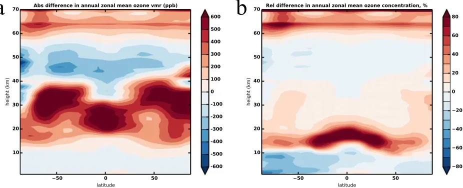
Hassler et al. 2008). Comparing the UKCA modeled ozone concentrations with those from the BDBP confirms that, on average in the tropics (108S–108N), the UKCA modeled ozone concentrations are around 16% higher than those observed.Figure 14shows that, while in absolute terms, the difference between the modeled and these observed ozone concentrations is greatest around 20–30 km, in rel-ative terms the difference is greatest in the tropical tropo-pause region (up to 80%). It is this that leads to such a large impact on the modeled tropical tropopause temperature.

The question of how to improve the simulated in-teractive ozone concentrations is a complex one. Using an identical chemistry scheme, with identical emissions, the GA4.0 model configuration produces a maximum ozone bias of around 40% in the tropical tropopause region (not shown), as compared to 80% in GA6.0 (Fig. 14b). This is possibly due to the different dynamical cores used in GA4.0 and GA6.0 (see references inTable 1) causing the vertical transport of ozone into and out of this region to be different. Thus, the interaction between the physical and composition components of an ESM is complex, and crucial to the performance of the ESM.

5. Discussion and conclusions

This paper has documented the effects of the dy-namical, radiative, and microphysical processes having

the largest impact on the tropical tropopause tempera-ture, and the value of water vapor concentrations on entry to the stratosphere, in the latest version of the Met Office Unified Model (MetUM).

The numerical accuracy of vertical advection across the tropopause, determined in the MetUM by the in-terpolation and conservation schemes used within the advection routine, is found to be particularly important. Within the interpolation scheme, it is found necessary to ensure that small-amplitude wavelike motions across the changes in the vertical gradients of potential tem-perature and humidity at the tropopause are treated so as to be essentially reversible, and that any spatial smoothing of water vapor concentrations in the upper troposphere inherent in the vertical interpolation is kept to a minimum. Applying a conservation scheme, such that mass integrals of potential temperature and water vapor are conserved during vertical advection, is also found to be essential. Improving the vertical advection in this way, the modeled tropical tropopause tempera-ture and lower-stratospheric water vapor concentrations are brought significantly closer to their observed values. Modifications to all processes discussed in this paper, with the exception of those to the model advection schemes, were found to have a detrimental impact on either the cold-point temperature bias or the lower-stratospheric water vapor bias. For some of the pro-cesses considered, such as the microphysical properties of ice particles (e.g., their particle size distribution and mass–diameter relationship), there exist observations under some atmospheric conditions (Field et al. 2007;

Cotton et al. 2013) that can be used to constrain the model parameterization. It is reasonable, in the absence

of other observations for those processes, to extrapolate these observations to the tropical tropopause region. Model improvements to the representation of radiative absorption, ice particle size distributions, and ice fall speeds (in the sense of moving closer to these extrapo-lated observations) will impact both the temperature and the water vapor concentrations in the tropical tro-popause region. The fact that these improvements were found to have a detrimental impact on the modeled cold-point temperature and lower-stratospheric water vapor concentrations (relative to GA6.0) is suggestive of the continuing presence of previously compensating errors, or of the fact that there are further improvements still required to these parameterizations.

Further sensitivity was found to convective and cirrus cloud processes. There are no observational constraints for the adaptive detrainment rate in the convection scheme (Derbyshire et al. 2011) or for the cirrus spreading rate in the cloud scheme. Therefore, while cloud heights are reasonably well observed, there remains significant flexi-bility for modification of parameters within the convection and cloud schemes to improve the simulation of well-constrained model fields, such as temperature. These schemes contribute significantly to the uncertainty in upper-tropospheric water vapor concentrations.

The importance of the vertical distribution of ice and water vapor in the TTL, and in particular a model’s representation of deep convection, cloud radiative, and ice-phase microphysical processes on its simulated TTL temperatures, is discussed also inEvan et al. (2013). The processes influencing tropical tropopause temperature and lower-stratospheric water vapor discussed in the current paper fall into three categories: dynamical processes (model advection), radiative processes (sensitive to water vapor and ice, cloud cover, and greenhouse gases), and microphysical processes that act as upper-tropospheric water vapor sources (tropical convection) and sinks (ice particles). How efficient the ice is as a sink of water vapor is dependent on the ice particle size distribution and fall speed. The ice crystal growth rate and sedimentation flux is itself sensitive to cirrus cloud fraction.

The impacts of all these processes on temperature, via the model advection and radiation schemes, can signifi-cantly alter the zonal-mean cold-point temperature at the tropical tropopause shown, for example, byGettelman et al. (2010)to be highly correlated to lower stratospheric water vapor concentrations. Furthermore, the impacts of these processes on upper-tropospheric water vapor con-centrations have a greater influence on lower-stratospheric water vapor concentrations in climate models than in the real world, because of the vertical transport of biases in upper-tropospheric water vapor concentrations nec-essarily included within the model vertical advection of

moisture. Thus, the uncertainty in upper-tropospheric water vapor concentrations arising in part from the model’s various parameterization schemes is particularly relevant to correctly modeling stratospheric water vapor concentrations. Of course, with sufficient vertical and temporal resolution, such vertical smoothing will be min-imized (C. Smith et al. 2015, unpublished manuscript).

Accurate modeling of stratospheric water vapor con-centrations is essential, as they directly influence surface climate, the tropospheric jet streams, and the evolution of stratospheric chemistry. If modeled interactively, the radiative impacts of greenhouse gases can further in-crease the uncertainty in stratospheric water vapor.

In general, the processes discussed in this work are found to have a minimal impact on temperatures and water vapor concentrations outside the tropopause re-gion (not shown). Of course, in addition to these pro-cesses, there are other processes impacting the tropical tropopause region. For example, the magnitude of gravity wave fluxes into the stratosphere is poorly con-strained and will influence the magnitude of the Brewer– Dobson circulation. This, in turn, is known to influence the cold-point temperature (Gettelman et al. 2010). However, in the MetUM this process was not found to have a significant impact on the temperature of the tropical tropopause or on stratospheric water vapor concentrations, and so has not been discussed in this work. Another process found to have negligible impact on tropical tropopause temperatures was the latent heat of vaporization of ice in this region. Also, the effect of cirrus clouds on the radiation budget, and therefore the cold-point temperature, can be influenced by the pres-ence of anthropogenic aerosols through aerosol indirect effects (Haywood and Boucher 2000; Sherwood 2002;

Gettelman et al. 2012), although these are only consid-ered via cirrus cloud amounts in this study.

The focus of this study has been mainly on annual-mean biases. In the MetUM it is found that annual-annual-mean biases in tropical tropopause temperature and strato-spheric water vapor are positive, but the biases in the magnitude of the seasonal cycle of these quantities are negative (i.e., the modeled annual cycle is too weak). Most of the processes discussed in this paper tend to increase or decrease both, which suggests that there may be other processes that are still missing from the model or that further improvement is required to those pro-cesses discussed. Therefore, improving both the annual-mean biases and the biases in the magnitude of the seasonal cycle is certainly a subject for further work.

one of these processes can produce a bias in the trop-ical tropopause region large enough to impact the simulated climate change, and accurate modeling of each process is therefore important for performing accurate climate simulations with that ESM. The tropical tropopause temperature bias and tropical lower-stratospheric water vapor concentrations provide a met-ric for simultaneously constraining both physical and Earth systems processes and their feedbacks. This study has used sensitivity experiments to understand the effects of individual processes, and it is hoped that the insight into these processes gained from this study will help other Earth system modeling groups to more accurately repre-sent both tropical tropopause temperatures and strato-spheric water vapor concentrations.

Acknowledgments.The authors thank Steve Derbyshire, Markus Gross, David Jackson, Adam Scaife, and Alison Stirling for useful discussions during the early stages of this work. The work of SCH, NB, FO’C, and KW was supported by the Joint DECC/Defra Met Office Had-ley Centre Climate Programme (GA01101). SCH and NB were supported by the European Community within the StratoClim project (Grant 603557). MW received funding by the Australian Government through the Australian Climate Change Science Programme. We acknowledge use of the MONSooN high performance computing system, a collaborative facility supplied under the Joint Weather and Climate Research Pro-gramme, a strategic partnership between the Met Of-fice and the Natural Environment Research Council. ERA-Interim data have been provided by the ECMWF Data Server. MERRA data have been have been pro-vided by the Global Modeling and Assimilation Office (GMAO) at NASA Goddard Space Flight Center through the NASA GES DISC online archive. The authors thank Greg Bodeker (Bodeker Scientific) and Birgit Hassler (NOAA) for providing the combined vertical ozone profile database. The authors acknowl-edge Sean Davis and Karen Rosenlof for permitting use of the SWOOSH dataset. The authors thank Mark Machin for producingFig. 1. This paper is U.K. Crown Copyright.

REFERENCES

Baran, A. J., P. Hill, K. Furtado, P. Field, and J. Manners, 2014: A coupled cloud physics–radiation parameterization of the bulk optical properties of cirrus and its impact on the Met Office Unified Model Global Atmosphere 5.0 configuration.J. Climate,

27,7725–7752, doi:10.1175/JCLI-D-13-00700.1.

Bodas-Salcedo, A., and Coauthors, 2011: COSP: Satellite simula-tion software for model assessment.Bull. Amer. Meteor. Soc.,

92,1023–1043, doi:10.1175/2011BAMS2856.1.

Bodeker Scientific, 2008: The Binary Data Base of Profiles, tier 1.4, version 1.1.0.6. Bodeker Scientific, accessed 10 February 2014. [Available online at http://www.bodekerscientific.com/data/ the-bdbp.]

Brown, A., S. Milton, M. Cullen, B. Golding, J. Mitchell, and A. Shelly, 2012: Unified modeling and prediction of weather and climate: A 25-year journey.Bull. Amer. Meteor. Soc.,93, 1865–1877, doi:10.1175/BAMS-D-12-00018.1.

Butchart, N., 2014: The Brewer–Dobson circulation.Rev. Geophys.,

52,157–184, doi:10.1002/2013RG000448.

Chepfer, H., S. Bony, D. Winker, M. Chiriaco, J.-L. Dufresne, and G. Sè_{ze, 2008: Use ofCALIPSOlidar observations to evaluate} the cloudiness simulated by a climate model.Geophys. Res. Lett.,35,L15704, doi:10.1029/2008GL034207.

Ciais, P., and Coauthors, 2013: Carbon and other bio-geochemical cycles. Climate Change 2013: The Physical Science Basis.T. F. Stocker et al., Eds., Cambridge Uni-versity Press, 465–570.

Cionni, I., and Coauthors, 2011: Ozone database in support of CMIP5 simulations: Results and corresponding radiative forcing.Atmos. Chem. Phys.,11,11 267–11 292, doi:10.5194/ acp-11-11267-2011.

Collins, M., S. F. B. Tett, and C. Cooper, 2001: The internal climate variability of HadCM3, a version of the Hadley Centre cou-pled model without flux adjustments.Climate Dyn.,17,61–81, doi:10.1007/s003820000094.

Cotton, R. J., and Coauthors, 2013: The effective density of small ice particles obtained from in situ aircraft observations of mid-latitude cirrus.Quart. J. Roy. Meteor. Soc.,139,1923–1934, doi:10.1002/qj.2058.

Cullen, M. J. P., 1993: The Unified Forecast/Climate Model.Meteor. Mag.,122,81–94.

Cusack, S., J. M. Edwards, and J. M. Crowther, 1999: Investigating

kdistribution methods for parameterizing gaseous absorption in the Hadley Centre Climate Model.J. Geophys. Res.,104 (D2), 2051–2057, doi:10.1029/1998JD200063.

Dee, D. P., and Coauthors, 2011: The ERA-Interim reanalysis: Configuration and performance of the data assimilation sys-tem.Quart. J. Roy. Meteor. Soc.,137,553–597, doi:10.1002/ qj.828.

Derbyshire, S. H., A. V. Maidens, S. F. Milton, R. A. Stratton, and M. R. Willett, 2011: Adaptive detrainment in a convective parametrization.Quart. J. Roy. Meteor. Soc.,137,1856–1871, doi:10.1002/qj.875.

Dessler, A. E., M. R. Schoeberl, T. Wang, S. M. Davis, K. H. Rosenlof, and J.-P. Vernier, 2014: Variations of strato-spheric water vapor over the past three decades.

J. Geophys. Res. Atmos.,119,12 588–12 598, doi:10.1002/ 2014JD021712.

Dinh, T., and S. Fueglistaler, 2014: Microphysical, radiative, and dynamical impacts of thin cirrus clouds on humidity in the tropical tropopause layer and lower stratosphere.Geophys. Res. Lett.,41,6949–6955, doi:10.1002/2014GL061289. ECMWF, 2011: ERA-Interim dataset (January 1979 to present).

ECMWF Data Server, accessed 20 October 2014. [Available online at http://apps.ecmwf.int/datasets/data/interim-full-moda/?levtype5pl.]

Edwards, J. M., and A. Slingo, 1996: Studies with a flexible new radiation code. I: Choosing a configuration for a large-scale model.Quart. J. Roy. Meteor. Soc.,122,689–719, doi:10.1002/ qj.49712253107.