The use of reflected Rayleigh waves to study rough contact interfaces

This is a repository copy of The use of reflected Rayleigh waves to study rough contact

interfaces.

White Rose Research Online URL for this paper:

http://eprints.whiterose.ac.uk/94608/

Version: Accepted Version

Article:

Ooi, E.S. and Dwyer-Joyce, R.S. (2015) The use of reflected Rayleigh waves to study

rough contact interfaces. Proceedings of the Institution of Mechanical Engineers, Part J:

Journal of Engineering Tribology. ISSN 1350-6501

https://doi.org/10.1177/1350650115600000

[email protected]

https://eprints.whiterose.ac.uk/

Reuse

Unless indicated otherwise, fulltext items are protected by copyright with all rights reserved. The copyright

exception in section 29 of the Copyright, Designs and Patents Act 1988 allows the making of a single copy

solely for the purpose of non-commercial research or private study within the limits of fair dealing. The

publisher or other rights-holder may allow further reproduction and re-use of this version - refer to the White

Rose Research Online record for this item. Where records identify the publisher as the copyright holder,

users can verify any specific terms of use on the publisher’s website.

Takedown

If you consider content in White Rose Research Online to be in breach of UK law, please notify us by

The use of reflected Rayleigh waves to study rough contact

interfaces

Eng S Ooi and R S Dwyer-Joyce

Leonardo Centre for Tribology and Surface Technology, Department of Mechanical Engineering, University of Sheffield, Sheffield, UK

Abstract: Ultrasonic reflectometry is commonly used in the field of tribology. Bulk waves that travel

through a component and are reflected from an interface can be used to measure parameters such as contact stress and lubricant film thickness. This paper presents the development of a novel ultrasonic technique using Rayleigh waves that propagate along the surface of a component. An analytical model is first proposed to explain the interaction of Rayleigh waves with a contact interface. When contact parameters change, so does the amplitude of the reflected Rayleigh wave. From the reflected waves, it is possible to simultaneously predict both normal and tangential interface stiffness. Experiments have been conducted to show how the reflected waves change as cyclic loading is applied and the

roughness of the contact interface varied. Results have shown there is good agreement between experimental data and analytical predictions. Potential application of this study includes the remote monitoring of sealing components such as o-rings or radial lip seals.

Keywords: Rayleigh waves, ultrasonic reflection, Hertzian contact, contact stiffness, rough surface

contact

1 Introduction

One approach for the measurement of contact parameters is by recording the proportion of an ultrasonic pulse that is reflected from the interface. Several authors have used ultrasonic bulk waves in this way. Kendall & Tabor [1] used ultrasonic waves to study the real contact area between two bodies. Pialucha and Cawley [2] used ultrasound to detect and quantify the thickness of a thin layer sandwiched between two much thicker media. Contact stiffness measurements using both longitudinal and shear bulk waves were made in separate studies by Krolikowski and Szczepek [3] and Biwa and co-workers [4]. Ultrasound has also been shown to measure contacts and oil films in actual

engineering components such as bearings [5], mechanical seals [6], railway contacts [7] and interference fits [8].

There are however, several limitations to the use of bulk (i.e. travelling through the material and usually normal to the contact interface) ultrasonic waves. If the material in which the pulse is travelling is highly attenuative e.g. elastomeric seals and rubber gaskets, little or no reflection is obtained. Also, many tribological components have complex geometries that introduce multiple interfaces or discontinuities through which the pulse would have to pass before reaching the interface of interest. These intermediate interfaces cause unwanted reflections which reduce the overall energy content of the signal. Coupled with background noise, the signal strength can be severely attenuated.

To overcome these issues, the use of Rayleigh waves to analyse tribological interfaces is proposed. One of the main advantages of using Rayleigh waves is that instead of travelling through the bulk of the material, they travel along the surface. When there is a change to the topography of the Rayleigh wave path, such as that caused by an interface, the waves will be scattered. This paper details the development of an analytical model that describes the interaction of Rayleigh waves with a contact interface. This model is then compared with experimental results where the reflections of a Rayleigh wave from a series of rough contact interfaces have been measured.

the configuration involved makes it more practical to use Rayleigh waves instead of conventional bulk waves.

2 Background

A Rayleigh wave is a type of wave mode that propagates along the surface of a half space. It is a combination of both the longitudinal and transverse waves propagating simultaneously and decaying exponentially into the medium. Reflections are caused by sudden changes in the wave path. These can be caused by changes in the topography of the medium (e.g. a crack, a raised profile) or changes at the surface (e.g. a drop of liquid or a solid body coming into contact). Rayleigh wave reflection has been widely used in the area of flaw detection [9,10] for near surface defects and cracks.

Reflections due to changes in the topography of the medium

Early work by Viktorov [9] showed how Rayleigh waves are reflected at the edge of a specimen with varying angles (Fig.1a). Graczykowski [11] developed finite element models to study how surface waves were reflected from three different geometries (Fig.1c,d,e). The results show that the maximum reflection coefficients in these cases were around the region of 0.2 – 0.25. These values were affected by the dimensions of the steps and grooves. The reflection from the edge of a quarter space (Fig.1b) by Gautesen [12], was studied numerically for both reflected and transmitted waves, the results of which are used later in the present study.

Fig.1 Sources of Rayleigh wave reflection

Reflections due to changes at the surface of the medium

Reflections of Rayleigh waves also arise due to changes in the bordering medium such as a liquid or a body in contact with the surface. Work on reflected surface waves from a liquid loaded surface have been conducted by Newton et al [13] and McHale et al [14]. In their work, a strip of viscous fluid (Fig.1g) was introduced directly into the path of a travelling surface wave. Resonances were observed as the liquid spreads across the surface. Experiments conducted by Rudy [15] have proved the existence of reflected Rayleigh waves from a loaded surface by bouncing the signals off a piston ring. The waves were sent down the cylinder and echoes recorded from the piston ring to determine the location of the contact. Possibly the most common Rayleigh reflection phenomenon is that occurring at mechanical gratings (Fig.1f) which can be found in most surface acoustic wave (SAW) devices used in telecommunications. The reflection from mechanical gratings were studied using either the perturbation method or the variational approach [16].

from along the positive x-axis. As the spring vibrates, some of the vibrations are transferred back to the base and returns to the source as reflected waves. The model was developed with the purpose of examining reflecting elements in SAW devices instead of a classic tribological interface. In this paper, a new model is proposed to explain the interaction of Rayleigh waves with a contact interface.

3 Response of Rayleigh wave from an interface

The material through which the Rayleigh wave travels is modelled as an elastic isotropic half-space. Fig.2 shows a cylindrical specimen pressed, with a normal load P, onto the half-space to create a line contact of length, and width 2a. The contact is modelled as a spring with both normal and tangential stiffness, denoted as and as shown.

Fig.2 Model of the Contact Interface

A Rayleigh wave is a combination of both a longitudinal component, UI and a transverse component,

WI. In Fig.2, the two components are shown separately. The displacement as a function of time, t and

distance from the origin, x are given by [9]:

cos⁡ (1)

⁡ sin (2)

Where B is an amplitude coefficient, and is the wave frequency. kr, kl, and kt are the wavenumbers

of the Rayleigh, longitudinal, and transverse waves respectively, and:

As both WI and UI travels along the positive x direction, they will eventually impinge on the interfacial

springs. WI causes excitation of the spring in the y-direction while UI causes excitation of the spring in

the x-direction. The development of the equations that follow will be broken down into two parts; displacements corresponding to these two axes.

3.1 Displacements caused by incident wave components WI and UI

Excitation of the spring by WI causes the spring to oscillate vertically (Fig.3a). The oscillating motion

Rayleigh waves in the half space. The wave field generated by the periodic force caused by the spring on the surface of the elastic half-space has been solved by Lamb [18]. Of interest in this study is the reflected Rayleigh wave. Expressions for vertical and horizontal displacements of a reflected Rayleigh wave due to WI are:

(3)

(4)

Where the periodic force due to vertical spring excitation, G is the shear modulus and are constants that are functions of the half-space Poisson’s ratio

Fig.3 Reaction of the interface due to vertical & horizontal excitations

In the same manner, the horizontal component of the incident Rayleigh wave, UI also generates

reflected Rayleigh waves (Fig.3b), the expressions of which have also been derived by Lamb [18]. As before, the expressions for vertical and horizontal displacements are:

(5)

(6)

Where is the periodic force due to horizontal spring excitation and are constants that are functions of the half-space Poisson’s ratio.

Fig.4 Values of constants and⁡ variation with Poisson’s ratio, 3.2 Deriving reflection coefficient

The reflection coefficient in the x-direction, Rx is defined as the total reflected displacement in the

x-direction divided by the incident displacement in the x-x-direction and likewise Ry in the y-direction.

Thus;

⁡ ⁡ (7)

⁡

(8)

Equations (7) and (8) can be simplified by recognizing that the stiffness of an interface in the normal and tangential directions, K and K respectively, are given by:

⁡ (9)

⁡ (10)

Combining (9) and (10) with equations (7) and (8) gives:

(11)

(12)

The total reflection coefficient is then:

3.3 Interface stiffness

Fig.5 shows how normal stiffness, changes as the interface is normally loaded (the case for tangential stiffness, is analogous). Initially, at zero load the normal stiffness, – the gradient of the load-displacement curve is zero; this occurs at the origin. increases non linearly as load is applied. At an applied load of P, the equilibrium point is (y,P), as shown in Fig.5. When vertical components of the incident Rayleigh wave, WI impinges on the interface, it causes the spring to

oscillate about this equilibrium. This results in a periodic change between a relaxation and a further compression of the spring as shown in Fig.5. In practice, WI is a very small value so it is reasonable to

define the normal stiffness as:

Gradient⁡at⁡ ⁡ Gradient⁡at⁡ (14)

Fig.5 Graphical representation of changes in normal stiffness

The changes in tangential stiffness are analogous to the normal stiffness so:

(15)

(16)

(17)

Where K-a and K-b are the asperity and bulk stiffness components for normal stiffness. Likewise K-a

and K-b are the asperity and bulk stiffness components for tangential stiffness.

Fig.6 Multi-scale stiffness in a line contact

Stiffness Due to Asperity Interactions

For a line contact, the stiffness due to asperity interaction is derived from works by Lo [20] and Gelinck and Schipper [21]. The basis of their work assumes that the asperities lie along a profile that is a function of the x-axis due to the curvature involved. In general, the solution to the problem is difficult and requires involved algorithms (e.g. Gelinck and Schipper uses multigrid algorithms).

However, the problem can be greatly simplified by assuming that the cylinder remains rigid when pressed onto the surface. This assumption is approximately true when the surfaces are rough as the asperities are considered to deform readily as opposed to the bulk of the cylinder. Doing so yields stiffness of the form (for a Gaussian distribution of asperities)

e ⁡ ∞

∞ (18)

Where is the asperity density, is the radius of the asperity tip, h is the separation between the two surfaces, is the combined RMS roughness of the two surfaces ( and E’ is the

combined youngs modulus . and are the Poissons ratio and elastic modulus of the half space and cylinder respectively. The quantities , and can be estimated from profilometer measurements of a particular surface while h can be obtained by satisfying the force balance equation [22] given by equation (19)as

⁡ ⁡ ⁡ (19)

Where p(z,x) is the distributed load at the contact interface given as [20,21]

exp⁡ ⁡

(20)

We further assume that the tangential stiffness is proportional to the normal stiffness. This is inherently true for a single asperity contact as shown by Mindlin [23]. In general, for rough surfaces in contact the stiffness ratio has the form:

(21)

Where A is a constant that has differing values depending on the distribution and shape of asperity peaks assumed. A summary for the values of A is given by Gonzalez et al [24] where, for a Poissons ratio = 0.3, 0.7<A<2.

Stiffness Due to Bulk Deformation

The case of a smooth cylinder pressed onto a rigid flat has been analytically studied by Puttock and Thwaite [25]. Their results for the surface deformation can be extended to give an expression for the normal stiffness:

(22)

For identical materials in contact equation (22) reduces to:

ln⁡

(23)

Although some studies on the tangential loading applied onto a line contact have been done, mathematical difficulties prevent the evaluation of a closed form solution. Experimental results of stiffness ratios [3,4,24] strongly suggest that the normal and tangential stiffness have an almost constant proportionality between them. Therefore for simplicity, we assume that the stiffness ratio due to bulk deformation is a constant and follows the definition given by equation (21), and so:

(24)

4 Analytical prediction of Rayleigh wave response from an interface

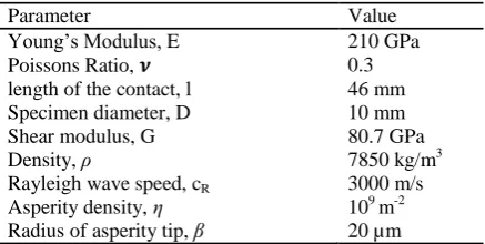
Table 1 Properties of the contact interface

Parameter Value

Young’s Modulus, E 210 GPa

Poissons Ratio, 0.3 length of the contact, l 46 mm Specimen diameter, D 10 mm Shear modulus, G 80.7 GPa

Density, 7850 kg/m3

Rayleigh wave speed, cR 3000 m/s

Asperity density, 109 _m-2

To illustrate the interplay between the contact parameters, calculations were performed on a sample case of a steel-steel contact. Calculations were performed for A=0.7 with varying combined roughness, . Table 1 gives the values of the other required parameters used in the calculations.

Given the sample parameters, h was calculated by satisfying the force balance equation at the contact

[22] and was approximated as ⁡ ln .

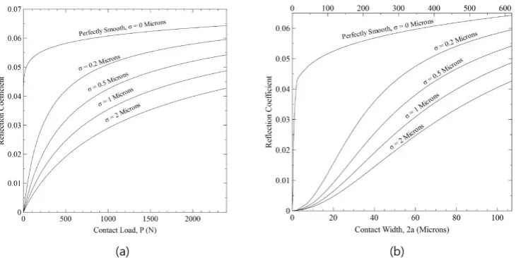
The results for stiffness and are plotted in Fig.8. As and are in direct proportion, the curves are identical but with a different y-axis scale. The ordinate is expressed both as the applied contact load, Fig. 8a and the resulting Hertzian contact width and maximum pressure, Fig. 8b. As the contact load is increased, the interface becomes stiffer (i.e. the rough contact becomes more complete and an increase in load causes little approach of the surfaces). Likewise, a reduction in the roughness increases the reflection coefficient.

Fig. 7 Analytical plots of K and K as they vary with (a) contact load, P and (b) contact width 2a.

Fig.8 Analytical plots of Reflection Coefficient as it varies with (a) contact load, P and (b) contact

Fig.8shows the reflection coefficient obtained by applying equations (11), (12), and (13) to the data of Fig. 7. The stiffer the contact the greater the reflection of the Rayleigh wave. Also shown is the upper limit of reflection coefficient where the interface is assumed to be perfectly smooth. This gives an indication of the maximum value of reflection coefficient that can be obtained from a given case.

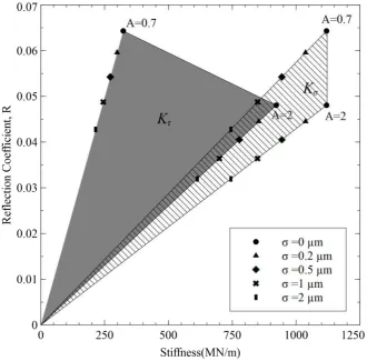
Combining (11), (12) and (13) with (21) and (24), the following expressions are obtained

(25)

(26)

Thus reflection coefficient is directly proportional to both Kj and Kk. (25) and (26) are plotted in Fig. 9 and it can be seen that plots of R against Kj and Kk appear as straight lines through the origin. The

plotted data points represent the endpoints (P=2400N) for the line that is traced by each data set for different .

To demonstrate the effect of A, both the upper and lower limit for A has been plotted. Based on (24), increasing A for a Poisson’s ratio of 0.3 has the effect of decreasing the relative difference between

and i.e. the stiffness ratio approaches unity. This is reflected in Fig. 9 where the lines of and approaches each other as A is increased. For intermediate values of A, the plots for and will fall in their respective shaded regions.

Thus, if the stiffness ratio for a contact interface is known; this allows for a convenient way of predicting contact stiffness by virtue of reflection coefficient from Rayleigh waves alone, without having to first characterise the nature of the surfaces in contact.

5 Experimental apparatus and instrumentation

5.1 Model Contact and Loading Apparatus

Fig.10 Physical layout of the experiment

The experimental contact (shown in Fig.10) consisted of a steel rod (46 mm contact length and 10 mm in diameter) pressed against a steel block in a servo-hydraulic tension-compression machine operating in load control. This allows a consistent loading-unloading cycle to be applied on to the specimen. The maximum load applied was 2.4 kN which corresponded to a maximum contact pressure of 621 MPa and a contact width of 107 µm.

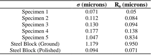
Table 2 Roughness parameters

j

(microns)

R

(microns)

Specimen 1 0.071 0.05 Specimen 2 0.112 0.084 Specimen 3 0.130 0.094 Specimen 4 0.177 0.138 Specimen 5 1.047 0.834 Steel Block (Ground) 1.179 0.950 Steel Block (Polished) 0.094 0.071

5.2 Ultrasonic Instrumentation

To generate the Rayleigh wave, the wedge method was used whereby the transducer is coupled to the sample using a Perspex wedge as shown in Fig.10. The angle, at which the Rayleigh wave was generated is called the Rayleigh angle. It is dependent on the longitudinal wave speeds in both the wedge and the steel block. For a Perspex – steel combination, this is approximately 65o. Coupling the wedge with the block is achieved using a thin layer of viscous oil. The wedge was fitted with a longitudinal wave transducer (Panametrics Model NDT A403S) with a centre frequency of 2.25 MHz which operates in pulse-echo mode. The transducer itself generates regular longitudinal waves, as the longitudinal waves hit the interface at the Rayleigh angle, the longitudinal waves are transformed into Rayleigh waves which then travel along the surface of the steel block.

An integrated ultrasonic data acquisition system was used both to drive the transducer and to record the incoming reflections. Fig.11 shows the main features of the ultrasonic system used in the experiment. Transducer pulsing parameters and amplification of the received signals were controlled through an Ultrasonic Pulser Receiver (UPR) card using a program written in the LabVIEW environment. The integrated system was controlled by a PC fitted with a high speed 8 channel data acquisition card (DAQ) which captures and stores the required data for further post processing.

Fig.11 Schematic of ultrasonic system

The transducer performed in pulse-echo mode whereby signals were transmitted and received using the same transducer. The received signals from the transducer (i.e. the reflected Rayleigh waves) were digitized and displayed in real time on a virtual oscilloscope. The UPR was set to pulse at 2.2 MHz centre frequency at 100 volts. As the load was applied, the ultrasonic system continuously recorded the reflected pulse at a rate of 160 pulses per second. This provides a full picture of how the amplitude of the reflected pulse evolves during the loading cycle.

5.3 Signal Processing

The first step was to record a reference time domain signal. This was done by sending a wave across the surface of the steel block and recording all nominal reflections i.e. reflections due to the input pulse and those from the boundaries of the steel block, as shown in Fig.12a. The nominal reflections A, B and C occur at the refraction interface and substrate edges as indicated in the insert diagram. The specimens were then loaded and the signal recorded. As shown in Fig.12b, the appearance of a reflected pulse, D can be observed.

Transducer DAQ Systems

UPR (Ultrasonic Pulser Receiver) Card Rayleigh Waves

Transmit-Receive operation using the same

Signals sent to PC to be processed

Fig.12 Identifying reflected pulse in the time domain (a) without specimen and (b) with specimen

Pulse D was extracted from the waveform. To obtain the reflection coefficient this pulse must be divided by the amplitude of the incident pulse. The amplitudes for the incident pulse could either be measured directly through the use of an identical transducer or by estimating it using reflections from a known geometry. In this study, the latter option has been used. Fig.13a shows how reflected and transmitted Rayleigh waves are produced as a result of an incident Rayleigh wave striking the edge of a quarter space, a geometry that is identical to that creating pulse B in Fig.12. Through numerical methods, the reflection and transmission coefficients for a Rayleigh wave striking the edge of a quarter space was calculated by Gautesen [12], the results of which are summarized in Fig.13b.

Fig.13 Rayleigh wave reflection from an elastic quarter space [12]

A collection of reflected pulses (i.e. pulse D), taken at four discrete load steps of 500 N up to 2000 N is shown in the time domain in Fig.14 after a bandpass filter has been applied to remove noise.

Fig.14 Time domain pulses reflected from the contact at various applied loads.

To get a measure of the changes in amplitude, the time domain data was converted into the frequency domain by using the Fast Fourier Transform (FFT) algorithm. The FFT was performed for each reflected pulse and the results are shown in Fig.15. These pulses were then divided by the incident pulse to yield reflection coefficient (Fig.16) at a bandwidth of -2.5 dB or 75% of the peak amplitude of the reference pulse which resulted in a frequency range between 1.9 MHz to 2.4 MHz. Outside this bandwidth, the data become increasingly noisy and was thus discarded. In the actual test, the time domain waveform was captured at a rate of 160 times per second to obtain a continuous change in reflected waves as load was increased.

The reflection coefficient can easily be converted to and using the gradients of the lines in Fig. 9 provided A is known. To illustrate, the conversion to stiffness in Fig.16 was done for A=0.7. As would be expected, the measured reflection coefficient and hence stiffness components and are largely unaffected by the frequency. The slight waviness is attributed to electrical and background noise from the measuring apparatus.

Fig.16 Reflection coefficient and stiffness components at -2.5dB bandwidth.

6 Results and discussions

A series of three controlled load cycles were applied. The specimens were not unloaded to zero load, but rather, care was taken to ensure that there was a small residual load (≈ 5 N) to ensure that the surfaces continue to stay in contact. This prevented relative movement of the surfaces, allowing the load to always be applied on the same asperity contacts at each subsequent cycle.

Fig.17a shows the reflection recorded during these three loading cycles for a rough and a smooth contact pair plotted against the equivalent Hertzian maximum pressure. The rough and smooth contact pairs were generated by pressing specimen 1 against the ground and polished block respectively.

Fig.17 (a) Reflection cofficient recorded during three loading cycles for two different roughness

contact pairs. (b) With analytical curves overlaid

For the smooth case subsequent loading cycles are largely elastic as shakedown has occurred. In contrast, subsequent cycles for the rougher contact exhibit a repeating hysteresis loop. This suggests a

“repeatable irreversibility” caused by an increase in roughness of the interface. Similar phenomenon were observed in early work on ultrasonic bulk waves [24,26,27] where this hysteresis was attributed to irreversible adhesion at the interface.

Also shown in Fig.17b are the analytical predictions calculated for the limits of A=0.7 to A=2 calculated for both contact pairs. The radius of the asperity tip, and asperity density, required in generating the analytical curves were obtained from the measured profiles of the contact. For the case

where is 0.118 µm, and were estimated to be 47µm and 7×1010 m-2 respectively. When is 1.181 µm, and takes the value of 10.34 µm and 0.65 × 109 m-2.

The agreement between predicted and analytical results is well within an order of magnitude of each other, with a better match obtained at the limits of A=0.7. The equivalent stiffness corresponding to A=0.7 are shown on a separate axis.

One source of error arises from the fact that in calculating the asperity stiffness, the analytical model assumes elastic deformation of the asperities. It is clear from the observed hysteresis loops that plastic deformation of the asperities takes places, causing deviations from the analytical model. The plastic deformation is less pronounced in the case of a smooth contact, hence the match is better in this case (at A=0.7).

Relaxation of full elastic assumption may allow the prediction of plastic effects, but at the cost of greater complexity in the analytical model. This can be done by using plastic contact models and incorporating them into the definition of asperity stiffness in section 3.3. An example of a line contact model that considers plasticity has been developed by Behesti and Khonsari [22].

The analytical model derived in the work here describes the response of Rayleigh waves as it interacts with a contact interface and is dependent on proper prediction of contact stiffness. For a smooth surface, the stiffness models can be readily determined from contact mechanics since they represent idealized cases. However, stiffness models for cases where the surfaces are rough are in general statistical in nature and are never exact since any two surfaces can never truly be identical on the micro-scale. This is compounded by the fact that the idealizations made in some of the models are far removed from the actual cases but are nonetheless still widely used due to their simplistic nature. Thus the accuracy of the model can only be as accurate as the stiffness models themselves.

Fig.18 Reflection coeficient recorded during the third loading cycle for a range of different roughness

pairs.

Fig.18 shows results for the third loading cycle for a range of rough contacts, achieved by using different combinations of the specimens in Table 2 pressed against the polished steel block. Again, the rougher specimens exhibit more hysteresis. In some cases, where the specimens were not perfectly straight along their axis, the contact area at low loads decreased due to the added curvature. This resulted in a lower reflection coefficient while flattening of the specimens takes place, as shown in Fig.18.

Although the study here was focused on a line contact, the analytical model was developed such that contact of different configurations can be studied; as long as the contact width is several orders of magnitudes smaller than the wavelength of the Rayleigh waves to maintain the assumption that the contact can be viewed as a discrete interface (c.f. section 3.1). For example, the case for a flat contact can be studied if expressions for flat contacts were utilized in the calculation of the stiffnesses.

7 Summary and Conclusions

An analytical model that predicts the interaction of Rayleigh waves with a line contact has been developed. The model describes the interface as a series of springs with the stiffness controlling the amount of wave being reflected from the interface. It is shown from the analytical model that it is possible to simultaneously predict both normal and tangential stiffness provided that the stiffness ratio of the contact is known.

Experiments were conducted with variable roughness components undergoing repeated normal loading. Hysteresis loops were observed with the size of the loops increasing as roughness increases. It is observed that increase in roughness reduces the reflection coefficient of the Rayleigh waves. Overall, the analytical model agreed well with experimental results at both smooth and rough contact interfaces.

References

1. Kendall.K, Tabor.D. An Ultrasonic Study of the Area of Contact Between Stationary and Sliding Surfaces. Proceedings of the Royal Society A. 1971;323:321–40.

2. Pialucha T, Cawley P. The detection of thin embedded layers using normal incidence ultrasound. Ultrasonics. 1994;32(6):431–40.

3. Królikowski J, Szczepek J. Assessment of tangential and normal stiffness of contact between rough surfaces using ultrasonic method. Wear. 1993;160(2):253–8.

4. Biwa S, Suzuki A, Ohno N. Evaluation of interface wave velocity, reflection coefficients and interfacial stiffnesses of contacting surfaces. Ultrasonics. 2005;43(6):495–502.

5. Dwyer-Joyce RS, Harper P, Drinkwater BW. A method for the measurement of hydrodynamic oil films using ultrasonic reflection. Tribology Letters. 2004;17(2):337–48.

6. Reddyhoff T, Dwyer-Joyce RS, Harper P. A new approach for the measurement of film thickness in liquid face seals. Tribology Transactions. 2008;51(2):140–9.

7. Marshall MB, Lewis R, Dwyer-Joyce RS, Olofsson U, Björklund S. Experimental

characterization of wheel-rail contact patch evolution. Journal of Tribology. 2006;128(3):493– 504.

8. Lewis R, Marshall MB, Dwyer-Joyce RS. Measurement of interface pressure in interference fits. Proceedings of the Institution of Mechanical Engineers, Part C: Journal of Mechanical Engineering Science. 2005;219(2):127–39.

9. Viktorov IA. Rayleigh and Lamb Waves; Physical Theory and Applications. New York: Plenum P; 1967.

10. Zachary LW. Quantitative use of Rayleigh waves to locate and size subsurface holes. Journal of Nondestructive Evaluation. 1982;3(1):55–63.

11. Graczykowski B. The reflection of Rayleigh surface waves from single steps and grooves. Journal of Applied Physics. 2012;112(10).

12. Gautesen AK. Scattering of a Rayleigh wave by an elastic quarter space - Revisited. Wave Motion. 2002;35(1):91–8.

13. Newton MI, McHale G, Banerjee MK. Reflection of surface acoustic waves by localized wetting liquids. Applied Physics Letters. 1997;71(26):3785–6.

15. Rudy T. An Ultrasonic Method of Measuring Piston Ring Bore Contact Patterns. SAE Technical Paper. Detroit; 1967. p. 1–8.

16. Robinson H, Hahn Y, Gau JN. A comprehensive analysis of surface acoustic wave reflections. Journal of Applied Physics. 1989;65(12):4573–86.

17. Plesskii VP, Simonyan A V. Reflection of Rayleigh waves from a resonant element. Akusticheskii Zurnal. 1991;37(1):162–6.

18. Lamb H. On the Propagation of Tremors over the Surface of an Elastic Solid. Philosophical Transactions of The Royal Society A. 1904;203:1–42.

19. Johnson KL. Contact Mechanics. 1st ed. Cambridge: Press Syndicate; 1985.

20. Lo CC. Elastic contact of rough cylinders. International Journal of Mechanical Sciences. 1969;11(1):105–6,IN7–8,107–15.

21. Gelinck ERM, Schipper DJ. Deformation of rough line contacts. Journal of Tribology. 1999;121(3):449–54.

22. Beheshti A, Khonsari MM. Asperity micro-contact models as applied to the deformation of rough line contact. Tribology International. 2012;52:61–74.

23. Mindlin RD. Compliance of elastic bodies in contact. Journal of Applied Mechanics. 1949;16:259–68.

24. Gonzalez-Valadez M, Baltazar A, Dwyer-Joyce RS. Study of interfacial stiffness ratio of a rough surface in contact using a spring model. Wear. 2010;268(2-3):373–9.

25. Puttock MJ, Thwaite EG. Elastic Compression of Spheres and Cylinders at Point and Line Contact. National Standards Laboratory Technical Paper. 1969;(25):15.

26. Drinkwater BW, Dwyer-Joyce RS, Cawley P. A study of the interaction between ultrasound and a partially contacting solid-solid interface. Proceedings of the Royal Society A: Mathematical, Physical and Engineering Sciences. 1996;452(1955):2613–28.

27. Dwyer-Joyce RS, Drinkwater BW, Quinn AM. The use of ultrasound in the investigation of rough surface interfaces. Journal of Tribology. 2001;123(1):8–16.