Nonlinear modal analysis using pattern recognition

White Rose Research Online URL for this paper:

http://eprints.whiterose.ac.uk/80985/

Version: Published Version

Proceedings Paper:

Dervilis, N., Wagg, D.J., Green, P.L. et al. (1 more author) (2014) Nonlinear modal analysis

using pattern recognition. In: Proceedings of ISMA2014. ISMA2014, 15-17 September

2014, KU Leuven. , 3017 - 3027.

[email protected] https://eprints.whiterose.ac.uk/ Reuse

Unless indicated otherwise, fulltext items are protected by copyright with all rights reserved. The copyright exception in section 29 of the Copyright, Designs and Patents Act 1988 allows the making of a single copy solely for the purpose of non-commercial research or private study within the limits of fair dealing. The publisher or other rights-holder may allow further reproduction and re-use of this version - refer to the White Rose Research Online record for this item. Where records identify the publisher as the copyright holder, users can verify any specific terms of use on the publisher’s website.

Takedown

If you consider content in White Rose Research Online to be in breach of UK law, please notify us by

N.Dervilis1, D.J.Wagg1, P.L.Green1, K.Worden1 1

Dynamics Research Group, Department of Mechanical Engineering, University of Sheffield, Mappin Street, Sheffield, S1 3JD, England. e-mail:[email protected]

Abstract

The main objective of nonlinear modal analysis is to formulate a mathematical model of a nonlinear dynamical structure based on observations of input/output data from the dynamical system. Most theories regarding structural modal analysis are centred on the linear modal analysis which has proved to now to be the method of choice for the analysis of linear dynamic structures. However, for the majority of other structures, where the effect of nonlinearity becomes significant, then nonlinear modal analysis is a necessity. The objective of the current paper is to demonstrate a machine learning approach to output-only nonlinear modal decomposition using kernel independent component analysis and locally linear embedding analysis. The key element is to demonstrate a pattern recognition approach which exploits the idea of independence of principal components by learning the nonlinear manifold between the variables.

1

Introduction

The machine learning methods that are introduced in this paper aim to address the problem of validity that surrounds the modal analysis of nonlinear structures. Modal analysis is an important tool in structural dynamics as it is used to understand the dynamical characteristics of the structure. Many methods have been proposed in recent years regarding nonlinear analysis, such as nonlinear normal modes or the method of normal forms [1, 2, 3, 4, 5, 6, 7, 8, 9].

In this work a different approach is investigated through the usage of unsupervised pattern recognition techniques such as kernel independent component analysis (KICA) and locally linear embedding manifold learning (LLE). These methods serve two purposes, a reduction in the dimensionality by mapping the data from high-dimensional spaces to lower-dimensional spaces and a revealing of the hidden features of the data by learning the structure of the nonlinear manifold between the variables of interest. Of course this dimensionality reduction is accompanied by loss of some information; therefore, the goal in dimensionality reduction should be to preserve as much relevant information as possible.

The goal of these methods is one: to create uncorrelated variables but retaining the maximum possible variance of the original observations. The effect of structural nonlinearity on linear modal analysis is critical. Specifically, decoupling of the system into SDOF systems is lost and in turn superposition is lost. It is of critical importance to mention that these clever and advanced unsupervised algorithms can work with output-only data and can play a significant role in the model updating of nonlinear systems by giving crucial insight into the dynamical behaviour of the system.

The layout of the paper is as follows. Section 2 covers the main features of linear modal analysis using linear decoupling methods such as principal component analysis, while section 3 discusses an alternative approach of independent component analysis (ICA). Section 4 gives an example of nonlinear modal analysis based on the unsupervised learning techniques that are mentioned in sections 2 and 3. Section 5 discusses how the

previous approaches break down for multi-degrees-of-freedom systems with high nonlinearity and a new approach based on measured data such as locally linear embedding method is needed. The paper finishes with some overall conclusion and future work.

2

Principal component analysis

Principal Component Analysis takes a multivariate data set and maps it onto a new set of variables called “principal components”, which are linear combinations of the old variables. The first principal component will account for the highest amount of the variance in the data set and the second principal component will account for the second highest variance in the data set independent of the first, and so on. The importance of the method arises from the fact that, in terms of mean-squared-error of reconstruction, it is the optimal linear tool for compressing data of high dimension into data of lower dimension. The unknown parameters of the transformation can be computed directly from the raw data set and, once all parameters are derived, compression and decompression are small operations based on matrix algebra [10, 11, 12]. One has,

[X] = [K][Y] (1)

Where[Y]represents the original input data with sizep×n, withpnumber of variables andnthe number of data sets,[X]is the scores matrix of reduced dimensionq×nwhereq < pcontains the tranformed varriables and[K]is called the loading matrix. The columns of[K]are the eigenvectors corresponding to the largest eigenvalues of the covariance matrix of[Y]. The covariance matrix is equal to:

[S] =Eh {Y} − {Y¯}

{Y} − {Y¯}Ti

(2)

whereEis the expectation operator andY¯ is the mean value.

The original data reconstruction is performed by the inverse of equation (1):

[ ˆY] = [K]T[X] (3)

The information loss of the mapping procedure is calculated in the reconstruction error matrix:

[E] = [Y]−[ ˆY] (4)

For further information on PCA, readers are referred to any text book on multivariate analysis (examples being references [10, 11]).

3

Kernel independent component analysis

Independent component analysis (ICA) is a tool that recovers a latent random vector{x} = (x1, ..., xm)

from measurements ofmunknown linear functions of that vector. The components of{x}are required to be mutually independent. As a result an observation{y}= (y1, ..., ym)is modelled as [13, 14, 15]:

{y}= [A]{x} (5)

where[A]is anm×mmatrix of parameters.

If[W] = [A]−1

{xˆ}= [W]{y} (6)

It can be shown [13, 14, 15] that minimising the mutual information between the components of (6) is essentially a contrast function minimisation.

Contrast functions are statistical functions that are capable of separating or extracting independent components from a data mixture [15]. If a contrast function is derived by theF-correlation statistics, it can be defined as the maximum correlation between the tested random variablesf1 andfm[15] and can be written as:

pf = max

f1_{,f m}∈fcorr(f1(x1), fm(xm)) = maxf1_{,f m}∈f

cov(f1(x1), fm(xm))

(varf1(x1))12(varf_m(x_m)) 1 2

(7)

for eachi...m, of estimated source vectors such as{x}= (x1, ..., xm). This contrast function is equal to zero

only if the variables are independent.

Different methods have been introduced in the literature regarding ICA that make use of different nonlinear contrast functions [13, 14, 15]. The nonlinear ICA method that is used in this study is kernel independent component analysis (KICA) which makes use of the “kernel trick” which is an algorithm that uses a multiple nonlinear functions but through an entire function space of a family of candidate nonlinearities. The “kernel trick” is basically forcing the functions to work in a reproducing kernel Hilbert space.

Given the nature of the current paper a full description of the complicated algorithm is not possible but for further information on ICA and Kernel ICA, readers are referred to [13, 14, 15].

Briefly the general outline of algorithm is as follows:

If one assumes[y] = ({y1}, ...,{ym})of data vectors and the parameter matrix[W]of equation (6), and set {x}= [W]{y}then one can derive a set of estimated source vectors such as[x] = ({x1}, ...,{xm}). Them

components of these vectors lead to a set ofmcentered kernel Gram matrices,[K1], ...,[Km].

Briefly, a Gram matrix can be generally defined as,Kij =K(xi, xj), which is positive semidefinite Kernel

matrix [15]. This kernel[K]matrix is accompanied by a mapping of a functionΦto anF-distribution such as:

K(x, y) =hΦ(x),Φ(y)i (8)

This kernel can be then used to compute the inner product in theF-distribution space. This is often called the

kernel trick. These kernel matrices can then be used in order to define a contrast function [15]:

C(W) = ˆIpf([K1], ...,[Km]) (9)

whereIˆpf is a contrast function given by:

ˆ

Ipf =−

1 2log

1− max

f1_{,f m}∈fcorr(f1(x1), fm(xm))

(10)

This valid contrast function is derived byF-correlation statistics and is defined as the maximum correlation between the tested random variablesf1andfm. [15].

is that while PCA works with a single random vector and maximises the variance of projections of the observations, CCA works with a set ofmrandom vectors by maximising the correlation between sets of projections [15]. One needs to remember that PCA solves an eigenvector problem, CCA solves a generalized eigenvector problem.

Another contrast function which can be defined is via the kernel generalised variance (KGV) algorithm which suggests defining a corresponding quantity for kernelized canonical correlation analysis [15]. For further information readers are referred to [15].

The basic concept that one has to remember is that ICA can remove correlations and higher order dependences between the variables compared to PCA (which can only go up to second order statistics).

4

An example

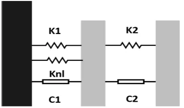
The system of interest will be a nonlinear two-DOF lumped parameter system (see Fig.1). Data were simulated using a fixed-step4th_{-order Runge-Kutta algorithm and the excitation was chosen to be a Gaussian white}

noise sequence with zero mean and unit variance and the associated displacements were extracted. The model parameters adopted were:m= 0.1,c1 = 0.005,c2 = 0.01,k1 = 50,k2 = 100,knl= 104. The nonlinearity

that is assumed is cubic. It has to be noted that the damping is proportional, so the underlying linear system uncouples.

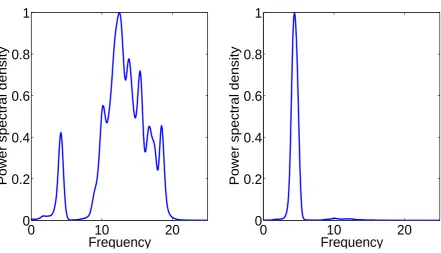
The method that is used in order to calculate the power spectral densities (PSDs) which follow is the Welch method based on time averaging over short, modified periodograms which could decolour the effect of different random excitation inputs [16]. The signals are split into sections and the periodograms of each section are averaged. Through the Welch method these data sections are overlapped and a window, such as the Hanning window is applied in order to filter each section. The overlapping of the signal sections is usually either 50% (as in this paper) or 75%.

Fig.2 shows the results of PSDs for the simulated physical variables. Both modes are present in the PSDs for the transformed coordinates which shows that the system is clearly not uncoupled. For all the graphs the vertical axe is thePSD of displacementand thefrequency is in Hz.

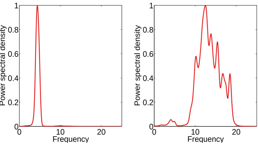
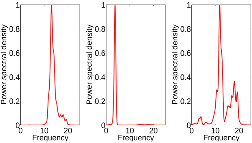
As can be seen in Fig.3, PCA fails in decoupling the nonlinear system (standard linear modal analysis) but kernel ICA, as seen in Fig.4, is successfully decoupling the nonlinear system into two SDOF systems due to the removal of the higher order statistical dependence. Standard linear modal analysis is equivalent to PCA in this case as the mass matrix is diagonal.

0

10

20

0

0.2

0.4

0.6

0.8

1

Power spectral density

Frequency

0

10

20

0

0.2

0.4

0.6

0.8

1

Power spectral density

Frequency

Figure 2: PSDs for physical variables.

0

10

20

0

0.2

0.4

0.6

0.8

1

Power spectral density

Frequency

0

10

20

0

0.2

0.4

0.6

0.8

1

Power spectral density

Frequency

0

10

20

0

0.2

0.4

0.6

0.8

1

Power spectral density

Frequency

0

10

20

0

0.2

0.4

0.6

0.8

1

Power spectral density

Frequency

Figure 4: PSDs for transformed variables: Kernel ICA.

5

A three-degree-of-freedom system

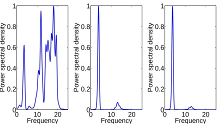
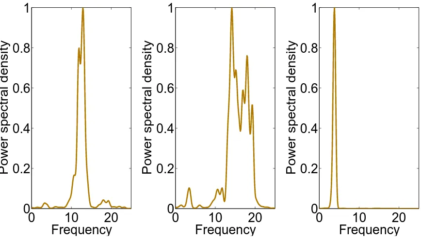
In order to validate the results further, a more complicated system in terms of degrees of freedom and increased cubic nonlinearity is discussed (see Fig.5). As can be seen in Figs.6-8, both PCA and kernel ICA lack in efficiency and performance in decoupling the nonlinear modes of the system. This is the reason that a novel approach to structural dynamics is introduced next in the form of the local linear embedding method. The system of interest will be a nonlinear three-DOF lumped parameter system. Data were simulated using a fixed-step4th_{-order Runge-Kutta algorithm and the excitation was chosen to be a Gaussian white noise}

sequence with zero mean and unit variance. The model parameters adopted were: m = 0.1, c1 = 0.01,

c2 = 0.02,c3 = 0.03,k1 = 50,k2 = 150,k3 = 300,knl= 105. The nonlinearity that is assumed is cubic.

Figure 5: Nonlinear three-DOF lumped parameter system.

5.1 Nonlinear manifold learning via locally linear embedding

0

10

20

0

0.2

0.4

0.6

0.8

1

Power spectral density

Frequency

0

10

20

0

0.2

0.4

0.6

0.8

1

Power spectral density

Frequency

0

10

20

0

0.2

0.4

0.6

0.8

1

Power spectral density

Frequency

Figure 6: PSDs for physical variables.

0

10

20

0

0.2

0.4

0.6

0.8

1

Power spectral density

Frequency

0

10

20

0

0.2

0.4

0.6

0.8

1

Power spectral density

Frequency

0

10

20

0

0.2

0.4

0.6

0.8

1

Power spectral density

Frequency

0

10

20

0

0.2

0.4

0.6

0.8

1

Power spectral density

Frequency

0

10

20

0

0.2

0.4

0.6

0.8

1

Power spectral density

Frequency

0

10

20

0

0.2

0.4

0.6

0.8

1

Power spectral density

Frequency

Figure 8: PSDs for transformed variables: Kernel ICA.

Other very strong methods can be applied in such complex nonlinear manifolds such as nonlinear principal component analysis via the usage of auto-associative neural networks [11, 19, 20]. The usage of such methods is SHM can be seen in [21]. For the current study LLE is used as it is a novel introduction into nonlinear modal analysis and a much simpler tool.

An extensive overview of the algorithm can be found in [17, 18]. Briefly and for the purposes of this paper a short description is discussed.

The LLE method is based on simple geometric intuition. If the observations consist ofN real-valued vectors

{xi}with dimensionsDand they are sampled from a smooth underlying nonlinear manifold, then each data

point and its neighbours is expected to lie on or close to a locally formed patch of the manifold. This local geometries can be characterised by finding linear coefficients that can reconstruct each data point with respect to each set of neighbours.

If one establishesK nearest neighbours per data point then the reconstruction error is given by the cost function:

error(W) =X

i

{xi} −

X

j

[Wij]{xj}

2 (11)

where[Wij]is the weight contribution of thejthdata point to theithreconstruction. In order to compute

these weights the cost function has to be minimised under the following constraints. The reconstruction errors that are subject to the constrained weights should be invariant to rotations and rescaling. In turn, in order that the LLE algorithm preserve this invariant manifold idea as a final step of the method, each measurement{xi}

should be mapped to lower dimensional vector{Yi}that minimises the cost function:

error(Y) =X

i

{Yi} −

X

j

[Wij]{Yj}

are optimised.

In Fig.9 the LLE method is shown to the successfully decoupling the modes as it was able to unfold and learn the underlying nonlinear manifold.

0

10

20

0

0.2

0.4

0.6

0.8

1

Power spectral density

Frequency

0

10

20

0

0.2

0.4

0.6

0.8

1

Power spectral density

Frequency

0

10

20

0

0.2

0.4

0.6

0.8

1

Power spectral density

Frequency

Figure 9: PSDs for transformed variables: Local linear embedding.

6

Conclusion

The purpose of this paper is to highlight the key utility of some machine learning methods, not only for dynamic analysis of structure but as well as a method of reduction for nonlinear mechanical systems. The main benefit of the approach taken here is that complicated algebraic analysis is not necessary. Furthermore, the physical equations of the system are not needed.

The biggest advantage of these methods is that one can built for several datasets the nonlinear subspace manifold only once and it then can be used for future testing datasets. As a result, this machine learning approach is suited to experimental investigation of nonlinear systems using only the measured output responses. A further work in the form of a journal article is under preparation where other multi-degree of freedom systems are investigated as well as experimental validation of the methods.

Acknowledgments

References

[1] G. Kerschen, J.-c. Golinval, A. F. Vakakis, L. A. Bergman,The method of proper orthogonal decomposi-tion for dynamical characterizadecomposi-tion and order reducdecomposi-tion of mechanical systems: an overview, Nonlinear dynamics 41 (1-3) (2005) 147–169.

[2] A. Vakakis,Non-linear normal modes (NNMs) and their applications in vibration theory: an overview, Mechanical systems and signal processing 11 (1) (1997) 3–22.

[3] K. Worden, G. R. Tomlinson,Nonlinearity in structural dynamics: detection, identification and mod-elling, CRC Press, 2000.

[4] K. Worden, G. Tomlinson,Nonlinearity in experimental modal analysis, Philosophical Transactions of the Royal Society of London. Series A: Mathematical, Physical and Engineering Sciences 359 (1778) (2001) 113–130.

[5] K. Worden, P. Green,A Machine Learning Approach to Nonlinear Modal Analysis, in: Dynamics of Civil Structures, Volume 4, Springer, 2014, pp. 521–528.

[6] R. M. Rosenberg, The normal modes of nonlinear n-degree-of-freedom systems, Journal of applied Mechanics 29 (1) (1962) 7–14.

[7] S. W. Shaw, C. Pierre,Normal modes for non-linear vibratory systems, Journal of sound and vibration 164 (1) (1993) 85–124.

[8] S. A. Neild, D. J. Wagg, Applying the method of normal forms to second-order nonlinear vibration problems, Proceedings of the Royal Society A: Mathematical, Physical and Engineering Science 467 (2128) (2011) 1141–1163.

[9] F. Poncelet, G. Kerschen, J.-C. Golinval, D. Verhelst,Output-only modal analysis using blind source separation techniques, Mechanical Systems and Signal Processing 21 (6) (2007) 2335–2358.

[10] C. M. Bishop, et al.,Pattern recognition and machine learning, Vol. 4, springer New York, 2006.

[11] C. M. Bishop, et al.,Neural networks for pattern recognition, Clarendon press Oxford, 1995.

[12] I. T. Nabney,NETLAB: algorithms for pattern recognition, Springer, 2004.

[13] A. Hyv¨arinen, E. Oja,A fast fixed-point algorithm for independent component analysis, Neural computa-tion 9 (7) (1997) 1483–1492.

[14] H. G¨avert, J. Hurri, J. S¨arel¨a, A. Hyv¨arinen,The FastICA package for MATLAB, Lab. of Computer and Information Science, Helsinki University of Technology.

[15] F. R. Bach, M. I. Jordan,Kernel independent component analysis, The Journal of Machine Learning Research 3 (2003) 1–48.

[16] P. Welch,The use of fast Fourier transform for the estimation of power spectra: a method based on time averaging over short, modified periodograms, Audio and Electroacoustics, IEEE Transactions on 15 (2) (1967) 70–73.

[17] L. K. Saul, S. T. Roweis, An introduction to locally linear embedding, unpublished. Available at: http://www. cs. toronto. edu/˜ roweis/lle/publications. html.

[18] S. T. Roweis, L. K. Saul,Nonlinear dimensionality reduction by locally linear embedding, Science 290 (5500) (2000) 2323–2326.

pp. 439–444.