Stationary relativistic jets

R E S E A R C H

Open Access

Stationary relativistic jets

Serguei S Komissarov

_{, Oliver Porth}

_{and Maxim Lyutikov}

Abstract

In this paper we describe a simple numerical approach which allows to study the structure of steady-state axisymmetric relativistic jets using one-dimensional time-dependent simulations. It is based on the fact that for narrow jets withvz≈cthe steady-state equations of relativistic magnetohydrodynamics can be accurately approximated by the one-dimensional time-dependent equations after the substitutionz=ct. Since only the time-dependent codes are now publicly available this is a valuable and efficient alternative to the development of a high-specialised code for the time-independent equations. The approach is also much cheaper and more robust compared to the relaxation method. We tested this technique against numerical and analytical solutions found in literature as well as solutions we obtained using the relaxation method and found it sufficiently accurate. In the process, we discovered the reason for the failure of the self-similar analytical model of the jet reconfinement in relatively flat atmospheres and elucidated the nature of radial oscillations of steady-state jets.

Keywords: jets; relativity; magnetic fields; hydrodynamics; numerical methods

1 Introduction

Highly collimated flows of plasma from compact ob-jects of stellar mass, like young stars, neutron stars and black holes, as well as supermassive black holes resid-ing in the centers of active galaxies is a wide-spread phe-nomenon which has been and will remain the focal point of many research programs, both observational and the-oretical. Some features of these cosmic jets, like moving knots, are best described using time-dependent fluid mod-els. However, most of these jets have sufficiently regular global structure, which is indicative of steady production and propagation and promotes development of stationary models. Such models are also easier to analyze, and they are very helpful in our attempts to figure out the key fac-tors of the jet physics.

The simplest approach to steady-state flows is to com-pletely ignore the variation of flow parameters across the jet. This allows to reduce the complicated system of non-linear partial differential equations (PDEs) describing the jet dynamics to a set of ordinary differential equations

*_{Correspondence: [email protected]}

1_{School of Mathematics, University of Leeds, Leeds, LS29JT, UK}

2_{Department of Physics and Astronomy, Purdue University, West Lafayette,} 47907-2036, USA

Full list of author information is available at the end of the article

(ODEs) which can be integrated more easily (e.g. Bland-ford and Rees ; Komissarov ). A similar reduc-tion in the dimensionality is achieved in self-similar mod-els, where unknown functions depend only on a combi-nation of independent variables known as a self-similar variable. This also allows to reduce the original PDEs to a set of ODEs (e.g. Blandford and Payne ; Vlahakis and Tsinganos ). While providing important test cases and useful insights, this approach is not sufficiently robust - boundary and other conditions that select such excep-tional solutions are not always present in nature.

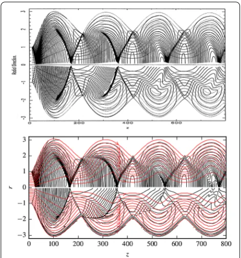
As it is well known to engineers working on aircraft jet engines, supersonic jets naturally develop quasi-periodic stationary chains of internal shocks, similar to what is shown in Figure . These shocks emerge as a part of the adjustment of the jet pressure to that of the surround-ing air. Interestsurround-ingly, bright knots are often seen in cos-mic jets and they are often interpreted as shocks (e.g.Falle and Wilson ; Daly and Marscher ; Gómez and Marscher ; Arshakian et al. ; Walker ). Some of these knots are known to be traveling and they must be part of the jet’s non-stationary dynamics. Others ap-pear to be static and hence connected to the underlying quasi-steady-state structure of these cosmic jets. Quite of-ten, the knots form quasi-periodic chains, reminiscent of those seen in aerodynamic jets. If the similarity is not

Figure 1 Reconfinement of theMj= 15,Tj=√10×1013_Kjet.

The top panel is a reproduction of Figure 3 from B94. The bottom panel shows the solution obtained with our method. In each panel, the top halves show 50 pressure contours (spaced by the factor of 1.18) and the bottom halves show the temperature parameter

τ≡ρh/(ρh–p) in 50 contours (spaced by the factor of 1.003). The light gray lines are streamlines.

cidental, then these knots are also related to the process of pressure adjustment. In particular, we expect the powerful cosmic jets to be expanding freely soon after leaving their central engines and to become confined by external pres-sure again only much later (e.g.Daly and Marscher ; Komissarov and Falle ). The first shock driven into the jet by the external pressure is called the reconfinement shock. Given the growing observational evidence of sta-tionary knots in cosmic jets, there has been a increase of interest to the reconfinement process among theorists in recent years (e.g.Nalewajko and Sikora ; Nalewajko ; Bromberg and Levinson ; Bromberg and Levin-son ; Kohler et al. ; Kohler and Begelman ; Kohler and Begelman ). One of the key aims of these studies was to come up with approximate analytical or semi-analytical solutions for the structure of steady-state jets.

Obviously, such shocked flows cannot be described by one-dimensional (D) and self-similar models, which we mentioned earlier, and more complex, at least two-dimensional (D), models have to be applied instead. The system of steastate equations of compressible fluid dy-namics, not to mention magnetohydrodydy-namics, is already very complicated and generally requires numerical treat-ment. One of the ways of finding its solutions involves

integration of the original time-dependent equations in anticipation that if the boundary conditions are time-independent then the time-dependent numerical solution will naturally evolve towards a steady-state (e.g. Ustyu-gova et al. ; Komissarov et al. ; Tchekhovskoy et al. ). One clear advantage of this approach is that it allows to use standard codes for time-dependent fluid dynamics. Such codes are now well advanced and widely available. However, this type of the relaxation approach is characterized by slow convergence and hence rather ex-pensive.

In order to speed up the convergence, one can use other relaxation methods, which are developed specifically for integrating steady-state equations (e.g.May and Jameson ). They often involve a relaxation variable which is called ‘pseudo time’. However, this time evolution is not realistic but designed to drive solutions towards a steady-state in the fastest way possible. The only disadvantage of this approach is that it involves development of a spe-cialised computer code dedicated to solving only steady-state problems. The authors are not aware of such codes for relativistic hydro- and magnetohydrodynamics.

For supersonic flows, the system of steady-state equa-tions turns out to be hyperbolic, with one of spatial coor-dinates playing the role of time (Glaz and Wardlaw ). (In the case of magnetic jets, the speed of sound is re-placed with the fast magneto-sonic speed and we classify flows as sub-, tran-, or super-sonic based on its value com-pared to the flow speed.) In this case, one can find steady-state solutions utilising numerical methods which were de-signed specifically for hyperbolic systems, like the method of characteristics or ‘marching’ schemes. These methods have been used in the past in applications to relativistic jets (e.g.Daly and Marscher ; Wilson and Falle ; Wilson ; Bowman ; Bowman et al. ) but pub-licly available codes do not exist yet. Their development is as time-consuming as that of time-dependent codes whereas the range of applications is much more limited. This explains their current unavailability. Moreover, when flow becomes subsonic, even very locally, this approach fails.

simulations, no special effort is needed to preserve the magnetic field divergence-free and the computational er-rors associated with multi-dimensionality are eliminated. As the result, more extreme conditions can be tackled. Here we focus only on relativistic jets, because of our in-terest to AGN and GRB jets, but we see no reason why this approach cannot be applied to non-relativistic hyper-sonic jets as well. Our approach is closely related to the so-called ‘frozen pulse’ approximation, which also utilizes the similarity between the steady-state and time-dependent equations describing ultra-relativistic flows (Piran et al. ; Vlahakis and Königl ; Sapountzis and Vlahakis ). In this approximation, the steady-state equations are used to analyze the dynamics of time-dependent flows. The similarity between D time-dependent models and D steady-state jet solutions has been noted before, in partic-ular in Matsumoto et al. ().

In order to study the potential of this new approach we have carried out a number of test simulations and com-pared the results obtained in this way with both analytical models and numerical solutions obtained with more tradi-tional methods. The results are very encouraging and allow us to conclude that this method is viable and can be used in a wide range of astrophysical applications.

2 Approximation

We start by writing down the time-dependent equations of Special Relativistic Magnetohydrodynamics (SRMHD). In this section we use units where the speed of lightc=  and the factor /πdoes not appear in the expression for the electromagnetic energy density. The components of vec-tors and tensors are given in normalized bases. The evolu-tion equaevolu-tions of SRMHD include the continuity equaevolu-tion

∂tρ+∇ ·(ρv) = , ()

the Faraday equation

∂tB+∇ ×E=  ()

and the energy-momentum equation

∂tTtμ+∇jTjμ= , ()

where

Tνμ=T_hdνμ+T_emνμ ()

is the total stress-energy-momentum tensor,

T_hdνμ=wuνuμ+pgνμ ()

is stress-energy-momentum tensor of matter and the com-ponents of the electromagnetic stress-energy-momentum

tensor are

Ttt em=

E_+B_{/, ()}

T_emti = (E×B)i, ()

T_emij = –EiEj+BiBj+ 

E+Bgij. ()

In these equations, B and E are the vectors of magnetic and electric fields respectively,p,ρ andware the thermody-namic pressure, rest-mass density of matter and relativis-tic enthalpy of matter respectively, v is the velocity vector,

is the Lorentz factor and g is the metric tensor of space. These equations are to be supplemented with Equation of Statew=w(ρ,p) and the Ohm’s law of ideal MHD

E= –v×B. ()

Finally, the magnetic field is divergence-free

∇ ·B= . ()

In this analysis, we focus on axisymmetric jets and adopt a cylindrical coordinate system with thezaxis coincident with the jet symmetry axis. We consider only narrow jets, so that

r

z. ()

We also constrain ourselves with a relatively simple mag-netic configurations where the divergence-free condition leads to

Br Bz

r

z. ()

In axisymmetry, the steady-state Faraday equation implies

Eφ_{= . When combined with Eq. (), this result yields}

vr vz =

Br

Bz . ()

Thus, the radial components of both the magnetic field and the velocity vectors are small compared to their axial com-ponents.

We also assume thatvφ_{. In fact, in the case of} mag-netically accelerated jets,

vφ_(r lc/r)

whenrrlc, the radius of light cylinder (see Eq. () in Komissarov et al. ()). Thus, this is a good approxima-tion for astrophysical jets. For a highly relativistic flow, the conditionvz_vr_,vφ_means

Following the standard flux freezing argument, along the jet Bφ_/Bz_(r

j/rlc)–, where andrjis the jet radius (This argument does not apply to turbulent jets, which are non-axisymmetric and allow non-trivial conversion of compo-nents.). Hence one may argue that far away from the cen-tral engine

BφBz. ()

In order to introduce the key idea of our approach we consider first the steady-state continuity equation:

∂z

ρvz+∇rρvr= . ()

Using the condition () we may replacevz_{with unity. This}

makes Eq. () identical to the D time-dependent version of the continuity equation. In order to stress this point we replacezwithtand write:

∂t(ρ) +∇r

ρvr= . ()

Similarly, all D steady-state equations can be approx-imated by the corresponding D time-dependent equa-tions.

Let us show this for the equations of magnetic field. The D version of the divergence free condition reads

∂r

rBr=  or rBr= const.

Thus if Br vanishes outside of the jet, which is expected when it is in direct contact with ISM, then one has to put

Br_{=  everywhere in the D model. As we shell see, the}

terms involvingBr_{are sub-dominant in all other equations}

and hence this is a reasonable simplification. Moreover, once the D solution is found, one can substitute the deter-minedBz_{(r,z) into the D divergence free condition and}

solve it forBr_{(r,z). The result can then be used to verify}

thatBr_(r,z)Bz_(r,z).

Theφcomponent of the Faraday equation can be written as

∂tBφ–rBi∂i

vφ

r

+∂i

viBφ= , ()

wherei=r,z. In steady-state, the first term vanishes, the next two terms are of the order Bz_vφ_{/z and small} com-pared to the last two terms, which are of the orderBφ_vz_/z.

Removing these small terms we obtain the approximate steady-state equation

∂z

vzBφ+∂r

vrBφ= . ()

Finally, we replacevzwith unity,zwitht, and obtain

∂tBφ+∂r

vrBφ= . ()

This is indeed the D version of theφ component of Eq. (). Now consider thezcomponent of the Faraday equa-tion,

∂tBz–Bi∂ivz+



r∂i

rviBz= . ()

The last two terms of this equation are of the order

vz_Bz_{/z B}z_{/z. On the other hand, the second and the}

third terms are much smaller because of the special sta-tus of vz_{, which is approximately constant, and hence} Bz_∂

zvzBz(vz/z). Removing these small terms, we obtain

the approximate steady-state equation

∂z

vzBz+

r∂r

rvrBz= . ()

Now once again we replacevz with unity andzwithtto obtain

∂tBz+



r∂r

rvrBz= , ()

which is the D version of thezcomponent of Eq. (). Finally, we analyze the energy-momentum equations. These can be written as

∂tTtμ+∂zTzμ+∇rTrμ= , ()

so the steady-state versions are

∂zTzμ+∇rTrμ= . ()

These already have the same form as the D time-depen-dent equations, so we only need to show that

TzμTtμ. ()

Let us start with the hydrodynamic contribution. First, we notice that

T_hdtt =w–pw as;

Ttz hd=w

_vz_w _asvz_.

Thus,T_hdztTtt

hd. Then we notice that

T_hdti =wvi;

T_hdzr =wvzvrwvr;

T_hdzz=wvzvzwvz;

Thus,Tzi hdThdti.

Now we inspect the electromagnetic contributions. First, we find good estimates for the components of electric field. From Eq. () it follows that

and

Ez_=Br_vφ_–Bφ_vr_Er_.

In fact, it is easy to show that

Ez–Bφvr. ()

Indeed, for magnetically accelerated jets Bφ _rBz _(e.g.

Komissarov et al. ) forrrlc. Hence

vrBφvr rBz(r/rlc)BrBrBrvφ.

Using these estimates we find that

T_emtt = 

E+BBφ;

T_emtz = (E×B)zErBφBφ,

and henceTzt

emTemtt. Moreover,

T_emzz = –E_z+B_z+E _+B

 B

 φ,

and henceTzz

emTemtz as well. Next we show that T zφ em

Temtφ. Indeed,

T_emtφ =EzBr–ErBz–ErBz,

and

T_emzφ= –EzEφ+BzBφ–BzEr.

Finally, we show that T_emzr T_emtr . First, we find straight away that

T_emtr = –EzBφ and T_emzr = –EzEr+BzBr.

SinceEzErEzBφ_{, we only need to show thatB}z_Br_is

sig-nificantly smaller compared to these terms. This is indeed the case asBzBrvrB_z whereas using Eqs. () and () we obtainEz_Er_v

rBφvrBz.

Thus, within our approximation the steady-state D equation of energy-momentum reduces to

∂tTtμ+∇rTrμ= , ()

which is the D time-dependent energy-momentum equa-tion.

Given that in relativistic fluid dynamics small differences between the magnitudes of energy and momentum may result in huge variations of Lorentz factor and even lead to inconsistency, one could feel uneasy about the approx-imations we make. However, the final result isexactlythe

system of D time-dependent SRMHD and this means that self-consistency is not compromised. For example, the flow speed will not exceed the speed of light because of the errors of our approximation.

Our approach is similar to ‘marching’ - we compute so-lution for a downstream jet cross-section using only the previously found solutions for upstream cross-sections. Strictly speaking, this requires the flow to be super-sonic for unmagnetized jets and super-fast-magnetosonic for magnetized ones (Wilson and Falle ; Dubal and Pan-tano ). However, in our derivations we never had to utilize this condition. This suggests that it is not required when we wish to find only approximate solutions. For ex-ample, one may argue that the fact that information can propagate upstream does not necessarily imply that this always has a strong effect on the flow - the upstream-propagating waves could be rather weak. If so, we may still apply our method to jets where the supersonic con-dition is not fully satisfied, but we always need to check that the conditions ()-() of our approximation hold for obtained solutions.

3 Numerical implementation

The analysis of Section  shows that as long as they are ap-plied to narrow jets with high Lorentz factor, the axisym-metric steady-state equations of SRMHD are very close to D time-dependent equations of SRMHD in cylindrical ge-ometry. This suggests that it may be possible to use time-dependent simulations with D SRMHD codes to study the D structure of steady-state jet solutions. However in or-der to be able to do this, we also need to find a way of ac-commodating the D boundary conditions of steady-state problems in such simulations.

For D supersonic flows we need to fix all flow param-eters at the jet inlet and impose some conditions at the jet boundary, consistent with it being a stationary contact wave. No boundary conditions are needed for the outlet boundary - its flow parameters are part of the solution. In the corresponding D problem, the D boundary tions at the inlet boundary simply become the initial condi-tions of the D Cauchy problem. The final D solution cor-responds to the slice of the D solution at the outlet bound-ary. As to the contact discontinuity at the D jet boundary, the situation is not that trivial.

Suppose that the total pressure at this boundary is a function ofz,p=pb(z). When we replacezwithtthis be-comesp=pb(t). Thus we need somehow to impose

In order to locate the boundary separating the jet from the external gas, we employ a simplified version of the level-set method (Osher and Sethian ; Sethian and Smereka ). Namely, we introduce the passive scalarτ, which satisfies the advection equation

∂t(ρτ) +



r∂r

rvrρτ= . ()

The initial solution has a smooth distribution of this scalar

τ=



 –tanhr–rj

, ()

with the valueτ = . corresponding to the jet boundary (In the test simulations, we used = .rj.). During the

simulations, the conditionτ< . was used to identify the external gas.

After the reset, the D jet boundary is no longer a con-tact but a more general discontinuity. In particular, the jet plasma will generally have radial velocity component. If it is positive, but in the external gas it is set to zero, then a shock wave will launched into the jet when this disconti-nuity is resolved. If it is negative, then this will be a rar-efaction wave. On the one hand, this reflects how the in-formation about changing environment is communicated to the interior of a steady-state jet. On the other hand, in D simulations the strength of the emitted wave depends on the external density - higher density, and hence lower temperature, will result in stronger waves moving into the jet. This is obviously not so for D steady-state jets, which react only to the external pressure. Thus additional mea-sures need to be undertaken. First, in order to negate the effect of the radial velocity jump at the jet boundary, the radial velocity of the external gas is reset not to zero but to its value at the last jet cell. Second, in order reduce the role of the external gas inertia, it helps to set its density to a low value, so that its sound speed becomes relativistic. Although we have not tried this, one could set the poly-tropic index of the external gas to= , which would make the sound speed of ultra-relativistically hot gas equal to the speed of light.

4 Examples

4.1 Bowman’s jet

To test the validity of our approach, we first use our method to reproduce the numerical steady-state solutions for supersonic unmagnetized jets obtained by Bowman (), B, using the marching scheme described in Wil-son (). In this study pressure-matched uniform jets with zero opening angle are injected into an atmosphere with the pressure distribution

p(z) =p

z zs – +  –zs

z zs zc  ()

withzs= ,zc= . According to this equation, the ex-ternal pressure initially decreases almost as fast as∝z–

but atz>zcbecomes uniform. The initial jet radiusr=  and the injection nozzle is located atz=zs. The equation of state is that of Synge () for an electron-proton plasma. The initial jet pressurepj=p. For the comparison we se-lected the model with the Mach numberMj=  and the initial temperatureTj=

√

×_{K. At such a high} tem-perature the EOS of electro-proton plasma is almost the same as that of the pure proton gas. The latter was used in our simulations.

Bowman’s solution is shown in the top part of Figure . As the external pressure decreases rapidly, the jet quickly becomes under-expanded and enters the phase of almost free expansion. When it enters the outer region of con-stant pressure it becomes over-expanded and a reconfine-ment shock is pushed towards its axis, where it gets re-flected. Gas passed though these two shocks becomes hot and its pressure rises. As a result, the jet becomes some-what under-expanded again and begins to expand for the second time. Then it becomes over-expanded again and another shock is pushed into the jet and so on.

In the bottom part of this figure, we show the results of our D simulations for this jet using exactly the same visu-alization technique as in the original paper. The agreement between the two solutions is quite remarkable. A very good match for the maximal radial extension and the oscillation-length of the jet is obtained. The successive reconfinement shocks are somewhat sharper than in B, most likely due to the application of a shock-capturing scheme. We checked our approach against other numerical models of B as well. In all models, the results for profile of jet ra-dius and Mach number are in good agreement. Noticeable but still minor differences arise only for the colder models, most likely due to the different equation of state used in our simulations.

4.2 Self-similar models of jet reconfinement

The problem of reconfinement of initially free-expanding steady-state jets is quite important and a number of au-thors have tried to find simple analytic of semi-analytic so-lutions. Falle () and Komissarov and Falle () used the Kompaneets approximation, which assumes that the gas pressure immediately downstream of the reconfine-ment shock is equal to the external pressure at the same distance, to derive a simple ODE for the shock radius. As-suming particular flow profiles in the shocked layer, one can also determine the location of the jet boundary (e.g.

Figure 2 Ultra-relativistically hot jets (Kohler et al. 2012; Kohler and Begelman 2015) in power-law atmospheres withκ= 8/3, 7/3 and 2 (from left to right).The color-coded images show the distribution of the Lorentz factor. The initial Lorentz factor is0= 50 and opening angle θ0= 1/0.

layer. This assumption is more suitable for the case where the reconfinement shock never reaches the jet axis, be-cause otherwise the distance where this occurs sets a char-acteristic length scale.

KBB studied jets with ultra-relativistic equation of state (w= p,γ = /), propagating in a power-law atmo-sphere,

p=p

z z

–κ

. ()

These jets emerge from a nozzle atz=zwith the Lorentz factor, opening angle θ= / and pressurep. The initial velocity distribution correspond to a conical flow originating fromz=  and hence the initial jet radiusr=

ztan(θ). They could only find self-consistent solutions for /≤κ<  and later argued that forκ< / the entropy of the shocked layer must increase with the distance along the jet in order for the solution to be consistent with the energy conservation (Kohler and Begelman ). They proposed that this additional heating is caused by multi-ple shocks driven into the flow as it gradually collimates.

We selected the KBB model withκ= / and=  and made simulations on a uniform grid with only  cells (each run took only several CPU minutes on a laptop using only one core of its processor). Our results are shown in the first panel of Figure , which should be compared with

Figure  in KBB. Again we find a very good agreement between the models - atz=  we have got the jet radiusrj≈ . and the shock radiusrs≈., whereas in KBB

rj= . andrs= ..

In order to understand the difference between the cases withκ> / andκ< /, we also computed models with

Figure 3 Ultra-relativistically hot jets (Kohler et al. 2012; Kohler and Begelman 2015) in power-law atmospheres withκ= 8/3, 7/3, and 2 (from left to right).The color-coded images show log10(pρ–γ). The dark blue region along the jet boundary is obviously a numerical artifact as its

entropy is lower than that of the initial solution anywhere on the grid.

The plots in Figure  also reveal a thin layer of decreased entropy stretching along the jet boundary. As in this layer the entropy is lower than anywhere in the initial solution, this is definitely a numerical artifact. We have checked that it becomes less pronounced with increased numerical res-olution. Moreover, this layer forms well inside the jet and thus its origin is not related to the resetting procedure but is a property of our time-dependent code.

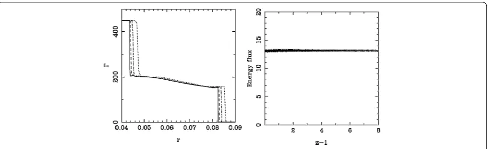
We choose the model withκ= , to illustrate the conver-gence and accuracy of our numerical solutions. The left panel of Figure  shows the Lorentz factor distributions found atz=  for runs with different number of grid cells in the computational domain, increasing from  to , cells. As one can see, the solutions converge as in a first-order accurate scheme. The right panel shows the evolu-tion of the total energy flux along the jet. It remains fairly constant, as expected for a conserved quantity. As the jet boundary jumps from one cell to another, a low level noise is introduced to this integral variable.

4.3 Magnetized jets. 1D versus 2D solutions

The steady-state structure of magnetized jets is more com-plex, mainly due to the non-trivial contribution of the magnetic tension to the force balance. A number of au-thors have tackled this problem analytically using vari-ous approximations (e.g.Zakamska et al. ; Lyubarsky

; Lyubarsky ; Kohler and Begelman ). How-ever, none of these studies deliver a model suitable for de-tailed testing of our numerical approach. Dubal and Pan-tano () studied the steady-state structure of relativis-tic jets with azimuthal magnerelativis-tic field using the method of characteristics. This would be a good test case but the setup of their simulations is ambiguous. We have tried sev-eral variants of the setup but each time failed to repro-duce the results. The mechanisms of magnetic collimation and acceleration of relativistic jets were studied numeri-cally by Komissarov et al. (), Komissarov et al. () and Tchekhovskoy et al. () using a ‘rigid wall’ outer boundary. While this allows for a well-controlled experi-ment, Komissarovet al.() have shown that the con-nection between the shape of the boundary and the ex-ternal pressure gradient is not straightforward, with sig-nificant degeneracy. For this reason, we concluded that in the magnetic case the best way of testing the performance of our D approach would be via new D axisymmetric time-dependent simulations using the relativistic AMR-VAC code (Keppens et al. ; Porth et al. ).

Figure 4 Accuracy of the ultra-relativistic hot jets solution for the model with atmospheres withκ= 2.The left panel shows the Lorentz factor atz= 9 for models with 150 (dotted), 300 (dot-dashed), 600 (dashed line) and 1,200 (solid line) grid points. The right panel show the total energy flux as a function of the distance from the nozzle for the model with 300 grid points.

rest mass density of its particles is not negligibly small. The jet structure at the inlet is that of a cylindrical jet in mag-netostatic equilibrium, which satisfies the following force balance equation

dpt dr +

bφ

r drbφ

dr = , ()

wherebφ_=Bφ_{/is the azimuthal component of the} mag-netic field as measured in the fluid frame using normalized basis andptis the sum of the gas pressure and the magnetic

pressure due to the axial magnetic fieldBz (Komissarov

). Equation () has infinitely many solutions - given a particular distribution forbφ_{(r) one can solve this equation} for the corresponding distribution of the pressure pt(r).

We adopted the ‘core-envelope’ solution of Komissarov ():

bφ(r) = ⎧ ⎨ ⎩

bm(r/rm); r<rm, bm(rm/r); rm<r<rj,

; r>rj,

()

pt(r) =

⎧ ⎨ ⎩

p[α+βm ( – (r/rm)

_{)]; r<r} m,

αp; rm<r<rj,

p; r>rj,

()

where

βm=

p

b m

, α=  – (/βm)(rm/rj), ()

rj is the jet radius andrm is the radius of its core (Note

a typo in the expression forα in Komissarov ().). As one can see, the core is pinched and in the envelope the magnetic field is force-free. This may be combined with any distribution of density and axial velocity. We imposed

ρ=ρand

(r) =

 – (r/rj)ν

+ (r/rj)ν, ()

with ν= ; this gives an almost ‘top-hat’ velocity profile. The velocity vector is set to be aligned with the jet axis, so

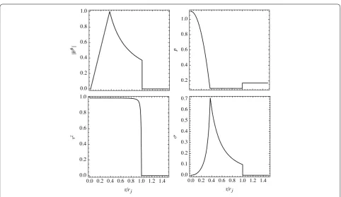
vr=vφ= . This solution is illustrated in Figure .

We considered two models, A and B. In the models A, the magnetic field is purely azimuthal and the other parame-ters arerj= ,rm= .,bm= ,ρ= ,z= ,βm= .,

= . The local magnetization parameterσ=b/wdoes not exceedσmax= . in this model and thus the jet is only moderately magnetized. The jet core is relativistically hot, with the gas pressure reachingpmax=ρat the axis, which opens the possibility of efficient hydrodynamic accelera-tion once the jet is allowed to expand. In the simulaaccelera-tions we used the adiabatic equation of statew=ρ+ (γ/γ – )p

withγ = /.

In model B, this configuration is modified to include nonvanishing longitudinal magnetic fieldBz. In particular,

we considered the case where the gas pressurep=αp ev-erywhere within the jet and

Bz=

p[βm( – (r/rm)

_{)]; r<r} m,

; r>rm,

()

which keeps pt unchanged. In this model, the magnetic

field is force-free not only in the envelope but also in the core. The other parameters of this model that differ from those of model A areρ= . andβm= .. The

corre-sponding magnetization is much higher, withσmax= . Model B turned out too stiff for our D code, but pre-sented no problems in D simulations. For this reason we compare here the D and D results for model A only. In these simulations we used the atmosphere withκ= . The computational domain is rjin the radial direction and

Figure 5 Initial radial structure of the magnetized jets in the test simulations described in Section 4.3.

First, let us describe the overall jet structure found in these simulations. Initially, as the jet enters the region of rapidly declining external pressure, it expands rapidly and a rarefaction wave moves towards its axis. Eventually, the jet becomes over-expanded, its expansion slows down, and a reconfinement shock sets in. It reaches the axis atz≈

, gets reflected and then returns to the jet boundary at

z≈ (see Figure ).

To quantify the convergence of the D simulations we carried out simulations with three different resolution and used this data to determine the grid-convergence index

η≡–ln _|

f–f| |f–f|

/ln, ()

wheref,fare solutions with doubled and quadrupled res-olution compared tofand|fa–fb|is the difference be-tween two solutions in theLnorm. We found thatη≈, as this is expected for a TVD scheme in the presence of dis-continuities. At , grid cells in the radial direction, the density contours become visually unchanged on the scale of Figure . The D solution with this resolution was used for comparison with the results of our D simulations. In what follows we refer to it as the ‘converged’ D solution.

The initial solution in our D simulations was con-structed via interpolation of the converged D solution onto the D cylindrical grid. Since we did not include

gravity to balance the pressure gradient in the external at-mosphere, in order to preserve the atmosphere in its ini-tial state the atmospheric parameters were reset to their initial values every time step, just like this was done in the D case. In order to test the convergence of D so-lutions, we made three runs with doubled resolution,Nr=

, , and , cells in the radial direction. The ber of cell in the axial direction was always twice the num-ber of cells in the radial one.

Typically, the D solutions exhibited some evolution at first but then quickly settled into a stationary state. For ex-ample in the case ofNr= , the timestep-to-timestep

relative variation of the conserved flow variables dropped below ×–_{att= , and remained approximately} constant thereafter. Furthermore, the relativeL error of density between timest= , andt= , was .× –, indicating that a stationary state had been reached. The D solutions converge with the grid-convergence in-dexη> . over the entire simulated time.

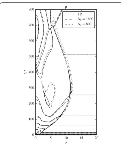
The difference between the converged D solution and the relaxed D solutions withNr=  (dotted lines) and Nr= , (dashed lines) is illustrated in Figure  which

Figure 6 Converged 1D solution for a stationary magnetized jet (solid lines) and two corresponding 2D solutions found via the relaxation method, one with the 1,600_×3,200-resolution (dashed lines) and one with the 800×1,600-resolution (dotted lines).The lines are 10 rest-frame density contours consecutively spaced by the factor of one half from the starting value ofρmax= 1.

The solution involves a reconfinement shock which reaches the jet axis atz≈400.

the parameter

δρ=|ρD–ρD|/ρD. ()

For the D solution withNr=  cells in the radial

direc-tion we obtainδρ%, forNr= ,δρ.%and for Nr= , the relative error decreased toδρ.%. This

shows that the approximation error of our D approach is at the level of no more than %.

4.4 Magnetized jets in power-law atmospheres

Komissarov et al. () derived an approximate equa-tion for the radius of highly magnetized jets, in the limit where it strongly exceeds that of the light cylinder. Using this equation they concluded that in the case of power-law atmosphere with  <κ<  the jet radius increases as

rj∝zκ/. ()

Lyubarsky () developed the theory of Poynting-domi-nated jets further and using more accurate analysis found that the expansion is modulated by oscillations with the

wavelength growing as

λ∝zκ/. ()

These oscillations can be understood as a standing mag-neto-sonic wave bouncing across the jet. Indeed, denote the wave speed as am. Then the jet crossing time isτc= rj/am in the co-moving jet frame andtc=τc in the rest

frame of the atmosphere. As the wave is advected along the jet almost at the speed of light the wavelength of the associated structure is

λ c

am

rj. ()

Since for the jets considered in Komissarov et al. () and Lyubarsky ()amcand∝rj we obtainλ∝ r_j and using Eq. () recover Eq. (). The results (,) are well suited for testing of our approach. To this aim, we carried out additional D simulations with models A and B described in Section ..

Since in model A the jet is not Poynting-dominated, it allows us to explore the regime not covered in Lyubarsky (). To see how sensitive these results may be to the assumptions made in Komissarov et al. () and Lyubarsky () let us consider unmagnetized relativis-tic jets. From the mass conservation law we obtain rj∝

(ρ)–_{. For relativistically cold jets withpρc}_{we have}

const and thus

rj∝zκ/γ, ()

whereas for the hot jets∝rjand thus

rj∝zκ/, ()

where we putγ= /. The last result is the same as for the Poynting-dominated jets. Even for the cold jets the differ-ence is rather minor,e.g.forγ = / the index in Eq. () differs fromκ/ only byκ/ and forγ = / byκ/.

In order findλwe note that for cold jetsa

m∝(p/ρ)∝ z–κ(–/γ)_{and hence Eq. () yields Eq. () independently} of the value ofγ. For hot jets,amconst and Eq. () still

leads to Eq. () if we useγ = /. Thus, the law () for the wavelength of oscillations is very robust.

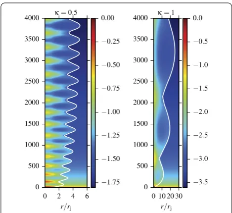
magneto-Figure 7 Structure of steady-state magnetized jets obtained via time-dependent 1D simulations.The plots show the co-moving density distribution for model A withκ= 0.5 andκ= 1. The distance along the vertical axis is defined asz=ct/rj, whererjis the initial jet

radius. The white contour shows the jet boundary, located using the passive scalar.

sonic waves traveling across the jet. In the very beginning, the decrease of external pressure makes the jet under-expanded and a rarefaction wave is launched from the jet boundary towards the jet axis. Behind this wave the radial velocity is positive and the flow expands. The rarefaction reduces the jet pressure and at some point it becomes over-expanded. Now a compression wave is driven inside the jet. Behind this wave the jet expansion slows down and eventu-ally turns into a contraction. The contraction increases the jet pressure and at some point it becomes under-expanded again and then the whole cycle repeats.

The deviation from the force-balance corresponding to the secular jet expansion is due to the finite propagation speed of the waves - as they move across the jet they are also advected downstream by the supersonic flow. As the result, the jet interior reacts to the changes in the external pressure with a delay. It keeps expanding when the internal pressure is already too low and keeps contracting when it is already too high. Asκ increases, the wavelength of the oscillation increases as well. This is expected as the more rapid overall expansion of the jet in an atmosphere with larger κ means that it takes longer for a magneto-sonic wave to traverse the jet, not only as the result of the larger jet radius but also as the result of its higher Mach number (and hence smaller Mach angle).

Overall, this is very similar to the well-known evolution of under-expanded supersonic jets studied in laboratories. Normally, their compressive transverse waves steepen into shocks. In our model A withκ=  we also detect shocks,

but they become progressively weaker, suggesting that they may disappear further out along the jet. Forκ= ., shocks do not form at all. The exact reason for this in not yet clear.

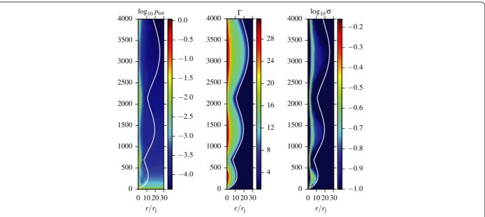
Figure  shows the evolution of other flow parameters in model A withκ = . Both the secular and oscillatory be-havior of the jet radius are mirrored in the variation of the Lorentz factor. The secular expansion leads to secular in-crease of the Lorentz factor as both the thermal and the magnetic energy are converted into the kinetic energy of the flow. The thermal acceleration is most pronounced in the jet core, which is relativistically hot at the inlet. The oscillations of the jet radius lead to additional increase of the Lorentz factor during the expansion phase and its de-crease upon contraction. The left panel of Figure  shows the dynamics of energy fluxes for this jet. These are found via integration over the jet cross-section ofb_vz_–b_bz

for the magnetic energy,ρ_vz _{for the kinetic energy and}

(w–ρ)vz _{for the thermal energy. The results are}

nor-malized to the rest-mass flux, obtained via integration of

ρvz_{. As the result of this normalization, the kinetic}

en-ergy flux has the meaning of mean actual Lorentz factor of the jet, whereas for the thermal energy and magnetic en-ergies these are the gains in the Lorentz factor, which can be achieved upon full conversion of these energies into the kinetic one. The main feature of the plot is a conversion of the thermal energy into the kinetic one (the magnetic en-ergy is highly sub-dominant from the start). This conver-sion is largely completed during the initial phase of mono-tonic expansion, which lasts up toz= . In the second phase, the thermal energy flux is comparable to the mag-netic, and they are being converted to the kinetic energy at more of less the same and rather slow rate. Strong oscilla-tions are superimposed upon this secular evolution, with the kinetic (thermal) energy reaching local maxima (min-ima) at the locations of jet bulging.

Figure  shows the same parameters for the highly mag-netized jet of model B withκ= . In this model, the recon-finement shock is no longer present. This may be related to the fact that in this model the fast magneto-sonic speed is higher and the corresponding jet Mach number is lower, at the inletM compared toM in model A. The lower Mach number is also responsible for the observed lower wavelength of the jet oscillations as it takes less time for the waves to traverse the jet. In this model, the jet is magnetically-dominated and the main feature of its energy balance is a gradual conversion of the magnetic energy into the kinetic one (see the right panel of Figure ).

Figure 8 Structure of the steady-state magnetized jet in model A withκ= 1, obtained via time-dependent 1D simulations.From left to right, the plots show the total pressure, Lorentz factor and the magnetization parameterσ. Jet oscillations cause compression in the squeezed regions as well as re-acceleration of the bulk flow as the flow expands. The majority of acceleration occurs in the thermally dominated core. A reconfinement shock is clearly visible in the total pressure and magnetization plots.

Figure 9 Evolution of energy fluxes with the distance along the jet in models A (left panel) and B (right panel).The curves show fluxes of the total (dash), kinetic (solid), thermal (dot) and magnetic (dot-dash) energies. Each is normalized to the rest-mass flux.

wavelength of oscillations should remain constant. For the highly magnetized jet of model B the scaling factor iszκ/ and for the low magnetized jet of model A it iszκ/_{, as} appropriate for a cold hydrodynamic jet withγ = /. In general, we obtain a very good agreement with the theo-retical scalings for the mean jet radius, both in the low-and high-magnetization limit. A small departure from the

zκ/_{-scaling is observed for case B withκ=  - it expands} slightly faster. This could be because the jet magnetization is not sufficiently high and decreases more rapidly with dis-tance than in the atmosphere withκ= .. The evolution of the wavelength scaling is also in a very good agreement with the theory - the residual error is between .%and .%.

5 Conclusions

In this paper we presented a novel numerical approach, which can be used to determine the structure of steady-state relativistic jets. It is based on the similarity between the two-dimensional steady-state equations and the one-dimensional time-dependent equations of SRMHD with the cylindrical symmetry in problems involving narrow highly-relativistic (vz ≈ c) flows. Such similarity has

Figure 10 As Figure 8 for model B withκ= 1.As the Poynting-flux vanishes on the axis (and the thermal energy is negligible), we obtain a hollow jet with fastest region away from the axis. Due to the increased fast-magneto-sonic speed (thus lower Mach-number) compared to the case of Figure 8, no reconfinement-shock forms and the jet-oscillation frequency is increased.

Figure 11 Compensated jet-expansion laws for models A (top) and B (bottom).In both models the expected average expansion is captured quite well. To show that the oscillation wavelength scales as

λ∝zκ/2, the x-axis has been rescaled accordingly. In order to visually separate the curves corresponding to different values ofκ, they have been shifted up by a factor ofκ.

of the time-dependent equations. The main advantage of this approach is utilitarian. First, it allows us to use com-puter codes for relativistic MHD (or hydrodynamics in the case of unmagnetized flows), which are now widely avail-able, in place of highly-specialised codes for integrating steady-state equations, which are not openly available at the moment. Moreover, the reduced dimensionality means that the computational facilities can be very modest - a ba-sic laptop will suffice. In contrast, the relaxation method based on integration of two-dimensional time-dependent equations can be computationally quite expensive.

We compared numerical solutions obtained with this ap-proach with analytical models and numerical solutions ob-tained with other techniques. The considered problems in-volved a variety of flows both magnetized and unmagne-tized, with different equations of state and external condi-tions. The results show that the method is sufficiently ac-curate and robust.

Although we focused only on relativistic flows, we see no reason why this approach cannot be applied to non-relativistic hypersonic flows. For such flows, the axial ve-locity of bulk motion plays the role of the speed of light in the substitutionz=ctused in our derivations.

As a byproduct of our test simulations, we obtained two results of astrophysical interest. We demonstrated that the failure of the self-similar model of the jet reconfinement in power-law atmospheres with the indexκ< / (Kohler et al. ) is rooted in the assumption of isentropy of the shocked layer, which is made in this model. In real-ity, the reconfinement shock becomes stronger with the distance along the jet, resulting in a strong spatial vari-ation of the entropy. We also found that the radial os-cillations of steady-state jets, discovered in the analytical models of Poynting-dominated jets (Lyubarsky ) is a generic part of the jet adjustment to the space-variable ex-ternal pressure and not specific to the high-magnetization regime only. The oscillations are standing waves induced by the variation.

which may dramatically modify the flow properties. Most instability studies, both analytical and numerical, deal with very simple problems where the steady-state solution is readily available. In more realistic setup, the issue of find-ing the steady-state solution, which can then be subjected to perturbations, becomes more involved and this is where our method can be applied in the instability studies.

Competing interests

The authors declare that they have no competing interests.

Authors’ contributions

SSK and ML carried out the work on the justification of the numerical approach. OP and SSK carried out the test simulations. All authors contributed to writing the manuscript.

Author details

1_{School of Mathematics, University of Leeds, Leeds, LS29JT, UK.}2_Department of Physics and Astronomy, Purdue University, West Lafayette, 47907-2036, USA. 3_{Centre for mathematical Plasma Astrophysics, Department of Mathematics,} KU Leuven, Celestijnenlaan 200B, Leuven, 3001, Belgium.

Acknowledgements

SSK and OP were supported by STFC under the standard grant ST/I001816/1. SSK and ML were supported by NASA under the grant NNX12AF92G. OP thanks Purdue University for hospitality during his visits in 2014. We thank the anonymous reviewers for constructive comments and suggestions.

Received: 18 May 2015 Accepted: 23 October 2015

References

Arshakian, TG, León-Tavares, J, Lobanov, AP, Chavushyan, VH, Shapovalova, AI, Burenkov, AN, Zensus, JA: Observational evidence for the link between the variable optical continuum and the subparsec-scale jet of the radio galaxy 3C 390.3. Mon. Not. R. Astron. Soc.488, 675-681 (2010). arXiv:0909.2679 Blandford, RD, Payne, DG: Hydromagnetic flows from accretion discs and the production of radio jets. Mon. Not. R. Astron. Soc.199, 883-903 (1982) Blandford, RD, Rees, MJ: A ‘twin-exhaust’ model for double radio sources. Mon.

Not. R. Astron. Soc.169, 395-415 (1974)

Bowman, M: Simulation of relativistic jets. Mon. Not. R. Astron. Soc.269, 137-150 (1994)

Bowman, M, Leahy, JP, Komissarov, SS: The deceleration of relativistic jets by entrainment. Mon. Not. R. Astron. Soc.279, 899-914 (1996)

Bromberg, O, Levinson, A: Hydrodynamic collimation of relativistic outflows: semianalytic solutions and application to gamma-ray bursts. Astrophys. J. 671, 678-688 (2007). doi:10.1086/522668; arXiv:0705.2040

Bromberg, O, Levinson, A: Recollimation and radiative focusing of relativistic jets: applications to blazars and M87. Astrophys. J.699, 1274-1280 (2009). doi:10.1088/0004-637X/699/2/1274; arXiv:0810.0562

Daly, RA, Marscher, AP: The gasdynamics of compact relativistic jets. Astrophys. J.334, 539-551 (1988). doi:10.1086/166858

Dubal, MR, Pantano, O: The steady-state structure of relativistic magnetic jets. Mon. Not. R. Astron. Soc.261, 203-221 (1993)

Falle, SAEG: Self-similar jets. Mon. Not. R. Astron. Soc.250, 581-596 (1991) Falle, SAEG, Wilson, MJ: A theoretical model of the M87 jet. Mon. Not. R. Astron.

Soc.216, 79-84 (1985)

Glaz, HM, Wardlaw, AB: A high-order godunov scheme for steady supersonic gas dynamics. J. Comput. Phys.58, 157-187 (1985).

doi:10.1016/0021-9991(85)90175-5

Gómez, J-L, Marscher, AP: Space VLBI observations of 3C 371. Astrophys. J.530, 245-250 (2000). doi:10.1086/308360; arXiv:astro-ph/9912521

Keppens, R, Meliani, Z, van Marle, AJ, Delmont, P, Vlasis, A, van der Holst, B: Parallel, grid-adaptive approaches for relativistic hydro and magnetohydrodynamics. J. Comput. Phys.231(3), 718-744 (2012) Kohler, S, Begelman, MC: Magnetic domination of recollimation boundary

layers in relativistic jets. Mon. Not. R. Astron. Soc.426, 595-600 (2012). doi:10.1111/j.1365-2966.2012.21876.x; arXiv:1208.1261

Kohler, S, Begelman, MC: Entropy production in relativistic jet boundary layers. Mon. Not. R. Astron. Soc.446, 1195-1202 (2015).

doi:10.1093/mnras/stu2135; arXiv:1411.0666

Kohler, S, Begelman, MC, Beckwith, K: Recollimation boundary layers in relativistic jets. Mon. Not. R. Astron. Soc.422, 2282-2290 (2012). doi:10.1111/j.1365-2966.2012.20776.x; arXiv:1112.4843

Komissarov, SS: Mass-loaded relativistic jets. Mon. Not. R. Astron. Soc.269, 394-402 (1994)

Komissarov, SS: Numerical simulations of relativistic magnetized jets. Mon. Not. R. Astron. Soc.308, 1069-1076 (1999).

doi:10.1046/j.1365-8711.1999.02783.x

Komissarov, SS, Falle, SAEG: Simulations of superluminal radio sources. Mon. Not. R. Astron. Soc.288, 833-848 (1997)

Komissarov, SS, Barkov, MV, Vlahakis, N, Königl, A: Magnetic acceleration of relativistic active galactic nucleus jets. Mon. Not. R. Astron. Soc.380, 51-70 (2007). doi:10.1111/j.1365-2966.2007.12050.x; arXiv:astro-ph/0703146 Komissarov, SS, Vlahakis, N, Königl, A, Barkov, MV: Magnetic acceleration of

ultrarelativistic jets in gamma-ray burst sources. Mon. Not. R. Astron. Soc. 394, 1182-1212 (2009). doi:10.1111/j.1365-2966.2009.14410.x; arXiv:0811.1467

Komissarov, SS, Vlahakis, N, Königl, A, Barkov, MV: Magnetic acceleration of ultrarelativistic jets in gamma-ray burst sources. Mon. Not. R. Astron. Soc. 394, 1182-1212 (2009). doi:10.1111/j.1365-2966.2009.14410.x; arXiv:0811.1467

Lyubarsky, Y: Asymptotic structure of Poynting-dominated jets. Astrophys. J. 698, 1570-1589 (2009). doi:10.1088/0004-637X/698/2/1570; arXiv:0902.3357

Lyubarsky, YE: Transformation of the Poynting flux into kinetic energy in relativistic jets. Mon. Not. R. Astron. Soc.402, 353-361 (2010). doi:10.1111/j.1365-2966.2009.15877.x; arXiv:0909.4819

Matsumoto, J, Masada, Y, Shibata, K: Effect of interacting rarefaction waves on relativistically hot jets. Astrophys. J.751, 140 (2012).

doi:10.1088/0004-637X/751/2/140; arXiv:1204.5697

May, M, Jameson, A: Efficient relaxation methods for high-order discretization of steady problems. Adv. Comput. Fluid Dyn.2, 363-390 (2011) Nalewajko, K: Dissipation efficiency of reconfinement shocks in relativistic jets.

Mon. Not. R. Astron. Soc.420, 48-52 (2012).

doi:10.1111/j.1745-3933.2011.01193.x; arXiv:1111.0018

Nalewajko, K, Sikora, M: A structure and energy dissipation efficiency of relativistic reconfinement shocks. Mon. Not. R. Astron. Soc.392, 1205-1210 (2009). doi:10.1111/j.1365-2966.2008.14123.x; arXiv:0810.3912

Osher, S, Sethian, JA: Fronts propagating with curvature-dependent speed: algorithms based on Hamilton-Jacobi formulations. J. Comput. Phys.79, 12-49 (1988). doi:10.1016/0021-9991(88)90002-2

Piran, T, Shemi, A, Narayan, R: Hydrodynamics of relativistic fireballs. Mon. Not. R. Astron. Soc.263, 861-867 (1993). arXiv:astro-ph/9301004

Porth, O, Xia, C, Hendrix, T, Moschou, SP, Keppens, R: MPI-AMRVAC for solar and astrophysics. Astrophys. J. Suppl. Ser.214, 4 (2014).

doi:10.1088/0067-0049/214/1/4; arXiv:1407.2052

Sapountzis, K, Vlahakis, N: Rarefaction acceleration in magnetized gamma-ray burst jets. Mon. Not. R. Astron. Soc.434, 1779-1788 (2013).

doi:10.1093/mnras/stt1142; arXiv:1407.4966

Sethian, JA, Smereka, P: Level set methods for fluid interfaces. Annu. Rev. Fluid Mech.35, 341-372 (2003). doi:10.1146/annurev.fluid.35.101101.161105 Synge, JL: The Relativistic Gas. North-Holland, Amsterdam (1957) Tchekhovskoy, A, McKinney, JC, Narayan, R: Simulations of ultrarelativistic

magnetodynamic jets from gamma-ray burst engines. Mon. Not. R. Astron. Soc.388, 551-572 (2008). doi:10.1111/j.1365-2966.2008.13425.x; arXiv:0803.3807

Tchekhovskoy, A, Narayan, R, McKinney, JC: Magnetohydrodynamic simulations of gamma-ray burst jets: beyond the progenitor star. New Astron.15, 749-754 (2010). doi:10.1016/j.newast.2010.03.001; arXiv:0909.0011 Ustyugova, GV, Koldoba, AV, Romanova, MM, Chechetkin, VM, Lovelace, RVE:

Magnetocentrifugally driven winds: comparison of MHD simulations with theory. Astrophys. J.516, 221-235 (1999). doi:10.1086/307093;

arXiv:astro-ph/9812284

Vlahakis, N, Königl, A: Relativistic magnetohydrodynamics with application to gamma-ray burst outflows. I. Theory and semianalytic trans-Alfvénic solutions. Astrophys. J.596, 1080-1103 (2003). doi:10.1086/378226; arXiv:astro-ph/0303482

Vlahakis, N, Tsinganos, K: Systematic construction of exact

Not. R. Astron. Soc.298, 777-789 (1998).

doi:10.1046/j.1365-8711.1998.01660.x; arXiv:astro-ph/9812354 Walker, RC: Kiloparsec-scale motions in 3C 120 - revisited. Astrophys. J.488,

675-681 (1997)

Wilson, MJ: Steady relativistic fluid jets. Mon. Not. R. Astron. Soc.226, 447-454 (1987)

Wilson, MJ, Falle, SAEG: Steady jets. Mon. Not. R. Astron. Soc.216, 971-985 (1985)