Biophysical considerations in integrated catchment management : a modelling system for Northern Thailand

(1)

THESES. SIS/LIBRARY R.G. MENZIES BUILDING N0.2 Australian National University Canberra ACT 0200 Australia

USE OF THESES

This copy is supplied for purposes of private study and research only. Passages from the thesis may not be copied or closely paraphrased without the

written consent of the author.

Telephone: "61 2 6125 4631 Facsimile: "61 2 6125 4063

(2)

Biophysical Considerations in Integrated

Catchment Management: A Modelling System

for Northern Thailand.

Wendy Sue Merritt

April, 2002

(3)

Statement

Much of the methodologies and results described in this thesis have been published or submitted for publication. These are:

• Chapter 3 - Merritt and Perez (2000), Merritt and Perez (2002)

• Chapter 4 - Merritt et al. (1999)

• Chapter 5 - Merritt and Schreider (2000), Merritt et al. (2001), Merritt et al. (2003b), and

• Chapter 6 - Merritt et al. (2002a), Merritt et al. (2002b ), Merritt et al. (2003a)

• Chapter 7 - Merritt et al. (2003a).

As part of the IWRAM project, Dr. Barry Croke was involved in the preparation of the codes linking the individual models and collating model outputs into the range of biophysical indicators required for the IWRAM project.

The crop model CATCHCROP used within this thesis was developed by Dr. Pascal Perez. The rainfall-runoff model was developed by Professor Anthony Jakeman.

Other components of the thesis are due to the author unless indicated in the text.

(4)

iii

Acknowledgements

My sincere thanks and gratitude go to my supervisors - Professor Tony Jakeman, Dr Barry Croke, and Sergei Schreider - for the support and assistance they provided throughout the duration of my thesis.

A number of individuals and agencies provided data and assistance to me. In particular, Nootsuporn Krisdatarn and Vachirisak Suraintaranggoon provided additional monthly and daily rainfall time series for stations in and around the Mae Chaem Catchment. Thirayuth Chitchumnong from the Land Development Department (LDD) in Thailand provided GIS coverage containing forest zone policies. Staff from the LDD provided land unit information, USLE factors, and land cover information. Particular thanks to Kamron Saifuk from the LDD in Bangkok for advice concerning the application of USLE. The monthly rainfall surfaces were created using monthly data from the Royal Irrigation Department (RID). Mike Hutchinson and Penny Hancock were helpful in providing guidance and advice in the development of mean monthly rainfall surfaces.

During visits to the Mae Chaem catchment and the Land Development Department in Bangkok and Chiang Mai I was shown great hospitality. Particular thanks to Buralux Chatveera, Thirayuth Chitchumnong, Nootsuporn Krisdatarn, Parida Kuneepong, Pitsabu Jutvapornvanit, Nuntaporn Nongharnpitak, Supha Randaway, Santhad Rojanasoonthon, Sairung Saopan, Bandhit Tansiri, and Karn Trisophon.

I would like to express thanks to my colleagues at the Centre for Resource and Environmental Studies and the Integrated Catchment Assessment and Management (iCAM) centre.

Valuable comments on the manuscript were provided by Rebecca Letcher, Matthew May, John Norton, and Sylvia Schaffarczyk for which I am very appreciative.

(5)

(6)

List of Tables

TABLE 1.1. RECENT EXAMPLES OF DECISION SUPPORT SYSTEMS IN FIELDS RELATING TO WATER RESOURCE

MANAGEMENT ... 17

TABLE 2.1. FUNCTIONS OF GOVERNMENT AGENCIES INVOLVED IN WATER RESOURCES MANAGEMENT IN THAILAND (FROM UNITED NATIONS 2000) ... 23

TABLE 2.2. WATERSHED CLASSIFICATION SYSTEM IMPLEMENTED IN THAILAND ... 26

TABLE 2.3. MAPPING REQUIREMENTS FOR LAND USE PLANNING IN THE HIGHLANDS OF NORTHERN THAILAND (LDD, PERS. COMM.) ... 30

TABLE 2.4. LAND USE REQUIREMENTS ADOPTED WITHIN THE LDD LAND USE PLANNING DIVISION (TANSIRI AND SAIFUK, 1996; TANSIRI AND SA!FUK, 1999) ... 31

TABLE 2.5 SLOPE (0₎_{CHARACTERISTICS FOR SUBCATCHMENTS OF THE MAE CHAEM ...}39

TABLE 2.6. ELEVATION (METRES ABOVE SEA LEVEL) CHARACTERISTICS FOR MAE CHAEM CATCHMENT .. .40

TABLE 2. 7. PERCENT AGE LAND USE FOR MAE CHAEM IN 1985, 1990, AND 1995 (ORIGINAL LAND COVER DATA WAS A PRODUCT OF THE IGBP-ST ART PROJECT AND WAS PROVIDED TO THE IWRAM PROJECT BY THE NATIONAL RESEARCH COUNCIL OF THAILAND) ... .41

TABLE 2.8. LAND UNITS IN THE MAE CHAEM CATCHMENT (PROVIDED BY LDD, APRIL 2000) ... .45

TABLE 2.9. ANNUAL DISCHARGE AND RUNOFF COEFFICIENTS FOR THE KONG KAN, MAE Mu AND HUAI PHUNG SUBCATCHMENTS OF THE MAE CHAEM ... .46

TABLE 3.1. SCALE DEPENDENCY OF SOME KEY PROCESSES (ADAPTED FROM BATCHELOR ET AL., 1998) .... 60

TABLE 3.2. INPUT REQUIREMENTS OF SELECTED MODELS (ADAPTED FROM KUNEEPONG ETAL., 1990 AND MAHMOOD, 1998). INPUTS REQUIRED BY EACH MODEL ARE INDICATED BY A POSITIVE SIGN ( +) WHILE A NEGATIVE SIGN(-) INDICATES THAT THE INPUT DATA OR VARIABLE IS NOT REQUIRED TO RUN THE CROP MODEL. ... 61

TABLE 3 .3. SCENARIOS USED TO TEST THE SENSITIVITY OF THE CATCHCROP MODEL OUTPUTS TO BUNDING, FERTILISATION AND IRRIGATION STATUS. LAND UNIT CHARACTERISTICS ARE DEFINED IN TABLE 2.8 IN CHAPTER 2 ... 78

TABLE 3.4. IMPACTOFBUNDING STATUSONCATCHCROP OUTPUTS ... 78

TABLE 3.5. IMPACT OF IRRIGATION STATUS ON CATCHCROP OUTPUTS IN THE WET SEASON ... 79

TABLE 3.6. IMPACT OF FERTILISATION LEVEL ON CROP OUTPUTS ... 80

TABLE 3.7. TREND IN YIELD, DEEP DRAINAGE, AND SURFACE RUNOFF ESTIMATES WITH INCREASING PARAMETER VALUES. THE RANGE OF PERCENTAGE CHANGE IN THESE OUTPUTS FROM THOSE OBTAINED WITH THE NOMINAI, PARAMETER VALUE IS INDICATED IN BRACKETS ( "f' -INCREASE, ._v -DECREASE, - - NEGLIGIBLE CHANGE) ... 86

TABLE 4.1. ACTUAL SOIL EROSION (AE) CLASSES AND RATINGS FOR THAILAND (NRC, 1997). AREA(%) OF THE MAE CHAEM, MAE KAN AND MAE KLANG SUBCATCHMENTS (IN THE CHIANG MAI PROVINCE) IS PROVIDED ... 94

TABLE 4.2. AVERAGE ANNUAL SOIL LOSS AND SEDIMENT CONCENTRATIONS FROM ACIAR PLOT AT KHON KAEN AND NAN, THAILAND (USES DATA OVER 3 YEAR PERIOD FOR KHONKAEN AND 1 YEAR FOR NAN) (COUGHLAN AND ROSE, 1997) ... ··· ... 95

TABLE 4.3. SOIL EROSION IN THAILAND (SUMRIT, 1993). THE PROPORTIONAL AREA OF EACH EROSION CATEGORY IS INDICATED IN PARENTHESES ... 96

TABLE 4.4. SEDIMENTS FROM FOUR DIFFERENT SOURCES AND THEIR CONTRIBUTIONS TO TOTAL SEDIMENT YIELD IN A 318 HA CATCHMENT IN NORTHERN THAILAND (KRAA YENHAGEN, 1981 [CITED IN ENTERS, 1995]) ... 97

TABLE 4.5. MEAN TIME TO RUNOFF (TTRO), NORMALISED DISCHARGE (QTTRo) AND NORMALISED TOTAL SEDIMENT OUTPUT (SEDEVENT) FOR RAINFALL SIMULATION EXPERIMENTS (ZIEGLER ETAL., 2000). 97 TABLE 4.6. EROSION RATE UNDER DIFFERENT EROSION CONTROL MEASURES (COMPILED FROM THE DATA OFTA-HASD, DLD/TG-HDP AND DLD/IBSRAM (ONGPRASERT ANDTURKELBOOM, 1995) ... 98

TABLE 4. 7. RELATIONSHIP BETWEEN CALCULATED SOIL LOSSES AND OBSERVED EROSION FEATURES, PAKHA, CHIANG RA! PROVINCE, NORTHERN THAILAND (TURKELBOOM AND TREBUIL, 1998) ... 98

TABLE 4.8. SOME EROSION AND SEDIMENT TRANSPORT MODELS (CLASSIFICATIONS ARE BASED UPON THE MAIN PROCESSES MODELLED) ... 101

TABLE 4.9. K FACTORS FOR THE MAE CHAEM CATCHMENT (PROVIDED BY LDD, MAY 2000) ... 103

TABLE 4.10. SUPPORT PRACTICES FACTORS (P) FOR THAILAND (PROVIDED BY LDD, NOVEMBER 2000) 104 TABLE 4.11. CROP MANAGEMENT FACTORS (PROVIDED BY DLD, NOVEMBER 1999) ... 105

(11)

TABLE 4.13. RAINFALL EROSIVITY EQUATIONS APPLIED IN THAILAND. EROSION ESTIMATES ARE PROVIDED FOR LAND UNIT 45 (K = 0.03, LS = 13.3) UNDER SOYBEAN (C = 0.421) WITH AN ANNUAL RAINFALL OF 2000 MM. THE MANAGEMENT FOR THE PLOTS ARE ASSUMED TO BE BENCH TERRACE (P

=

0.19).

··· 110

TABLE 4.14. TOPOGRAPHIC FACTOR (LS) EQUATIONS APPLIED WITHIN THAILAND ... 112

TABLE 4.15. LS FACTOR STATISTICS FOR THEW AT CHAN SUBCATCHMENT USING THE EQUATIONS IN TABLE4.14 ... 113

TABLE 5.1. RUNOFF EFFECTS OF LOGGING AND CONVERSION OF FOREST TO OTHER LAND USES (FROM FRITSCH, 1993). THE AUTHOR CARRIED OUT A PAIRED CATCHMENT APPROACH USING 8 TREATED AND 2 CONTROL CATCHMENTS OF 1 TO 2 HECTARES IN AREA) ... 116

TABLE 5.2. ANNUAL PRECIPITATION (P) AND EVAPOTRANSPIRATION (ET) FROM FOREST TYPES (COMPILED FROM BRUIJNZEEL, 1990; CALDER, 1998, TER STEEGE ET AL., 1995; AND ZHANG ETAL., 1999). THE MEANS BY WHICH ET ESTIMATES WERE CALCULATED ARE INDICATED WHERE KNOWN ... 121

TABLE 5.3. ANNUAL PRECIPITATION (P) AND EVAPOTRANSPIRATION (ET) FROM NON-FOREST VEGETATION TYPES IN TROPICAL CLIMATES (ADAPTED FROM BRUIJNZEEL, 1990 AND ZHANG ET AL. 1999). THE MEANS BY WHICH ET ESTIMATES WERE CALCULATED ARE INDICATED, WHERE KNOWN ... 122

TABLE 5.4. EFFECTS OF LAND USE AND CLIMATE ON PRINCIPAL LIMITS AND CONTROLS ON EVAPORATION (CALDER, 1998) ... 126

TABLE 5.5. IDENTIFICATION OF REGIONALISATION TECHNIQUES AND TESTS FOR HOMOGENEITY (COMPILED FROM BATES (1994) AND OTHERS) ... 133

TABLE 5.6. EXAMPLES OF TOPOGRAPHIC ATTRIBUTES AND THEIR HYDROLOGIC SIGNIFICANCE (ADAPTED FROM CHOW (1964) AND MOORE ETAL. (1991)) ... 138

TABLE 6.1. SUPERIOR MODEL CALIBRATIONS FOR THE FOUR SUBCATCHMENTS IN MAE CHAEM [CALIBRATIONS WERE PERFORMED FOR THE HYDROLOGICAL YEAR- lST APRIL TO 31ST MARCH] .. ... 151

TABLE 6.2. SUBCATCHMENT CHARACTERISTICS FOR THE STUDY AREA ... 152

TABLE 6.3. MODEL CALIBRATION RESULTS FOR THE KONG KAN CATCHMENT ... 153

TABLE 6.4. R2 _{VALUE FOR SIMULATIONS USING KONG KAN 1994 CALIBRATION ... 154}

TABLE 6.5. BIAS VALUES (IN MM) FOR SIMULATIONS USING KONG KAN 1994 CALIBRATION ... 154

TABLE 6.6. COMPUTED FLOW VOLUME COMPONENTS (VQ AND Vs) AND THE VOLUMETRIC COEFFICIENT, C, FOR SIMULATIONS USING KONG KAN 1994 CALIBRATION ... 154

TABLE 6.7. MODEL CALIBRATION RESULTS FOR THE HUAI PHUNG CATCHMENT ... 157

TABLE 6.8. R2 _{VALUES FOR SIMULATIONS USING HUAI PHUNG 1991 CALIBRATION ... 158}

TABLE 6.9. BIAS VALUES (IN MM) FOR SIMULATIONS USING HUAI PHUNG 1991 CALIBRATION ... 158

TABLE 6.10. FLOW VOLUME COMPONENTS (VQ AND Vs) AND VOLUMETRIC COEFFICIENT, C, FOR SIMULATIONS USING HUAI PHUNG 1991 CALIBRATION ... 159

TABLE 6.11. MODEL CALIBRATION RESULTS FOR THE MAE MU CATCHMENT ... 161

TABLE 6.12. R2 _{VALUES FOR SIMULATIONS USING MAE MU 1988 CALIBRATION ... 162}

TABLE 6.13. BIAS VALUES (IN MM) FOR SIMULATIONS USING MAE MU 1988 CALIBRATION ... 162

TABLE 6.14. FLOW VOLUME COMPONENTS (vQ AND Vs) AND VOLUMETRIC COEFFICIENT, c, FOR SIMULATIONS USING MAE Mu 1988 CALIBRATION ... 162

TABLE 6.15. R2 _{AND BIAS (IN MM) VALUES FOR SIMULATING HUAI PHUNG FROM THE KONG KAN 1994} CALIBRATED PARAMETERS. THE ASSUMPTIONS IN THE LAND UNIT TYPES DETAILED IN SECTION 6.2.4.1 WERE TESTED BY COMPARING MODEL OUTPUTS FOR THE HUAI PHUNG CATCHMENT ASSUMING CLAYEY SOILS (LAND UNITS 45, 47 AND 49) AND THOSE WITH LOAMY SOILS (LAND UNITS 23, 25 AND 27). ASSUMPTIONS REGARDING KONG KAN LAND UNIT TYPES WERE NOT CHANGED ... 169

TABLE 6.16. COMPARISON OF COMPUTED FLOW VOLUME COMPONENTS ( V Q AND Vs) AND THE VOLUMETRIC COEFFICIENT, C, FOR SIMULATING HUAI PHUNG FLOW DISCHARGE UNDER THE LAND UNIT ASSUMPTIONS (CLAYEY VERSUS LOAMY SOILS) ... 169

TABLE 6.17. COMPARISON OF PREDICTED ANNUAL (HYDROLOGICAL YEAR), WET SEASON AND DRY SEASON DISCHARGE FOR THE HUAI PHUNG CATCHMENT UNDER CLAYEY VERSUS LOAMY SOILS ... 169

TABLE 6.18. R2 _{VALUES FOR SIMULA TING KONG KAN DISCHARGE FROM THE KONG KAN 1994 CALIBRATED} PARAMETERS WITH CHANGES TO THE CC PARAMETER ... 171

TABLE 6.19. BIAS VALUES (IN MM) FOR SIMULA TING KONG KAN DISCHARGE FROM THE KONG KAN 1994 CALIBRATED PARAMETERS WITH CHANGES TO THE CC PARAMETER ... 171

TABLE 6.20. COMPUTED FLOW VOLUME COMPONENTS (VQ AND Vs) AND THE VOLUMETRIC COEFFICIENT, C, FOR SIMULA TING KONG KAN DISCHARGE USING THE KONG KAN 1994 PARAMETERS WITH CHANGES TOCC ... 171

(12)

Xl

TABLE 6.22. PERCENTAGE CHANGE FROM THE 1990 LAND COVER SCENARIO (scl) FOR ANNUAL, WET SEASON AND DRY SEASON YIELDS IN THE MAE DAM SUBCATCHMENT (- INDICATED AS THE DECREASE FROM scl). YIELDS (IN ML) ARE PROVIDED FOR scl ... 174

TABLE 6.23. CATCHCROP PARAMETERS THAT IMPACT ON THE HYDROLOGIC MODULE AND THE NOMINAL VALUE OF THE PARAMETER UNDER FALLOW AND FOREST COVERS ... 176

TABLE 6.24. NOMINAL PARAMETER VALUES FOR THOSE SOIL PARAMETERS OF CATCHCROP IDENTIFIED AS IMPACTING UPON ESTIMATES OF DD AND RO. VALUES ARE PROVIDED FOR ALL LAND UNITS IN MAEDAM ... 177

TABLE 7 .1. PROPORTION OF AGRICULTURAL AREA CROPPED ON LAND UNITS ... 193

TABLE 7.2. 1990 FORESTED AREA (KM2) FOR LAND UNITS AND TOTAL LAND UNIT AREA (KM2) IN NODE l

AND NODE 2 OF MAE DAM ... 193

TABLE 7.3. SUMMARY OF IMPACTS OF CLIMATE SCENARIOS UPON MEAN ANNUAL EROSION RATES (T/HA) AND AVERAGE YIELDS FOR CROPS (T/HA) IN NODE 1 [WET- WET SEASON, DRY - DRY SEASON] ... 196

TABLE 7.4. FOREST CONVERSION SCENARIOS ... 198

TABLE 7.5. KEY BIOPHYSICAL INDICATORS UNDER THE BASE FOREST COVER SCENARIO (scl) FOR NODE I

AND NODE 2 OF THE MAE DAM SUBCATCHMENT.. ... 198

TABLE 7.6. COMBINATIONS OF LAND MANAGEMENT PRACTICES ... 202

TABLE 7.7. LAND MANAGEMENT COMBINATIONS USED IN FIGURES 7.23 TO 7.26 ... 210

TABLE 7.8. WATER BALANCE COMPONENTS UNDER FOREST AND FALLOW AS A PERCENTAGE OF LAND UNIT

88 (E.G. (ET A49/ET Ass)X 100). PREDICTED w ATER BALANCE COMPONENTS FOR LAND UNIT 99 ARE AS FOR LAND UNIT 88 ... 214

TABLE 7. 9. BROAD DIRECTION AL TRENDS IN WET SEASON INDICATORS WITH INCREASING PARAMETER VALUES OF CATCHCROP ... 225

TABLE 7.10. ESTIMATES OF TOTAL WET SEASON IRRIGATION ABSTRACTIONS AT NODE 1 IN MAE DAM FOR THE BASE CLIMATE AND FOREST COVER SCENARIO WITH PERTURBATIONS TO CATCHCROP

(13)

List of Figures

FIGURE 1.1. INTERACTION BETWEEN THE BIOPHYSICAL, ECONOMIC AND SOCIO-CULTURAL COMPONENTS

AND THE IWRAM-DSS (ADAPTED FROM JAKEMAN ETAL., 1997) ... 3

FIGURE 2.1. SCHEMATIC REPRESENTATION OF THE DETERMINATION OF THE SUITABILITY OF LAND UNITS FOR A GIVEN USE ON THE BASIS OF LAND QUALITIES (VAN DIEPEN ET AL. 1991) ... 29

FIGURE 2.2. PROCEDURE FOR THE GENERATION OF 'LAND UNITS' EMPLOYED BY THE DEPARTMENT OF LAND DEVELOPMENT IN THAILAND ... 30

FIGURE 2.3. LOCATION OF MAE CHAEM CATCHMENT WITHIN THAILAND ... 35

FIGURE 2.4. WATERSHED CLASSES WITHIN THE MAE CHAEM CATCHMENT PROVIDED BY THE NATIONAL RESEARCH COUNCIL OF THAILAND. DETAILS OF THE WATERSHED CLASSES ARE PROVIDED INT ABLE 2.2 ... 36

FIGURE 2.5. POLICY EFFECTS ON LAND AVAILABILITY FOR AGRICULTURE; AWATERSHED CLASSES, B -FOREST ZONES, C - AVAILABLE LAND USE, AND D - 1997 AGRICULTURAL AREAS WITHIN THE UPPER MAE YORT SUBCATCHMENT (A, BAND D WERE PROVIDED BY THE LAND DEVELOPMENT DEPARTMENT IN THAILAND) ... 3 7 FIGURE 2.6. DEVIATION FROM THE MEAN RAINFALL (986 MM) FOR THE MAE CHAEM DISTRICT IN THE MAE CHAEM CATCHMENT BETWEEN 1952 Acl\JD 1992 (STATION 00007 IN APPENDIX 1) ... 38

FIGURE 2.7. MEAN MONTHLY RAINFALL (MM) FOR FOUR STATIONS IN THE MAE CHAEM CATCHMENT (STATION NUMBERS INDICATED IN BRACKETS CORRESPOND TO THE STATION ID LISTED IN APPENDIX 3) ... 38

FIGURE 2.8. DIGITAL ELEVATION MODEL FOR THE MAE CHAEM CATCHMENT (SOURCE: DR SOMPORN SANGAWONGSE) ... 39

FIGURE 2.9. EXAMPLES OF AGRICULTURAL ACTIVITIES WITHIN THE MAE CHAEM CATCHMENT. A: TERRACED AGRICULTURE WITHIN STEEP HEADWATERS [PHOTO TAKEN BYS.YU. SCHREIDER], B: REMAINS OF AN ORCHARD ON A SLOPE AFFECTED BY MASS MOVMENT [PHOTO TAKEN BY W.S. MERRITT, NOVEMBER 2000], C: INTENSIVE AGRICULTURE ON PADDY FIELDS WITH FURROW IRRIGATION [PHOTO TAKEN BYS.YU. SCHREIDER], D: LONGAN ORCHARD NEAR SAN KIENG VILLAGE IN MAE PAN [PHOTO TAKEN BY W.S. MERRITT, NOVEMBER 2000], AND E: UPLAND RICE FIELD POST-HARVESTING [PHOTO TAKEN BY W.S. MERRITT, NOVEMBER 2000] ... .42

FIGURE 2.10. EXAMPLES OF IRRIGATION STRUCTURES IN SUBCATCHMENTS OF THE MAE CHAEM. (A) A SMALL IRRIGATION CANAL IN THE MAE PAN SUBCATCHMENT, AND (B) A WEIR IN THE MAE PAN SUBCATCHMENT [PHOTOGRAPHS TAKEN BY W.S. MERRITT, NOVEMBER 2000] ... .42

FIGURE 2.11. PADDY AGRICULTURE IN THE MAE CHAEM CATCHMENT SHOWING SMALL BANKS (BUNDS) BORDERING PLOTS ON LOW SLOPING LANDS [SOURCE: IWRAM PROJECT]. ... .43

FIGURE 2.12. LAND UNIT CLASSIFICATION FOR THE IWRAM STUDY SUBCATCHMENTS OF THE MAE CHAEM CATCHMENT (FROM TOP TO BOTTOM: WAT CHAN, UPPER MAE YORT, MAE PAN AND MAE UAM). GIS COVERAGES WERE PROVIDED BY LAND DEVELOPMENT DEPARTMENT, APRIL 2000 ... 44

FIGURE 2.13. DISCHARGE GAUGING ST A TIO NS ( ..._ ) IN THE MAE CHAEM USED IN THE APPLICATION OF THE DISCHARGE REGION ALISA TION PROCEDURE. THE FOCUS CATCHMENTS OF THE IWRAM PROJECT ARE SHOWN. MAE CHAEM CITY JS INDICATED BY THE RED DOT ... .46

FIGURE 2.14. INTERPOLATED LONG-TERM MEAN PRECIPITATION (IN MM) FOR JANUARY ... .49

FIGURE 2.15. INTERPOLATED LONG-TERM MEAN PRECIPITATION (IN MM) FOR APRIL.. ... .49

FIGURE 2.16. INTERPOLATED LONG-TERM MEAN PRECIPITATION (IN MM) FOR JULY ... 50

FIGURE 2.17. INTERPOLATED LONG-TERM MEAN PRECIPITATION (INMM) FOR OCTOBER ... 50

FIGURE 3.1. FLow CHART FOR THE CALCULATION OF CROP YIELDS USING THE CATCHCROP MODEL (FROM PEREZ ETAL., 2002) ... 69

FIGURE 3.2. SENSITIVITY OF CATCHCROP ESTIMATES OF SURFACE RUNOFF TO CHANGES TO THE CC AND CS PARAMETERS ... 82

FIGURE 3 .3. SENSITIVITY OF CROP YIELD (T/HA) TO PERTURB A TIO NS IN CATCHCROP SOIL AND CROP PARAMETERS ... 82

FIGURE 3.4. SENSITIVITY OF CATCHCROP ESTIMATES OF DEEP DRAINAGE (DD) TO SOIL AND CROP PARAMETERS ... 83

FIGURE 4.1. LS FACTOR USING VAN REMORTEL ET AL. (2001) METHODOLOGY FOR CALCULATING DOWNHILL SLOPE AND SLOPE LENGTH AND THE LS EQUATIONS IN EQUATIONS 4.3 AND 4.4 (MIN. - 0, MEAN-2.49, MAX. - 17) ... 108

(14)

Xlll

FIGURE 4.3. LS FACTOR CALCULATED ACCORDING TO NRC (1997) ... 111 FIGURE 4.4. LS FACTOR CALCULATED ACCORDING TO LIENGSAKUL ET AL. (1993) ... 111

FIGURE 4.5. LS FACTOR CALCULATED ACCORDING TO WISCHMEIER AND SMITH (1978) ... 111

FIGURE 5.1. RELATIONSHIP BETWEEN ANNUAL EVAPOTRANSPIRATION AND RAINFALL FOR FOREST AND

GRASSLAND VEGETATION (FROM ZHANG ETAL., 128

FIGURE 6.1. THE IHACRES MODEL; (A) THE GENERAL MODEL STRUCTURE, AND (B) MODEL STRUCTURE IMPLEMENTED WITHIN THIS THESIS. PARAMETERS HA VE NO TIME SUBSCRIPT K ... 143

FIGURE 6.2. OBSERVED AND PREDICTED STREAMFLOW FOR KONG KAN CATCHMENT USING KONG KAN

1994 CALIBRATION, AND THE ERROR IN MODELLED FLOW FOR THE SIMULATION PERIOD (1989-1994) .

... 155

FIGURE 6.3. OBSERVED STREAMFLOW AND PREDICTED STREAMFLOW FOR HUAI PHUNG CATCHMENT USING KONG KAN 1994 CALIBRATION, AND THE ERROR IN MODELLED FLOW FOR THE SIMULATION PERIOD .

... 155

FIGURE 6.4. OBSERVED STREAMFLOW AND PREDICTED STREAMFLOW FOR MAE MU CATCHMENT USING KONG KAN 1994 CALIBRATION, AND THE ERROR IN MODELLED FLOW FOR THE SIMULATION PERIOD .

... 156

FIGURE 6.5. OBSERVED STREAMFLOW AND PREDICTED STREAMFLOW FOR KONG KAN CATCHMENT USING HUA! PHUNG 1991 CALIBRATION, AND ERROR FOR THE SIMULATION PERIOD (1989-1993) ... 159

FIGURE 6.6. OBSERVED STREAMFLOW AND PREDICTED STREAMFLOW FOR HUA! PHUNG CATCHMENT USING HUAI PHUNG 1991 CALIBRATION, AND ERROR IN MODELLED FLOW FOR THE SIMULATION PERIOD

(1989-1993) ... 160

FIGURE 6. 7. OBSERVED STREAMFLOW AND PREDICTED STREAMFLOW FOR MAE MU CATCHMENT USING HUAI PHUNG 1991 CALIBRATION, AND ERROR IN MODELLED FLOW FOR THE SIMULATION PERIOD

(1989-1993) ... 160

FIGURE 6.8. OBSERVED STREAMFLOW AND PREDICTED STREAMFLOW FOR KONG KAN CATCHMENT USING MAE MU 1988 CALIBRATION, AND ERROR IN MODELLED FLOW FOR THE SIMULATION PERIOD (1988-1993 ) ... 163

FIGURE 6.9. OBSERVED STREAMFLOW AND PREDICTED STREAMFLOW FOR MAE MU CATCHMENT USING MAE MU 1988 CALIBRATION, AND THE ERROR IN MODELLED FLOW FOR THE SIMULATION PERIOD

(1988-1993) ... 163

FIGURE 6.10. OBSERVED STREAMFLOW AND PREDICTED STREAMFLOW FOR HUAI PHUNG CATCHMENT USING MAE MU 1988 CALIBRATION, AND THE ERROR IN MODELLED FLOW FOR THE SIMULATION PERIOD (1988-1993) ... 164

FIGURE 6.11. OBSERVED VERSUS PREDICTED ANNUAL, WET SEASON AND DRY SEASON DISCHARGE FOR KONG KAN USING KONG KAN ] 994 CALIBRATED PARAMETERS ( +) AND REGIONALISED PARAMETERS FROM THE MAE Mu CATCHMENT(•), HUAI PHUNG (6). TRENDLINES FOR EACH REGIONALISATION ARE INCLUDED ... 165

FIGURE 6.12. OBSERVED VERSUS PREDICTED ANNUAL, WET SEASON AND DRY SEASON DISCHARGE FOR HUAI PHUNG USING HUAI PHUNG 1991 CALIBRATED PARAMETERS (6) AND REGIONALISED PARAMETERS FROM THE MAE MU CATCHMENT(•), KONG KAN(+). TRENDLINES FOR EACH

REGIONALISATION ARE INCLUDED ... 166

FIGURE 6.13. OBSERVED VERSUS PREDICTED ANNUAL, WET SEASON AND DRY SEASON DISCHARGE FOR MAE Mu USING MAE Mu 1988 CALIBRATED PARAMETERS C•) AND REGIONALISED PARAMETERS FROM THE KONG KAN CATCHMENT (

+ ),

HUAI PHUNG (6). TRENDLINES FOR EACH REGIONALISATION ARE INCLUDED ... 167

FIGURE 6.14. PREDICTED DISCHARGE FOR KONG KAN WHEN THE VALUE OF CC UNDER FALLOW (CCx) EQUALS 1.5 [TOP] AND THE RATIO OF ANNUAL DISCHARGE FOR CCx [BOTTOM] FOR (A) THE HYDROLOGIC YEAR (APRIL TO MARCH), (B) THE WET SEASON AND (C) THE DRY SEASON.

CALIBRATED PARAMETERS FOR KONG KAN IN 1994 WERE USED TO PREDICT DISCHARGE ... 172

FIGURE 6.15. EFFECT OF FOREST COVER CHANGE SCENARIOS ON (A) DEEP DRAINAGE (DD) AND SURFACE RUNOFF (RO) ESTIMATES FOR MAE DAM, AND (B) THE IHACRES QUICK (VQ) AND SLOW (vs) FLOW VOLUME COMPONENTS. TOTAL FOREST AREA UNDER EACH SCENARIO IS ALSO SHOWN (X) ... 175

FIGURE 6.16. DAILY STREAMFLOW IN THEMAE UAM SUBCATCHMENT FOR 1990 FOREST COVER (sc2), 70%

FOREST COVER ACROSS ALL LAND UNITS (SCIO), 50% FOREST COVER ON ALL LAND UNITS (scl 1)

AND COMPLETE DEFORESTATION (scl2) ... 175

FIGURE 6.17. EFFECT OF PERTURBING KCEND ON CATCHMENT ESTIMATES OF DD AND RO AND SCALED ESTIMATES OF V1· AND VQ • •.•....•...•.••.•••••••••.•...••..•..••..••...•..•••.••...•...••..••.••...•...••..•.. 177 FIGURE 6.18. EFFECT OF PERTURBING RDINI ON CATCHMENT ESTIMATES OF DD AND RO AND SCALED

(15)

FIGURE6.19. EFFECT OF PERTURBING RDEND ON CATCHMENT ESTIMATES OFDD AND RO AND SCALED ESTIMATES OF Vs AND VQ· ...•...•....•...••.••••.••••••. 178 FIGURE 6.20. EFFECT OF PERTURBING PON CATCHMENT ESTIMATES OF DD AND RO AND SCALED

ESTIMATES OF V1-AND VQ· ...••••••..•••....•. 178 FIGURE 6.21. EFFECT OF PERTURBING CC ON CATCHMENT ESTIMATES OF DD AND RO AND SCALED

ESTIMATES OF Vs· AND VQ • ... 179 FIGURE 6.22. EFFECT OF PERTURBING TA WON CATCHMENT ESTIMATES OF DD AND RO AND SCALED

ESTIMATES OF Vs AND VQ· ... 180 FIGURE 6.23. EFFECT OF PERTURBING TEW ON CATCHMENT ESTIMATES OF DD AND RO AND SCALED

ESTIMATES OF V1 AND VQ . ... 181 FIGURE 6.24. EFFECT OF PERTURBING REW ON CATCHMENT ESTIMATES OF DD AND RO AND SCALED

ESTIMATES OF V1 AND VQ· ... 181 FIGURE 6.25. EFFECT OF PERTURBING IS ON CATCHMENT ESTIMATES OF DD AND RO AND SCALED

ESTIMATES OF Vi AND VQ· ... 182 FIGURE 6.26. EFFECT OF PERTURBING CS ON CATCHMENT ESTIMATES OF DD AND RO AND SCALED

ESTIMATES OF V1 AND V 0 . ... 182 FIGURE 6.27. EFFECT OF PERTURBING SD ON CATCHMENT ESTIMATES OF DD AND RO AND SCALED

ESTIMATES OF VS AND VQ ... 183 FIGURE 7 .1. A FLOW CHART OF THE BIOPHYSICAL TOOLBOX SHOWING POSSIBLE INTERACTIONS BETWEEN

MODELS WITHIN THE TOOLBOX (DASHED LINES SHOW INTERACTIONS OR MODULES NOT CURRENTLY EMPLOYED IN THE TOOLBOX FOR APPLICATIONS TO THE MAE CHAEM CATCHMENT) ... 189 FIGURE 7.2. LAND UNIT DISTRIBUTION AND LOCATION OF NODES IN THE MAE UAM SUBCATCHMENT AT

WHICH OUTPUTS FROM THE BIOPHYSICAL TOOLBOX ARE PROVIDED ... 191 FIGURE 7.3. CHANGES IN YIELD, EROSION RATES AND WATER DEMAND INTHE WET AND DRY SEASONS OF

THE 1990/1991 HYDROLOGICAL YEAR. ANN OTA TIO NS ON EACH AXIS HA VE THE SAME INCREMENT AS ON THE VERTICAL AXIS ... 194 FIGURE 7.4. IMPACTS OF CLIMATE SCENARIOS ON STREAMFLOW (ML), RESIDUAL STREAMFLOW (ML), AND

CROP WATER DEMAND (MM) FOR THE WET SEASON (WS), DRY SEASONS (DS) AND AS AN ANNUAL (A) TOTAL FOR NODE 2 OF THE MAE UAM SUBCATCHMENT ... 196 FIGURE 7 .5. GROSS EROSION LOADS FROM AGRICULTURAL FIELDS IN NODE l OF THE MAE UAM

SUBCATCHMENT UNDER THE 'WET', 'NORMAL', AND 'DRY' YEAR CLIMATE SCENARIOS (ALL AXES HAVE THE SAME SCALE) ... 197 FIGURE 7.6. CHANGES IN EROSION FOR DEFORESTATION SCENARIOS AS: (A) TOTAL LOADS, AND (B) AS A

PERCENTAGE OF THE BASE SCENARIO scl [WS - WET SEASON, DS - DRY SEASON] ... 200 FIGURE 7. 7. CHANGES IN STREAMFLOW FOR DEFORESTATION SCENARIOS: (A) TOT AL STREAMFLOW IN ML,

AND (B) AS A PERCENTAGE OF THE BASE SCENARIO scl [WS - WET SEASON, DS - DRY SEASON] .. 200 FIGURE 7.8. CHANGES IN RESIDUAL STREAMFLOW FOR DEFORESTATION SCENARIOS: (A) TOTAL RESIDUAL

DISCHARGE IN ML, AND (B) AS A PERCENTAGE OF THE BASE SCENARIO scl [WS - WET SEASON, DS - DRY SEASON] ... 201 FIGURE 7.9. CHANGES IN WATER DEMAND FOR DEFORESTATION SCENARIOS: (A) TOTAL WATER DEMAND IN

MM, AND (B) AS APERCENTAGEOFTHEBASESCENARIO scl [WS -WET SEASON, DS -DRY

SEASON] ... 201 FIGURE 7.10. CROP YIELDS (T/HA) FOR PADDY RICE UNDER VARYING LAND MANAGEMENT COMBINATIONS.

ALL MODEL PARAMETERS ARE KEPT CONST ANT ... 203 FIGURE 7.11. CROP YIELDS (T/HA) FOR UPLAND RICE UNDER VARYING LAND MANAGEMENT

COMBINATIONS ... 203 FIGURE 7.12. CROP YIELDS (T/HA) FOR SOYBEAN UNDER VARYING LAND MANAGEMENT COMBINATIONS .

... 203 FIGURE 7.13. CROP YIELDS (T/HA) FOR GROUNDNUT UNDER VARYING LAND MANAGEMENT COMBINATIONS . ... 204 FIGURE 7 .14. CROP YIELDS (T/HA) FOR MAIZE (GRAIN) UNDER VAR YING LAND MANAGEMENT

COMBINATIONS ... 204 FIGURE 7 .15. CROP YIELDS (T/HA) FOR MAIZE (FORAGE) UNDER VARYING LAND MANAGEMENT

COMBINATIONS ... 205 FIGURE 7.16. CROP YIELDS (T/HA) FOR CABBAGE UNDER VARYING LAND MANAGEMENT COMBINATIONS .

... 205 FIGURE 7.17. CROP YIELDS (T/HA) FOR POTATO UNDER VARYING LAND MANAGEMENT COMBINATIONS .. 206 FIGURE 7 .18. CROP YIELDS (T/HA) FOR ONION UNDER VARYING LAND MANAGEMENT COMBINATIONS .... 206 FIGURE 7.19. DRY SEASON YIELDS (T/HA) FOR ALL CROPS UNDER ALL CROP MANAGEMENT COMBINATIONS .

(16)

xv

FIGURE 7.20. DIFFERENCE BETWEEN WET SEASON AND DRY SEASON YIELDS (T/HA) FOR LAND UNIT 88 (WET SEASON MINUS DRY SEASON) ... 207 FIGURE 7.21. EROSION RATES (T/HA) UNDER AVAILABLE MANAGEMENT OPTIONS FOR 13 CROP OR LAND

COVER TYPES ON LAND UNITS SUITABLE FOR PADDY AGRICULTURE (BT- BENCH TERRACE, ALT-' ARABLEALT-' LAND TERRACE, SC - STRIP CROPPING AROUND CONTOURS, CC - CONTOUR

CULTIVATION) ... 209 FIGURE 7 .22. EROSION RATES (T/HA) UNDER AVAILABLE MANAGEMENT OPTIONS FOR 13 CROP OR LAND

COVER TYPES ON LAND UNITS SUIT ABLE FOR UPLAND AGRICULTURE (BT BENCH TERRACE, ALT -'ARABLE' LAND TERRACE, SC - STRIP CROPPING AROUND CONTOURS, CC - CONTOUR

CULTIVATION) ... 210 FIGURE 7.23. WATER BALANCE COMPONENTS (MM) UNDER FOREST AND FALLOW FOR THELAND

MAcl\fAGEMENT SCENARIO COMBINATIONS SPECIFIED IN TABLE 7.8: LAND UNITS 88 AND 99 IN THE WET SEASON OF 1990 ... 212 FIGURE 7.24. WATER BALANCE COMPONENTS (MM) UNDER FOREST AND FALLOW FOR THE LAND

MANAGEMENT COMBINATIONS SPECIFIED IN TABLE 7.8: LAND UNIT 45 IN THE WET SEASON OF 1990 . ... 212 FIGURE 7 .25. WATER BALANCE COMPONENTS (MM) UNDER FOREST AND FALLOW FOR THE LAND

MANAGEMENT COMBINATIONS SPECIFIED IN TABLE 7.8: FOR LAND UNIT 47 INTHE WET SEASON OF 1990 ... 213 FIGURE 7.26. WATER BALANCE COMPONENTS (MM) UNDER FOREST AND FALLOW FOR THELAND

MANAGEMENT COMBINATIONS SPECIFIED IN TABLE 7.8: LAND UNIT 49 IN THE WET SEASON OF 1990 . ... 213 FIGURE 7.27. FOR PADDY RICE, WET SEASON WATER BALANCE COMPONENTS (MM) AND CROP WATER

DEMANDS(MM) ON (A) LAND UNITS 88 AND99, (B) LAND UNIT45, (C) LAND UNIT47, AND (D) LAND UNIT 49 UNDER THE FULL SUITE OF LAND MANAGEMENT COMBINATIONS ... 215 FIGURE 7.28. FOR UPLAND RICE, WET SEASON WATER BALANCE COMPONENTS (MM) AND CROP WATER

DEMANDS (MM) ON (A) LAND UNITS 88 AND 99, (B) LAND UNIT 45, (C) LAND UNIT 47, AND (D) LAND UNIT 49 UNDER THE FULL SUITE OF LAND MANAGEMENT COMBINATIONS ... 216 FIGURE 7.29. FOR POTATO, WET SEASON WATER BALANCE COMPONENTS (MM) AND CROPWATERDEMANDS

(MM) ON (A) LAND UNITS 88 AND 99, (B) LAND UNIT 45, (C) LAND UNIT 47, AND (D) LAND UNIT 49 UNDER THE FULL SUITE OF LAND MANAGEMENT COMBINATIONS ... 217 FIGURE 7.30. DIFFERENCE IN CROP WATER DEMAND (MM) BETWEEN PADDY RICE AND (A) UPLAND RICE

AND (B) POTATO (E.G. DEMrADDY - DEMroTAT0 ). THE CODES FOR LAND MANAGEMENT COMBINATIONS ARE THE SAME AS THOSE INTABLE 7.6 [TOP TO BOTTOM IN FIGURES 7.20 TO 7.22] ... 218 FIGURE 7.31. FOR PADDY RICE, DRY SEASON WATER BALANCE COMPONENTS (MM) AND CROP WATER

DEMANDS (MM) ON (A) LAND UNITS 88 AND 99, (B) LAND UNIT 45, (C) LAND UNIT 47, AND (D) LAND UNIT 99 UNDER THE FULL SUITE OF LAND MANAGEMENT COMBINATIONS ... 219 FIGURE 7.32. FOR UPLAND RICE, DRY SEASON WATER BALANCE COMPONENTS (MM) AND CROP WATER

DEMANDS (MM) ON (A) LAND UNITS 88 AND 99, (B) LAND UNIT 45, (C) LAND UNIT 47, AND (D) LAND UNIT 99 UNDER THE FULL SUITE OF LAND MANAGEMENT COMBINATIONS ... 220 FIGURE 7.33. FOR POTATO, DRY SEASON WATER BALANCE COMPONENTS (MM) AND CROP WATER DEMANDS

(MM) ON (A) LAND UNITS 88 AND 99, (B) LAND UNIT45, (C) LAND UNIT47, AND (D) LAND UNIT 99 UNDER THE FULL SUITE OF LAND MANAGEMENT COMBINATIONS ... 221 FIGURE 7.34. EFFECT ON CROP YIELD OF PERTURBING THE CC CATCHCROP INFILTRATION PARAMETER.

VALUES ARE PRESENTED AS A PERCENTAGE OF THE CROP YIELD OBTAINED USING THE NOMINAL VALUE FOR CC (LAND UNITS 88 AND 99 ARE CROPPED WITH PADDY RICE, SOYBEAN IS GROWN ON LAND UNITS 45 AND 49, LAND UNIT 47 IS CROPPED WITH MAIZE (SEE TABLE 7.l]) ... 224 FIGURE 7 .35. DECREASES IN CROP YIELDS WITH INCREASING VALUES OF THE KCMID CATCHCROP

PARAMETER VALUE (AS A PERCENTAGE OF THE CROP YIELD OBTAINED FOR THE NOMINAL VALUE FOR KCMID) ... 224 FIGURE 7.36. INCREASING CROP WATER DEMAND (MM) WITH INCREASING VALUES OF THE SD PARAMETER

(AS A PERCENTAGE OF THE DEMAND OBTAINED FOR THENOMINAI, VALUE FOR SD) ... 227 FIGURE 7.37. DECREASING CROP WATER DEMAND (MM) WITH INCREASING VALUES OF THE IS PARAMETER

(AS A PERCENTAGE OF THE DEMAND OBTAINED FOR THE NOMINAL VALUE FOR IS) ... 227 FIGURE 7 .38. WET SEASON DISCHARGE (ML) CHANGES IN RESPONSE TO CHANGES IN CATCHCROP

MODEL PARAMETERS: (A) KCMIDAND(B) P. NOTETHATSTREAMFLOWFORLANDUNITS99 AND45 IS LESS THAN FOR LAND UNIT 88, BECAUSE LAND UNIT 88 IS IRRIGATED IN PRIORITY OVER OTHER LAND UNITS ... 228 FIGURE 7 .39. VARIATION IN TOT AL DRY SEASON CATCHMENT ABSTRACTIONS FOR IRRIGATION AT NODE 1

(17)

CATCHCROP CROP PARAMETERS, AND (B) CATCHCROP SOIL PARAMETERS. VALUES ARE PRESENTED AS A PERCENT AGE OF THE OUTPUT VALUE OBTAINED USING THE NOMINAL PARAMETER VALUE (SCALING FACTOR= 1) ... 229

FIGURE 7.40. INCREASING ACTUAL EVAPOTRANSP!RATION WITH INCREASING VALUES OF THE IS

PARAMETER (AS A PERCENTAGE OF THE ETA OBTAINED FOR THE NOMINAL VALUE FORIS) ... 230

FIGURE 7.41. DECREASING ACTUAL EV APOTRANSPIRATION WITH INCREASING VALUES OF THETA W PARAMETER APERCENTAGEOFTHEETA OBTAINED FOR THENOMINAL VALUEFORTAW) ... 230

FIGURE 7 .42. INCREASING DEEP DRAINAGE WITH INCREASING VALUES OF THE CC INFILTRATION PARAMETER (AS A PERCENTAGE OF THE DEEP DRAINAGE OBTAINED FOR THE NOMINAL VALUE FOR CC) ... 231

(18)

xvii

Abstract

A trend in environmental modelling and policy making has been to move towards the use of integrated assessment methodologies as a means of balancing what are most usually multi-issue problems with multiple stakeholders. These methodologies are particularly relevant for the management of water resources given the interdisciplinary nature of water problems. This thesis presents a Biophysical Toolbox that integrates models for assessment of the outcomes of biophysical scenarios of water and land use options. Outcomes are measured in terms of environmental indicators that are outputs of the models.

The Biophysical Toolbox is comprised of three modules - the CATCHCROP crop model, a hydrologic module based on the IHACRES rainfall-runoff model, and a modified Universal Soil Loss Equation (USLE) approach. The models were designed to have the following features: basic data requirements with which to drive the models; relatively low parameterisation requirements thus limiting problems with error accumulation; physically plausible, and easily transferred to other catchments. The aim with integrated models of this type is to be able to discriminate between, and be confident about, the relative changes in indicator outputs.

The CATCHCROP crop model was applied to subcatchments of Mae Chaem in northern

Thailand to identify: the impact of land management options (irrigation, fertilisation and

bunding status) on model outputs; and the sensitivities of deep drainage, surface runoff, and crop yield estimates to the values of CATCHCROP model parameters. Model behaviour was shown to be plausible when the land management of the crop was varied. Results of a sensitivity analysis demonstrated the considerable non-linearity in the response of CATCHCROP outputs to parameter values, and identified which

parameters most influenced the behaviour of the model. Two parameters were found to be substantially insensitive.

(19)

relative values of indicators between scenanos are important. Similar values of the erosion susceptibility term the USLE were obtained for each land unit whether the procedure was applied on each land unit or on a more detailed grid-basis.

Testing of the hydrologic model involved analysing: the performance of the regionalisation methodology in predicting discharge; changes in hydrologic response under forest cover changes; and sensitivities in the model outputs to changes in values of CATCHCROP model parameters. The regionalisation procedure generally over-estimated annual discharge although is capable of capturing relative changes. As forest cover decreases, the proportion of streamflow in the quick flow component increased, annual and wet season discharge increased, and dry season discharge decreased. The relative quick and slow flow volume components were strongly sensitive to changes in forest cover. Six main parameters within the CATCHCROP model were identified as greatly impacting the calculation of quick and slow flow components.

The Biophysical Toolbox was then used to examine deforestation, climate, and land management scenarios for the Mae Uam subcatchment of the Mae Chaem catchment, highlighting tradeoffs among indicators and raising questions about perceived impacts. The main results of the scenarios can be summarised as: deforestation scenarios do not greatly impact streamflow although increases in potential erosion are extreme; upland rice and vegetable crops are particularly susceptible to 'unacceptable' rates of erosion on steeply sloping lands; wet season crop yields are more dependant on plot fertility than on irrigation or bunding status. Sensitivity analysis of the whole toolbox was also performed. Despite potentially large impacts of CATCHCROP parameter changes on the re-calculation of the hydrology parameters, this did not translate into large differences in total seasonal discharge.

(20)

Section 1 Integrated Water Resources Assessment and

Management in Northern Thailand

(21)

1 Introduction

The objective of this thesis is primarily to develop and evaluate a biophysical modelling approach to assess options for water resource and associated land use management. The setting is the Mae Chaem catchment of approximately 4000 km2 _{in the northern} highlands of Thailand. It is representative of large areas of Southeast Asia, where intense competition for land and water use requires management options that maintain socio-economic opportunities yet minimise environmental problems such as erosion, low dry season flows, and water pollution. The work is a major contribution to the Integrated Water Resources Assessment and Management (IWRAM) project (Jakeman et al., 1997; Letcher et al., 2002). The IWRAM project is aimed at developing analytical procedures to allow concerned parties to develop options for the sustainable development of the Ping River Basin in northern Thailand. It has, as a major output, a software-based Decision Support System (DSS). Three main aspects of the biophysical component of the DSS were considered for the thesis - erosion modelling, crop modelling and the development of a methodology for the prediction of hydrologic responses to land cover changes in ungauged catchments. As part of this thesis, these modelling approaches have been integrated into a Biophysical Toolbox and evaluated for their usefulness as an overall tool for assessing resource management issues.

Section 1.1 provides a brief background to the IWRAM project and the contribution of this thesis to the project. Section 1.2 discusses issues relating to construction of modelling tools for integrated assessment of water resources, focusing on biophysical tools. A brief discussion of the application of Decision Support Systems for land and water resources management, and the use of indicator sets for distinguishing between scenarios is provided. Section 1.3 provides an overview of the remaining thesis chapters.

1.1 The Integrated Water Resources Assessment and

Management (IWRAM) Project

(22)

Chapter 1: Introduction 2

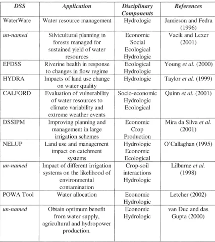
University, the Royal Forestry Department and departments from Chiang Mai, Maijo, and Kasetstart Universities. The Integrated Water Resource Assessment and Management (IWRAM) project was established to develop a Decision Support System for exploring options in water resources management. The DSS was developed to distinguish between different management scenarios and to allow for the exploration of trade-offs amongst them. A major challenge of the IWRAM project was to develop a modelling framework that includes the relevant biophysical, economic and socio-cultural components existing in the catchments (Jakeman et al., 1997). Reflecting this, the DSS was designed to provide stakeholders with a tool that, in addition to modelling hydrologic and erosional processes, incorporates local socio-cultural and econorruc realities. The primary objective of the project was to develop participatory and analytical procedures to allow stakeholders within the Ping Basin to identify and assess options for the sustainable development of rural catchments in Northern Thailand (Jakeman et al, 1997). Impacts of scenarios are distinguished using indicators of both biophysical and socio-economic outputs. The biophysical indicators may include quantity of streamflow at various nodes within the catchment or estimates of potential erosion from different soil or land unit classes, whilst economic indicators may include trends in the variability of agricultural production. Figure 1.1 shows the interactions between the components of the IWRAM Decision Support System.

(23)

biophysical relationships that are already hotly contested (Alford, 1992; Enters, 1995; Schmidt-Vogt, 1998).

I

Biophysictd Component • Flow and water quality

[image:23.600.138.540.139.399.2]

models • Cropmodel • Erosion model

... Climate

On-site and off-site I ~---~

~

costs of land use and I

erosion, benefits of / agriculture

,

I

/

.:

Economi.c Component • Economic Modelling of

Resource Management Units (RMU)

DECISION

SUPPORT

SYSTEM

- - - ->

_{Benefits and}

costs of options

\ \

\

\ Land Use Options \

\ \

\

Socio-cultural Component • RMU analysis

• Policy analysis • Scenario Generation

Figure 1.1. Interaction between the biophysical, economic and socio-cultural components and the IWRAM-DSS (adapted from Jakeman et al., 1997).

Details on the IWRAM-DSS can be found in Dietrich et al. (1999) and Letcher et al. (2002). The IWRAM project and its biophysical component were outlined in Jakeman et al. (1997) and Jakeman and Letcher (2001).

(24)

The study area considered for the development of the Biophysical Toolbox - and the IWRAM-DSS - is the Mae Chaem catchment, a 4000 km2 _{catchment in northern}

Thailand. Within the IWRAM project, four subcatchments of the Mae Chaem were focused upon. The development of the hydrologic component required a number of additional catchments for testing as the four subcatchments of interest in the IWRAM project were not gauged. Further details of the characteristics of the Mae Chaem catchment are provided in Chapter 2. A particular aim of the project was that the framework for evaluating water resources management be capable of being easily applied to catchments other than the Mae Chaem Catchment. Consequently, emphasis has been placed on using a modelling framework that allows the addition of required models or tools and removal or replacement of obsolete tools.

The thesis involves three major components of research:

• Implement an approach to estimate sheet erosion within the catchment. The approach implemented allows the development of indicators of potential erosion for the catchment in relation to rainfall and land cover scenarios.

• Develop a methodology for predicting streamflow response to land use or land cover changes in ungauged, or poorly gauged, catchments. Given limited data availability in northern Thailand a regionalisation approach for inferring hydrologic response in ungauged catchments was developed. This contributes to the understanding of hydrologic problems and water resource management in Thailand where catchments are frequently not instrumented at the scales required for impact assessment such as at village nodes. The method is tested for the gauged subcatchments within the Mae Chaem catchment in northern Thailand by comparing modelled and observed streamflow series.

(25)

The extent to which crop modelling is considered within this thesis is to explore the uncertainties within the model, particularly as they relate to inputs into the other models.

Emphasis is placed on developing and testing these individual components and exploring the issues involved in their integration within the Biophysical Toolbox of the DSS being developed within the IWRAM framework.

As the outcome of the IWRAM project is the development of a DSS, a number of limitations were placed on the modelling approaches. Firstly, the chosen approaches could not be too complicated or data intensive. Otherwise, this may have led to problems of model identifiability where parameters possess a large range of uncertainty (See Section 1.2.2.5). Even technical stakeholders within government departments may not have the expertise or time required to use a complicated DSS. The availability of data as well as other resources did not warrant the development of highly complicated modules. Secondly, the choice of an appropriate model for the crop, erosion, or hydrologic module was constrained by the availability of field and catchment data with which to drive the selected model and verify model behaviour. Additionally, the biophysical components of the DSS had to be integrated with social and economic modelling components (Letcher et al., 2002). The strength of the assumptions made in the socio-economic modelling did not warrant a detailed biophysical modelling approach. Overall, the aim has been to establish the directions and magnitudes of changes in indicators for given scenarios.

(26)

Chapter 1: Introduction

1.2 Environmental Modelling: Reconciling Issues in Modelling

the 'Real World'

6

The development of tools for exploring the assessment and management of environmental issues is increasingly being proposed as a means of assisting policy making. A disturbing trend has been the move towards the down-scaling of field based evaluations in favour of the use of such tools. Consequently, considerable work needs to be undertaken to verify the performance of modelling tools, in particular those, now becoming widespread, which attempt to explore multi-issue and multi-disciplinary problems. This section explores some issues in environmental modelling focusing on the issues relating to model construction, particularly in terms of natural complexity and spatial and temporal heterogeneities, before briefly reviewing recent work in integrated assessment (IA) and Decision Support Systems (DSS). No discussion is provided with regards to the requirements of integrated assessment. The review of DSS and IA is not intended as a comprehensive review of such tools. More comprehensive reviews are provided by Rizzoli and Young (1997) and Letcher (2002). McKinney et al. (1999) provides a discussion of integrated hydrologic-economic models and spatial decision support systems (SDSS).

Much of the discussion in Sections 1.2.1 and 1.2.2 is covered in more detail in Merritt et al. (2003c).

1.2.1 lssues of Data Availability, Complexity and Scale

(27)

factors need to be considered in order to choose the appropriate model for an application. These can be summarised as the suitability of the model to site conditions and data requirements, model complexity, the accuracy and validity of the model, model assumptions, spatial and temporal variation, components of the model and the objectives of the model user(s).

Jakeman et al. (1999) noted that the difficulties in environmental modelling can be characterised as problems of natural complexity, spatial heterogeneity and lack of available data. The complexity of natural systems is due to the differences in dimensions, temporal and spatial scales, and thresholds of water flow and sediment and nutrient transport through and within the media. Natural systems, from plot to catchment scale, tend to show a great deal of variation. Grayson and Moore (1993) noted that the scale at which uniformity is assumed in hydrologic models is generally greater than the scale at which directly measurable parameters are measured in the field, although smaller than shown by outflow hydrographs. Model predictions are thus subject to errors as a result of the inconsistency of scale between measured parameters and the way they are used in the model. Not only are there inconsistencies of scale between the measured parameters and their use in the model, there are often conflicts of scale between the various parameters themselves in the model. Batchelor et al. (1998) identified potential social and biophysical driving forces that drive a hydrologic system, which range in scale dependency from the farm level (e.g. family structure, soil type, vegetation distribution) to the subnational or regional scale (e.g. commodity prices, infrastructure development, annual rainfall and seasonality).

(28)

1.2.2 Model Types and Model Identification

The extent to which different modelling approaches can overcome some of the difficulties in modelling environmental issues is partly determined by the model type and the manner in which the system is represented.

Prior to discussing model types it is useful to raise the issues of model identification and over-parameterisation. Given limited data, most complex models require calibration, regardless of the model type. Most calibration techniques used for models of medium complexity are capable of finding only local optima at best. Spear ( 1995) noted that for large simulation models 'there is not a single point in the parameter space associated with good simulations, indeed there generally is not even a well-defined region in the sense of a compact region interior to the prior parameter space'. Identifying a unique 'best' parameter set in terms of goodness of fit is not likely. In general, simpler conceptual models have fewer problems with model identification than more complex models. However, reduction in problems associated with identifiability through simplification of models may come at the expense of goodness of fit to calibration data. More complex models are more likely to provide a better fit to calibration data. This does not necessarily extend to providing better predictions of future behaviour. The more linkages (i.e. the greater the model complexity) the more potential there is for error accumulation when a model is run in simulation mode compared with calibration mode (Croke and Jakeman, 2001 ).

(29)

used to describe erosion or sediment transport in the model. Examples of this are the so-called conceptual erosion modules that incorporate components of the empirical Universal Soil Loss Equation (USLE - Wischmeier and Smith, 1978) such as AGNPS (Young et al., 1989). Where the mix of modules is fairly even, a model is classified as a hybrid between two or more classes. In this thesis, an attempt to use consistent terminology for the crop, erosion, and hydrologic modelling components has led to the adoption of the classification of models into empirical, conceptual or physics based.

1.2.2.1 Empirical Models

Empirical models are generally the simplest model type, capable of being supported by coarse measurements. These models are often based on the analysis of catchment data using statistical techniques, and hence are suitable tools for the analysis of data within catchments. Most empirical models do not attempt to represent the physical processes involved. They tend to be catchment specific, applying only to the catchment for which they have been developed and often under the specific conditions existing within the site at that time. Often they ignore the heterogeneities of catchment inputs and characteristics, such as rainfall and soil types, and inherent non-linearities in the response of the system. The ability of empirical models to predict the effects of changes in catchment characteristics on water quality and sediment yields can therefore be limited. Empirical models also tend to be static, not being event responsive or responsive to antecedent conditions. Empirical hydrologic models or water quality models, for example, ignore the processes of rainfall-runoff in the catchment being modelled. Despite their obvious limitations, empirical models are frequently used in preference to more complex models as they can be implemented in data poor situations and are particularly useful as a first step in identifying sources of, for example, sediment and nutrient generation.

1.2.2.2 Conceptual Models

(30)

scale at which outputs are simulated, although this is not necessarily the case. Recent conceptual models tend to provide outputs in a spatially distributed manner. Although, conceptual models are based on important processes taking place, parameter values generally can not be measured due to the (usually) lumped nature of the model structure. Parameter values for conceptual models are generally obtained through calibration against observed data such as stream discharge and concentration measurements. Thus, these models may suffer from problems associated with the identifiability of their parameter values. In terms of complexity and consideration of processes, conceptual models provide a compromise between empirical and physics based models.

1.2.2.3 Physics Based Models

Physics based models are grounded on the solution of fundamental physical equations describing processes within the catchment. Standard equations used in such models are the equations of conservation of mass and momentum for flow and the equation of conservation of mass for sediment (e.g. Bennett, 1974).

Although the parameters used in physics based models are theoretically measurable, the large number of parameters involved and the heterogeneity of important characteristics within the catchment means that in practice these parameters must typically be calibrated against observed data. This creates additional uncertainty in parameter values. Like complex conceptual models, physics based models are prone to problems with the lack of identifiability of model parameters, and non-uniqueness of 'best fit' solutions can be expected. The fact that these models tend to have larger parameter and data requirements makes them particularly prone to issues of model identifiability if the model does need to be calibrated.

(31)

generally derived for use with continuous spatial and temporal data, but the data used in these models is often point source data taken to represent an entire grid cell within the catchment. Often there is little information to show whether many of the equations used in the models are valid beyond the small plot scale (Pickup and Marks, 2001). Additionally, there is often a lack of observed physical and biological data within catchments with which to drive these models. Hence, equations describing individual processes in physics based models are regularly subject to numerous assumptions that may not be relevant in many real world situations (Dunin, 1975).

Physics based models also tend to have greater data and computational requirements than other model types. The increased computational demands are greatest when ordinary or partial differential equations need to be solved on a discrete basis (Croke and Jakeman, 2001).

1.2.2.4 Distributed Versus Lumped Modelling

Another way to view the range of models is the way in which they represent the catchment or site to which the model is applied; that is, whether the model considers processes and parameters to be lumped or distributed. Traditionally, models have treated input parameters as lumped over the area of analysis. With increases in computing power over the last three decades, the distributed approach has become more feasible (e.g. ANSWERS - Beasley et al., 1980; TOPOG_IRM - Zhang et al., 1999). Distributed models reflect the spatial variability of processes and outputs within the catchment under analysis. As Leon et al. (2001) stated with respect to diffuse sources of pollutants, 'the difficulty in modelling non-point source is the problem of identifying and quantifying the loads as they are an aggregate of small contaminant inputs distributed through the catchment'. Thus, the authors argued, non-point source pollutant models require a distributed modelling approach. This attitude is reflected within the literature with an increase in the proportion of distributed modelling techniques presented.

(32)

distributed models with in-stream components, the outputs for each grid cell are then routed through the system to produce catchment scale outputs. Distributed models raise a number of issues, including increased data requirements and, perhaps more importantly, effects of grid resolution on model outputs. Input requirements potentially increase dramatically when each grid cell requires information. These models have often been linked with Geographical Information Systems (GIS). The issue of grid resolution on model outputs has been addressed for hydrologic modelling (e.g. Zhang and Montgomery, 1994; Quinn et al., 1995; Valeo and Moin, 2000) and sediment generation modelling (e.g. Schoorl et al., 2000).

A compromise between fully distributed methodologies and lumped models is provided by the semi-distributed models that disaggregate a catchment into a group of subcatchments or similar units over which the model is applied. An example of such an approach is the TOPMODEL hydrologic model (Beven and Kirkby, 1979), where an area is split into grid cells at which the topographic index,

z,

is calculated according to the equation

X

=

Zn( a/tan

/J)

(1.1)

where a is area and

fJ

is slope. All grid cells with the same value of the topographic index are assumed to behave in a hydrologically similar way, and this decreases both the number of computations and the data requirements for the model.

(33)

1.2.2.5 Selecting an Appropriate Model Structure

Obviously, these model types each serve their purpose and a particular model type can not categorically be considered more appropriate than others in all situations. Choice of a suitable model structure relies heavily on the function that the model needs to serve. Of particular importance in this thesis is that not only should the chosen models within the Biophysical Toolbox have adequate information available for use on their own, but that the inputs that one model provides to another be associated within some level of reliability. Some checks of the uncertainties associated with model outputs need to be in place before model outputs can be used as inputs to other models. Overly complicated models with large numbers of processes and parameters run the risk of the uncertainties associated with model inputs, and therefore outputs, clouding the performance of the whole toolbox. Within this thesis, emphasis is placed upon the links between model components and maintaining the balance between modules. As Parson (1996) stated with reference to Integrated Assessment, 'to gain a comprehensive view or highlight broad links . . . simple schematic representations must be used when richer ones are available'. This is equally applicable to the development of a toolbox such as that developed in this thesis.

1.2.3 Issues in Integrated Assessment of Land and Water Resources

(34)

authors stressed that 'integrated management must be the primary approach to addressing sustainable water resources'.

IA has a number of functions suitable for use as both policy-making (or guiding) and research tools. Risbey et al. ( 1996) identified that IA can be used as:

• a model building exercise

• a methodology for gaining insight over an array of environmental problems spanning a wide variety of spatial and temporal scales, and

• a process for providing an organising framework for conducting research.

Following on with the last point, a primary task within an IA framework is to identify key variables that are both relevant and measurable (Park and Seaton, 1996). Generally, IA has been aimed at developing models that attempt to integrate information by linking representations of the different components of natural and social systems in a computer model (Risbey et al. 1996). The extent to which this is achieved can be assessed using the example benchmarks for evaluation of research proposed by Janssen and Goldsworthy (1996). This involves:

• a completed diagnosis

• a functioning model that presents the problem situation

• availability of data to feed the model

• an inventory of possible solutions

• experimental solutions, and