Hydrodynamic instability in eccentric astrophysical discs

(1)

This is a repository copy of

Hydrodynamic instability in eccentric astrophysical discs

.

White Rose Research Online URL for this paper:

http://eprints.whiterose.ac.uk/108974/

Version: Accepted Version

Article:

Barker, AJ orcid.org/0000-0003-4397-7332 and Ogilvie, GI (2014) Hydrodynamic instability

in eccentric astrophysical discs. Monthly Notices of the Royal Astronomical Society, 445

(3). pp. 2637-2654. ISSN 0035-8711

https://doi.org/10.1093/mnras/stu1939

(c) 2014, Oxford University Press. This is an author produced version of a paper published

in Monthly Notices of the Royal Astronomical Society. Uploaded in accordance with the

publisher's self-archiving policy.

[email protected]

https://eprints.whiterose.ac.uk/

Reuse

Items deposited in White Rose Research Online are protected by copyright, with all rights reserved unless

indicated otherwise. They may be downloaded and/or printed for private study, or other acts as permitted by

national copyright laws. The publisher or other rights holders may allow further reproduction and re-use of

the full text version. This is indicated by the licence information on the White Rose Research Online record

for the item.

Takedown

If you consider content in White Rose Research Online to be in breach of UK law, please notify us by

(2)

Hydrodynamic instability in eccentric astrophysical discs

A. J. Barker

⋆

_{and G. I. Ogilvie}

Department of Applied Mathematics and Theoretical Physics, University of Cambridge, Centre for Mathematical Sciences, Wilberforce Road, Cambridge CB3 0WA, UK

23 September 2014

ABSTRACT

Eccentric Keplerian discs are believed to be unstable to three-dimensional hydro-dynamical instabilities driven by the time-dependence of fluid properties around an orbit. These instabilities could lead to small-scale turbulence, and ultimately modify the global disc properties. We use a local model of an eccentric disc, derived in a companion paper, to compute the nonlinear vertical (“breathing mode”) oscillations of the disc. We then analyse their linear stability to locally axisymmetric disturbances for any disc eccentricity and eccentricity gradient using a numerical Floquet method. In the limit of small departures from a circular reference orbit, the instability of an isothermal disc is explained analytically. We also study analytically the small-scale instability of an eccentric neutrally stratified polytropic disc with any polytropic in-dex using a WKB approximation. We find that eccentric discs are generically unstable to the parametric excitation of small-scale inertial waves. The nonlinear evolution of these instabilities should be studied in numerical simulations, where we expect them to lead to a decay of the disc eccentricity and eccentricity gradient as well as to induce additional transport and mixing. Our results highlight that it is essential to consider the three-dimensional structure of eccentric discs, and their resulting vertical oscilla-tory flows, in order to correctly capture their evolution.

Key words: accretion, accretion discs – planetary systems – hydrodynamics – waves – instabilities

1 INTRODUCTION

Astrophysical discs with eccentric orbits have been proposed to explain a number of astrophysical observations. They are thought to explain the superhump phenomenon in SU UMa stars (Whitehurst 1988; Lubow 1991a; Smith et al. 2007), the spectral variability of rapidly rotating Be stars (Okazaki 1991; Papaloizou et al. 1992; Ogilvie 2008) and, in the case of a collisionless disc of stars, the visible structure of the nu-cleus of the galaxy M31 (Tremaine 1995; Peiris & Tremaine 2003). In addition, the orbital evolution of a newly born planet due to its tidal interaction with the protoplanetary disc is intricately coupled with the evolution of eccentric modes in the disc. The excitation and damping of these modes may have played a role in the early evolution of plan-etary eccentricities (Papaloizou et al. 2001; Papaloizou 2002; Goldreich & Sari 2003; Kley & Dirksen 2006; D’Angelo et al. 2006; Bitsch et al. 2013).

Eccentric modes in Keplerian discs are slowly precessing modes with azimuthal wavenumber m = 1 (e.g. Tremaine 2001; Papaloizou 2002) that vary on a length scale compa-rable with the radius of the disc. Because of their global

⋆ _{Email address: [email protected]}

extent they are usually thought to be extremely long-lived. However, a gaseous eccentric disc may be unstable to hy-drodynamic instabilities, and these may limit the lifetime of the eccentricity.

(3)

the disc eccentricity and could limit the eccentricities of ob-servable discs. In this paper we use the local model to study the linear stability of an eccentric disc.

Papaloizou (2005a) was the first to study the hydro-dynamic instability of eccentric Keplerian discs, motivated by the earlier work of Goodman (1993) and Lubow et al. (1993) for tidally deformed discs (which have m = 2). He found that eccentric discs were unstable to a parametric in-stability that took the form of resonantly excited inertial waves. Their nonlinear evolution in a global disc model was subsequently studied in Papaloizou (2005b), where they led to small-scale subsonic turbulence (or wave activity) and to a gradual decay of the disc eccentricity. The pioneering calculations of Papaloizou (2005a) were limited to studying the three-dimensional stability of a uniformly eccentric disc without vertical structure. In this paper we use the newly derived local model to study the local linear stability of discs with any eccentricity and eccentricity gradient, taking into account the vertical structure of the disc in full.

The structure of this paper is as follows. In§2 we write down the equations describing fluid dynamics within the lo-cal model derived in OB14, and describe the resulting ver-tical oscillatory flows in the disc. We set up the local linear stability analysis of an eccentric disc in§3, analyse this sys-tem numerically in§4, and end with a discussion and con-clusion. Detailed analytical understanding of the instability is relegated to Appendices B to D.

2 LOCAL MODEL AND LAMINAR FLOWS

The basic equations describing ideal isothermal hydrody-namics within the local model of a coplanar eccentric Ke-plerian disc are summarised in this section. The properties of an eccentric orbit in a coplanar Keplerian disc can be de-scribed by the following parameters: the semi-latus rectum

λ(related to the semi-major axisabyλ=a(1−e2_{)), the}

ec-centricitye(λ), and the longitude of pericentreω(λ). When formulated in dimensionless terms, the local model is inde-pendent ofλ, but does depend on the local eccentricitye, as well as the dimensionless local gradients in the eccentricity

λe′ _≡_λ_d_e/_d_λ_and _eλω′ _≡_eλ_d_ω/_d_λ_{, where the latter may} be thought of as a measure of the twist in the disc. These may be combined into the complex eccentricity E = eeiω and eccentricity gradientλE′₌_λ_d_E/_d_λ_.

The local model derived in OB14 is valid for a thin disc with ǫ = H/r ≪ 1 and describes fluid dynamics in a small patch of the disc centred around a reference orbit at the mid-plane with orbital coordinates (λ0, ϕ(t),0).

Ow-ing to the geometry of an eccentric orbit, it is convenient to adopt (in general) non-orthogonal coordinates (ξ, η, ζ), whereξ=λ−λ0 is a quasi-radial coordinate,η=φ−ϕ(t)

is an angular coordinate andζ=zis the usual vertical coor-dinate. The coordinates (ξ, λ0η, ζ) are equivalent to

Carte-sian coordinates when the orbit is circular – in this case the system of equations that we will list below reduces to the standard shearing box commonly used to study the dynam-ics of astrophysical discs.

We define the contravariant velocity components (vξ_{, v}η_{, v}ζ_{) and the enthalpy} _h_{, where the latter is defined} by

h=c2slnρ+ const, (1)

for an isothermal ideal gas with sound speedcs, in which the pressurepis related to the densityρbyp=c2sρ.

The linear stability of an eccentric disc to a general non-axisymmetric disturbance is complicated considerably by the presence of Keplerian shear, so we consider locally axisymmetric motions in this work. The resulting (inviscid) equations in the local model are (Eq. 80–83 in OB14)

Dvξ+ 2ΓλλφΩvξ+ 2Γφφλ Ωvη=−gλλ∂ξh, (2) Dvη+ (∂λΩ + 2ΓφλφΩ)v

ξ_{+ (}_∂

φΩ + 2ΓφφφΩ)v

η₌ ₍₃₎

−gλφ∂ξh, Dvζ =−Φ2ζ−∂ζh, (4)

Dh=−c2s

∆ +∂ξvξ+∂ζvζ

, (5)

where

D≡∂t+vξ∂ξ+vζ∂ζ, (6)

is the Lagrangian derivative. We have evaluated the orbital angular velocity Ω and its derivatives, as well as the met-ric and connection coefficients, at a reference point in the mid-plane of the disc (λ0, ϕ(t),0), so that these become

pe-riodic functions of time only. The orbital velocity divergence is written as ∆, which is nonzero when the disc has an ec-centricity gradient (see OB14 and Appendix A).

The gravitational potential expanded about the mid-plane takes the form (withζ=O(ǫ))

Φ = Φ0+

1 2ζ

2_Φ

2+O(ζ4), (7)

where Φ0=−GM/Rand Φ2=GM/R3, andRis the

cylin-drical radius. The periodic variation of Φ2around an orbit is

responsible for driving vertical oscillatory flows in the disc. These (nonlinear) oscillations can be obtained by looking for simple solutions of Eqs. 2–5 of the form

vξ=vη= 0, vζ=w(t)ζ, h=f(t)−1₂ζ2g(t), (8)

which satisfy the following ODEs:

dtw+w2=−Φ2+g, (9)

dtf=−c2s(∆ +w), (10) dtg=−2wg. (11)

The laminar flow functionsf andg=c2sH−2 (whereH(t) is the Gaussian scaleheight of the isothermal disc), together define the surface density of the disc

Σ∝e f c2

sc_sg− 1 2 _∝_e

f c2

sH, (12)

satisfying

dtΣ =−∆Σ, (13)

so that the surface density is constant around an elliptical orbit when ∆ = 0, but varies if ∆6= 0.

Periodic solutions of Eqs. 9–11 can be computed nu-merically using a shooting method. Several examples have been plotted in OB14. Note thatλe′ andeλω′play no role in determining g and w in the isothermal approximation (although the enthalpy at the mid-planef does depend on ∆).

c

(4)

3 LINEAR STABILITY OF ECCENTRIC DISCS

3.1 Linearised axisymmetric perturbation equations

We consider small perturbations to the orbital motion and vertical laminar flows of the form Reˆvξ(ζ, t)eikξξ_{, and so} on for other variables, wherekξ is a quasi-radial wavenum-ber. We subsequently drop the hat on the perturbations for

clarity. We choose units such that Ω0 =

GM

λ3 0

1 2

= 1 and

cs = 1, therefore the disc thickness would take a constant valueH=g−1

2 = 1 for a circular disc.

We note that it is much simpler to use the true anomaly

θ as a variable rather than t, and that the corresponding rates of change are related by∂t = Ω∂θ = (1 +ecosθ)2∂θ. This variable is used as a “time-like” variable, and is con-tinuous and monotonically increasing, not restricted to the range [0,2π]. We further definec≡cosθ ands≡sinθ. The resulting linearised perturbation equations are

Ω∂θvξ+wζ∂ζvξ+ 2ΓλλφΩvξ+ 2ΓλφφΩvη=−igλλkξh, (14)

Ω∂θvη+wζ∂ζvη+

∂λΩ + ΓφλφΩ

vξ

+∂φΩ + 2Γφφφ

vη=−igλφkξh, (15)

Ω∂θvζ+wζ∂ζvζ+wvζ=−∂ζh, (16) Ω∂θh+wζ∂ζh−gζvζ =−ikξvξ−∂ζvζ. (17)

The coefficients are periodic functions ofθ with period 2π, which we list in Appendix A. A statement of conservation of energy for the perturbations can be derived at this stage, which we present in Appendix C – this is used to analyse the energetics of the resulting instabilities.

The vertical structure of waves in a circular isothermal disc take the form of Hermite polynomials inζ(e.g. Okazaki et al. 1987; Ogilvie & Latter 2013). These have the property that the energy density of the perturbations tends to zero at large distances from the mid-plane. In the eccentric case, Eqs. 14–17 also have exact solutions that are polynomials in ζ. These solutions can be represented as finite sums of (probabilist’s) Hermite polynomials:

vξ =

N X

n=0

uξn(θ)Hen(ζ), (18)

vη =

N X

n=0

λ−1uηn(θ)Hen(ζ), (19)

vζ =

N X

n=1

uζn(θ)Hen−1(ζ), (20)

h =

N X

n=0

hn(θ)Hen(ζ), (21)

where N is the vertical mode number. The factor of λ−1

ensures thatuηnhas units of velocity. Note that

dζHen(ζ) = nHen−1(ζ), (22)

ζHen(ζ) = Hen+1(ζ) +nHen−1(ζ). (23)

The resulting ODEs are

(1 +ec)2dθw+w2=−Φ2+g, (24)

(1 +ec)2dθf=−(∆ +w), (25) (1 +ec)2dθg=−2wg, (26)

for the laminar flows, and

(1 +ec)2dθuξn+w h

nuξn+ (n+ 1)(n+ 2)uξn+2

i (27)

+2ΓλλφΩuξn+ 2λ−1ΓλφφΩuηn=−igλλkξhn, (1 +ec)2dθuηn+w

nuηn+ (n+ 1)(n+ 2)uηn+2

(28) +uξnλ∂λΩ + 2λΓ_λφφ Ωuξn+ ΓφφφΩu

η

n=−iλgλφkξhn, (1 +ec)2dθuζn+w

h

(n−1)uζn+n(n+ 1)uζn+2

i (29)

+wuζn=−nhn,

(1 +ec)2dθhn+w[nhn+ (n+ 1)(n+ 2)hn+2] (30)

−(g−1)huζn+ (n+ 1)uζn+2

i

=−ikξuξn+uζn,

for the linear perturbations. Eq. 29 is valid for 16n 6N

and the other three are valid for 06 n 6N. We have set

uξn= 0 etc forn > N by considering polynomial solutions. This is the system of equations that we will solve to de-termine the linear stability of an eccentric disc to locally axisymmetric perturbations. Note that vertical hydrostatic equilibrium corresponds tog = H−2 _{= 1, which does not}

hold in an eccentric disc, in general. Also, note that there are three dimensionless parameters that define the local or-bital properties of the eccentric disc:e, λe′_{, eλω}′_.

For a given vertical mode numberN, the set of 4N−1 equations given by Eqs. 27–30 are analysed numerically us-ing a Floquet method. This method is appropriate since the coefficients are periodic functions ofθ. First, the monodromy matrix of linearly independent solutions is constructed by integrating the ODEs over one period (in the process the laminar flows are also computed) for initial conditions such that all variables except one are set to zero. The eigenvalues of the monodromy matrix allow us to obtain the complex growth rates of the instability. See Ogilvie & Latter (2013) for details of a similar approach used to study the instabil-ities of a warped disc. We have verified that we obtain the correct linear dispersion relation for a circular disc, and we will illustrate in§4 that our numerically computed growth rates are in excellent agreement with the analytical predic-tions presented in Appendix B.

The vertical oscillations of the disc couple components with differentn whene 6= 0. However, these only couple a componentn with a componentm=n+ 2, and there are no additional couplings to components withm < n. These are then “one-way” couplings, for which components with

m < nare slaved to the maximum n. The growth rate of

(5)

3.2 Linear axisymmetric waves in a circular disc

Whene=λe′ =eλω′ =w=g−1 = 0, the above system reduces to

dθuξn−2Ωunη =−ikξhn, (31)

dθuηn+ 1 2Ωu

ξ

n= 0, (32)

dθuζn=−nhn, (33) dθhn=−ikξuξn+uζn. (34)

Looking for solutions proportional to e−iωθ_{, we obtain the} ideal dispersion relation describing axisymmetric waves in a circular isothermal Keplerian disc:

(−ω2+n)(−ω2+ 1)−k2ξω2= 0. (35)

The low frequency branch for n 6= 0 corresponds to iner-tial waves. A pair of ineriner-tial waves with ω = ±12 (which

occurs whenkξ = 1₂ p

3(4n−1)) can be coupled to give 1, which is the frequency at which the geometrical coefficients in Eqs. 27–30 are modulated. For a given range ofkξ these resonant waves are fully captured by considering a finite range of vertical mode numbers. These are the waves that become unstable in an eccentric disc, as we will illustrate in the next section.

4 NUMERICAL CALCULATIONS

In a disc with nonzero eccentricity or eccentricity gradient the coefficients in Eqs. 27–30 become 2π-periodic functions ofθ. The periodic variation in the eccentric orbital motion of the gas around an orbit, together with the associated ver-tical oscillation of the disc, drive a parametric instability consisting of pairs of inertial waves. In the local model, the eccentric orbital motion has radial and vertical wavenum-bers of 0 and a frequency of 1 (i.e. the orbital frequency). For small departures from circularity, an instability is driven by a parametric resonance between the eccentric (and ver-tical) oscillation of the fluid around an orbit and a pair of inertial waves withω=±1/2 with the same radial and ver-tical wavenumbers. These waves propagate radially in oppo-site directions, and their superposition is a standing wave. These are coupled in an eccentric disc because their frequen-cies differ by 1. When the departure from circularity is not small (or if viscosity is included), there is a frequency band of instability around exact resonance whose width increases with the eccentricity. The instability of a disc with an eccen-tricity gradient is found to take the same form, as we will illustrate below. This instability is explained in detail in Ap-pendix B, where we analytically compute the growth rates at exact resonance. We have also analysed the sources of en-ergy driving the instability, which we present in Appendix C.

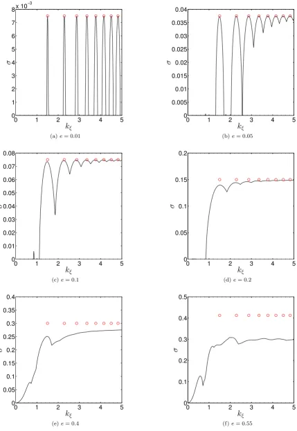
4.1 Uniformly eccentric disc

We first illustrate the instability of a uniformly eccentric disc, withλe′₌_λω′_{= 0. In Fig. 1, we plot the growth rate} of the fastest growing mode from our numerical calculations as a function of the radial wavenumberkξfor variouse. We have also plotted our analytical predictions from Appendix B for the growth rate (σ) at exact resonance as red circles,

10−2 10−1 100

10−3 10−2 10−1 100

σ

m

a

x

[image:5.595.329.519.47.236.2]

e

Figure 3.Maximum growth rate of the instability (forkξ∈[0,5])

as a function ofefor a uniformly eccentric disc (using units such that GM/λ3

0

12 _{= 1). The numerical results are plotted as blue}

circles, and were computed up toN = 12, which was found to be sufficient to obtain the fastest growing mode in all cases. The black dashed line is the theoretical prediction for smalle,σ = 3e/4.

where σ= 3e/4 independent of kξ when e ≪1. For small

e, instability occurs in discrete wavenumber bands centred on certain values ofkξ, which merge askξ → ∞. The first peak represents a pair of inertial waves withn= 1, there-forekξ= 3/2. The subsequent peaks represent inertial waves with sequentially increasingnin such a way that the waves have ω= ±1

2. As e is increased, the instability bands

be-come wider and merge, and their centres are shifted slightly from the analytical prediction. There is an additional peak at small kξ below the first instability band whose growth rate isO(e2_{); this instability is also found to have an}

iner-tial wave character. Fore&0.4, there is instability for any

kξ>0.

We illustrate the velocity field for one representative unstable mode whene= 0.01 in the (ξ, ζ)-plane in Fig. 2 – the velocity componentsuξ _and_uζ _{have been multiplied by}

ρ1/2to show the wave energy at four different phases around an orbit. This mode is a standing wave, whose amplitude is modulated in such a way to extract energy from the orbital flow and the vertical oscillation of the disc. The dominant contribution comes from the vertical oscillation of the disc, arising from a term Re−w|uζ_|2 _{in the energy equation,}

which has net contribution∝ −R02πsinθ(2−2 sinθ)dθ= 2π

(this is shown in detail in Appendix C). The mode has its maximum magnitude of vertical velocity at the phaseθ = 3π/2, at which−whas its maximum, therefore it can extract energy from the vertical oscillation most efficiently at this phase.

In Fig. 3 we plot the growth rate of the fastest growing mode maximised overkξin the rangekξ∈[0,5] as a function ofe. This range inkξ was chosen to limit to the computa-tional cost of a wide parameter search, and was found to be sufficient to capture the fastest growing mode in all cases. The numerical results are shown as blue circles and the

ana-c

_ξ

[image:6.595.74.504.44.668.2]

(f)e= 0.55

Figure 1.Instability of a uniformly eccentric disc withλe′₌_λω′_{= 0. The growth rate of the fastest growing mode (using units such} that GM/λ3

0

12 _{= 1) is plotted as a function of}_k

ξ for variouse. The red circles show the analytical prediction from Appendix B at

exact resonance, which is valid whene≪1. The numerical calculations were performed with vertical mode numbers up toN= 12, which was sufficient to obtain the fastest growing mode in all cases, and involved calculations at 400 uniformly distributed values ofkξ∈[0,5].

[image:7.595.76.500.55.461.2]

(d)θ= 3π/2

Figure 2. Illustration of the velocity field (multiplied by√ρto show the localisation of wave energy near to the mid-plane) of the n= 1 unstable mode at exact resonance whene= 0.01 for four different phases around an orbit. This is a standing mode composed of a superposition of travelling inertial waves propagating in opposite directions radially. The arrows have the same scale in each panel. When the “meridional” velocity perturbations vanish atθ= π₂, the azimuthal velocity perturbation is nonzero. The amplitude of the vertical velocity is correlated with the orbital motion in such a way to extract energy from the vertical oscillation of the disc, and is maximum atθ=3π

2, where−whas its maximum. Atθ= 2π, the mode returns to its form atθ= 0 but is slightly amplified and reversed in sign since its period is 4π.

lytical prediction is shown as a black dashed line with slope 3e/4. The small-e analytical prediction for the growth rate at exact resonance correctly captures the instability until

e & 0.4, above which the numerically determined growth rate is found to deviate. The peak growth rate is no longer independent ofkξ whene6≪1 (see Fig. 1).

The laminar flows were found to have quite extreme be-haviour fore&0.4 or so, with an asymmetric character such that there are strong compressions occurring very close to pericentre (OB14). That these laminar flows differ from sim-ple sinusoidal behaviour for moderately large eccentricities could reduce their ability to excite inertial waves, and might explain why the growth rate is smaller than would be pre-dicted from a simple extrapolation of the small-ebehaviour

fore& 0.4. Nevertheless, the growth rate in these cases is still large enough for the instability to be dynamically im-portant within a few orbits. For moderatee, instability is possible for anykξ>0.

Note that the maximum growth rate for the local in-stability in a uniformly eccentric isothermal disc is much stronger than the corresponding growth rate obtained by Pa-paloizou (2005a). He found that in a cylindrical disc model (without vertical structure), σ = 3e/16 in the limit that

kξ, n → ∞. The difference between these follows from our inclusion of the laminar vertical oscillation of the disc, which provides an additional periodic forcing, and an additional free energy source. The vertical disc oscillations are thus able to amplify the growth rate of the instabilities. We have

c

(8)

10−2 10−1 100 10−3

10−2 10−1 100

σ

m

a

x

[image:8.595.68.257.48.238.2]

λ

e

′

Figure 5. Maximum growth rate of the instability (for kξ ∈

[0,5]) as a function of|λe′_|_when_e_{= 0 (using units such that} GM/λ3

0

12 _{= 1). The numerical results are plotted as blue}

cir-cles, and were computed up toN = 12, which was found to be sufficient to obtain the fastest growing mode in all cases. The black dashed line is the theoretical prediction for small |λe′_|_, σmax= 3|λe′|/16.

confirmed that we obtain the analytical prediction of Pa-paloizou (2005a) if we artificially neglect the laminar flows by choosingw=g−1 = 0 (see Appendix B). This highlights the importance of considering the three-dimensional struc-ture of an eccentric disc to correctly capstruc-ture the instability.

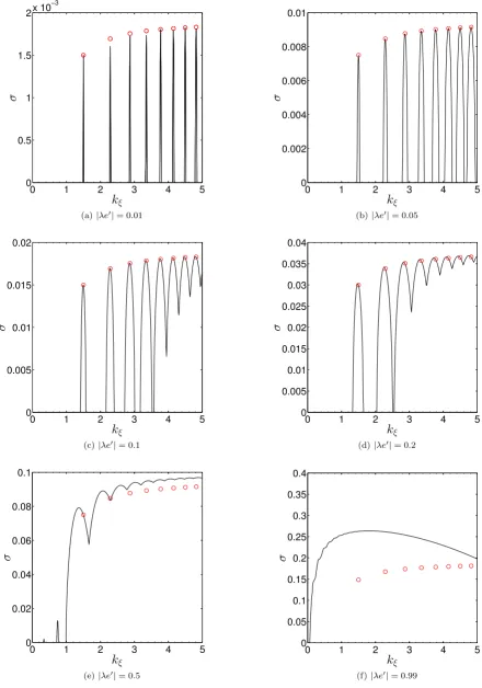
4.2 Circular reference orbit with nonzero eccentricity gradient

The next case to consider turns out in fact to be the simplest: the instability of a disc that is locally circular but has a nonzero eccentricity gradient. In this case, w =g−1 = 0 for an isothermal disc, so that the vertical laminar flows are no longer present, and there are no corresponding couplings between different n in Eqs. 27–30. An instability is driven by the periodic variation of the orbital motion of the gas on orbits that neighbour our reference circular orbit. This is analysed in Appendix B, and is found to have the same character as the instability described in§4.1.

In Fig. 4 we plot the growth rate of the fastest growing mode from our numerical calculations as a function of the radial wavenumberkξfor various|λe′|. We have also plotted our analytical predictions from Appendix B for the growth rate at exact resonance as red circles, where for small|λe′_|_,

σ = 3|λe′|/16 for large kξ, n. In this case the instability is somewhat weaker than that for a uniformly eccentric disc because the additional energy source provided by the verti-cal oscillations of the disc is absent. This means that for the smallest|λe′_|_{that we have considered, the instability bands} are very narrow (in the first panel, exact resonance is not captured by our distribution of points inkξ). However, for large|λe′|, instability is possible for anykξ>0. Note that non-intersecting orbits must have |λe′_| _< _{1 (if this is}

vio-lated, the instability that we have described will no longer be relevant, since the flow will develop shocks).

In Fig. 5 we plot the growth rate of the fastest growing mode maximised overkξ in the rangekξ ∈[0,5] as a func-tion of|λe′_|_{. The numerically determined values are shown} as blue circles and the black dashed line shows the small-|λe′|

analytical prediction askξ, n → ∞. The analytical predic-tion works well until |λe′_{| ∼} _{1, near to which the growth} rate is slightly amplified over the small-|λe′_|_prediction.

4.3 General eccentric disc

We will now describe the instability for the more general configuration of an eccentric disc with a nonzero eccentricity gradient. The requirement for orbits to not intersect is

e−λe′2+e2(λω′)2<1. (36)

If this is violated, we expect shocks to form, and they are likely to dominate the evolution of the disc. We compute the maximum growth rate of the instability and plot its contours on the (λe′−e, eλω′)-plane for several values of ein Fig. 6 – this plane was chosen since the requirement for orbits to be non-intersecting is represented as the region inside the unit circle. This figure illustrates that we have instability over most of the (e, λe′_{, λω}′_{) parameter space, and that the} growth rate is generally larger when we have larger eccentric-ities, as well as larger eccentricity gradients. The analytical prediction for this general case for small departures from a circular reference orbit is presented in Appendix B. We find that the instability of an eccentric disc is stronger for larger1 _e₊_λe′_{. Note, however, that there is a region where} the instability is weak, centred onλω′_{= 0. For large}_n_the growth rate is zero whenλe′₌₋₄_e_{for small}_e_{(though the} growth rate is not exactly zero for any finite n), which is predicted by the analysis in Appendix B (departures from this prediction in Fig. 6 are apparent for larger e, where this region moves further to the left of the allowed param-eter space). For those particular choices of paramparam-eters, the coupling between the eccentric disc motion and the inertial waves is weak. However, instability is possible over nearly all of the parameter space for an eccentric disc.

For the case e = 0, which was described in §4.2, the only relevant parameter describing the orbit isλe′_{. In this} case, if we were to plot this on Fig. 6, the contours would be perfect circles centred on the origin, with the growth rate shown in Fig. 5. As e is increased, the growth rate con-tours begin to differ from circles and when e & 0.4, they become increasingly independent ofλω′ i.e. they are bet-ter approximated by vertical lines. This presumably results from the increasingly non-sinusoidal behaviour of the lam-inar flow solutions, which become more strongly localised near pericentre for moderately largee. Therefore they may not be as efficient at exciting inertial waves.

Fig. 6 illustrates that instabilities growing on a dynam-ical timescale are possible for an orbit with any eccentricity considered, as long as the eccentricity gradient is sufficiently

(9)

_ξ

[image:9.595.65.506.46.675.2]

(f)|λe′_|_{= 0}_.₉₉

Figure 4.Instability in the case of a circular reference orbit withe= 0 and a nonzero eccentricity gradient. The growth rate of the fastest growing mode (using units such that GM/λ3

0

1₂

55

−1 −0.5 0 0.5 1

−1 −0.8 −0.6 −0.4 −0.2 0 0.2 0.4 0.6 0.8 1

[image:10.595.53.518.40.595.2]

0.2 0.3 0.4 0.5 0.6 0.7 0.8 0.9

Figure 6. Growth rate of the instability (using units such that GM/λ3 0

1₂

= 1) maximised over kξ ∈ [0,5] for a general eccentric

(11)

large. This also shows that the instability of an eccentric disc is widespread.

5 NEUTRALLY STRATIFIED POLYTROPIC

DISCS: DEPENDENCE ON THE ADIABATIC INDEX

The results presented in §4 were obtained by assuming an isothermal relation, which is the most compressible model that we can adopt. Given that the compressibility of the disc plays an important role in driving the laminar vertical oscil-lations, and that the presence of these oscillations was found to significantly amplify the growth rate of the instability, it is important to determine how these results depend on the adiabatic index. In this section we describe our analytical re-sults for a neutrally stratified polytropic disc which behaves adiabatically withp ∝ργ_{, where} _γ _{= 1 + 1}_/n

p, andnp is the polytropic index. Realistic discs are expected to have

γ ≈1.4−1.7. We neglect any possible stable (or unstable) vertical stratification since this requires the eigenfunctions to be localised near to the mid-plane of the disc, and this would complicate the analysis.

In Appendix D we present the analytical theory describ-ing the locally axisymmetric instability of an eccentric disc using a WKB approximation, in which the radial and verti-cal wavelengths of the unstable mode are taken to be much smaller than the disc thickness. Looking for such small-scale instabilities allows us to treat the unstable modes locally as plane waves, which avoids the complication that there are no analytically computable eigenmodes for the circular polytropic disc, unlike the isothermal disc considered so far. The WKB theory in Appendix D extends the calculations of Papaloizou (2005a) to include the vertical structure of the disc, and to allow for any eccentricity gradient and adiabatic index (for a neutrally stratified disc).

The instability is found to take the same form for any

γ, and involves the excitation of pairs of inertial waves with

ω=±1/2 that form a standing wave. However, the growth rate of the instability is found to depend onγ. In particular, the instability for a uniformly eccentric disc has a growth rate

σ= 3

16

1 +3

γ

e, (37)

which is strongest for an isothermal disc (γ = 1 leads to 3e/4) and reduces to 3e/16 for an incompressible disc (γ→ ∞). An incompressible disc does not exhibit vertical laminar oscillations in this case, so the instability is driven purely by the periodic variation of the eccentric orbital motion around an orbit. Hence the agreement with the growth rate obtained by Papaloizou (2005a). This demonstrates once again that the vertical laminar flows play an important role in driving instabilities in an eccentric disc. Note that the growth rate is significantly amplified over the incompressible limit for any realistic γ. For example, σ = 21e/40 ≈ 0.525e when

γ = 5

3, which is appropriate for a disc consisting of ionised

hydrogen.

Similarly, if we consider the instability of a circular ref-erence orbit with a nonzero eccentricity gradient, we obtain

σ= 3

16γ|λe

′

|, (38)

which is strongest for an isothermal disc (3|λe′_|_/_{16), and} vanishes entirely in the incompressible limit.

The more general configuration of an eccentric disc with a nonzero eccentricity gradient is presented in Appendix D.

6 DISCUSSION

The local instability that we have analysed in this paper oc-curs whenever an astrophysical disc becomes eccentric. As-suming a simpleα-prescription for the turbulence in a Keple-rian disc, we can simply estimate to what degree a departure from circularity is required for the instability to grow in the presence of viscosity. The viscous damping rate of a mode with radial wavenumberkξ and vertical mode numbernis approximately2_α₍_k2

ξ+n), whereαis the viscosity coefficient. For a uniformly eccentric disc, we requiree&0.04(α/10−2₎

for the largest wavelength (n = 1, kξ = 3/2) instability to occur. Similarly, for a circular reference orbit with a nonzero eccentricity gradient, we require |λe′| & 0.17(α/10−2) for instability. Note, however, that instability is strongest for a combination of eccentricity and eccentricity gradient, there-fore instability may be possible even if these criteria are not satisfied. In addition, it is unclear whether the interaction of this instability with the turbulence that drives accretion in the disc can be modelled with a simpleα-viscosity prescrip-tion. Nevertheless, we conclude that instability is possible in a sufficiently eccentric disc for typical values of αthought to be relevant for circumstellar discs.

Another aspect is that the local instability involves the coupling of pairs of inertial waves that propagate radially in opposite directions in the disc to form a local standing wave. If the disc eccentricity or its gradient is localised to some region of the disc of radial extent D (the “interac-tion region”), the instability will only cause disturbances to reach large amplitudes if the waves spend enough time in that region to be sufficiently amplified. We expect the in-stability to be important if the growth time is shorter than the wave crossing time over this region (unless the waves can reflect from radial boundaries and re-enter the interac-tion region), which is approximatelyσ−1_._D/c

g, where the group velocity of an inertial wave is cg ∼ω/kξ. This sug-gests thatkξ &O((eD)−1) is required for the instability to amplify disturbances to large amplitudes, so that a small interaction region or a weak eccentricity will preferentially excite small-scale disturbances, which may be more difficult to observe in simulations, or be more easily damped by vis-cosity (this simplistic argument neglects the presence of an eccentricity gradient).

Previous grid-based hydrodynamical simulations of disc-companion tidal interactions have observed the gen-eration of local eccentricity and eccentricity gradients in the disc (e.g. Papaloizou et al. 2001; Kley & Dirksen 2006; D’Angelo et al. 2006; Kley et al. 2008; Marzari et al. 2012). However, the instabilities that we have described in this pa-per have never been observed previously3_{. This is partly}

be-2 _{The viscous linearised equations for the instabilities in a warped} disc were studied more carefully in Ogilvie & Latter 2013. 3 _{Except by Papaloizou (2005b), who performed a set of global} simulations specifically designed to study them for the specific case of a cylindrical disc (lacking vertical structure).

c

(12)

cause most of the existing simulations are two-dimensional, therefore they would be unable to capture the instability. In addition, these simulations would also incorrectly neglect the vertical laminar oscillations of an eccentric disc. The limited three-dimensional simulations that have been per-formed thus far (e.g. Bitsch et al. 2013) necessarily have limited spatial resolution (or too large a physical or numer-ical viscosity), so they may have been unable to capture the instability4. In addition, the instability may be too weak to be observed during the limited duration of some simula-tions, particularly when the disc eccentricity or eccentricity gradients do not attain large values.

In a similar way, global SPH simulations of eccen-tric discs in superhump binaries are either two-dimensional (Whitehurst 1988; Lubow 1991b), or they do not have suffi-cient spatial resolution to be able to capture these instabili-ties (Smith et al. 2007). Previous simulations have captured the exponential growth of eccentricity due to the tidal insta-bility of Whitehurst (1988) and Lubow (1991a), but they do not identify a mechanism of saturation for the instability. The instabilities that we have analysed in this paper may provide such a mechanism, because their growth rates are an increasing function of the eccentricity.

These instabilities may play a role in modifying the ec-centricities of planets undergoing tidal interactions with the protoplanetary disc. Secular interactions between the plan-ets and the disc will redistribute the angular momentum deficit between the various components, leading to oscilla-tions in the disc and planet eccentricities (e.g. Papaloizou et al. 2001; Papaloizou 2002; Goldreich & Sari 2003). When parts of the disc become eccentric, we speculate that the instabilities analysed here would lead to a decay of the disc eccentricity and eccentricity gradient (this behaviour was observed by Papaloizou 2005b). These instabilities would therefore reduce the angular momentum deficit of the sys-tem, and provide a mechanism for damping the eccentricities of the planets due to their secular coupling with the disc. To determine the efficiency of this damping process, nonlinear calculations are required, which we defer to future work.

7 CONCLUSIONS

In this paper we have studied the hydrodynamic stability of eccentric Keplerian discs. We have utilised a local model similar to the conventional shearing box, which we derived in a companion paper (OB14), to compute the vertical os-cillations of the eccentric disc, and to analyse their result-ing instabilities usresult-ing a numerical Floquet method. We have obtained detailed analytical understanding of the instabil-ity for isothermal discs (Appendices B and C), as well as for

4 _{The simulations in Bitsch et al. (2013) of an isothermal} verti-cally structured disc haveα= 0.005. The eccentricity of the disc attains values of approximatelye∼0.3 and|λe′_{| ∼} ₀_._{5, so the} largest wavelength instability can in principle be excited. How-ever, the radial extent of the region of moderate disc eccentricity is.1, so the most strongly excited waves will have smaller ra-dial wavelengths, withkξ &6, n&10, which will most likely be

damped by the viscosity adopted. Hence it is not surprising that this instability is not observed in their simulations.

polytropic discs with any polytropic index using a WKB ap-proximation (Appendix D), for any weak local eccentricity and eccentricity gradient. This work considerably extends the pioneering calculations of Papaloizou (2005a), who was the first to identify these instabilities for the specific case of a uniformly eccentric cylindrical disc.

We have highlighted the importance of considering three-dimensional effects and the disc vertical structure in order to understand the evolution of eccentric discs. This arises because vertical oscillations of the disc are driven by the periodic variation in the vertical gravitational accelera-tion around an eccentric orbit (identified by Ogilvie 2001). These oscillations provide an additional free energy source, and an additional periodic driving, of small-scale inertial waves. Instabilities with dynamically relevant growth rates are found in a disc with a sufficiently large local eccentric-ity or eccentriceccentric-ity gradient. Two-dimensional calculations would be unable to capture either of these effects, and are unlikely to correctly describe the evolution of eccentric discs. Disc-planet interactions can generate local disc eccen-tricity and ecceneccen-tricity gradients (Papaloizou et al. 2001; Kley & Dirksen 2006; D’Angelo et al. 2006; Bitsch et al. 2013). The secular interaction of planets with eccentric disc modes leads to an exchange of eccentricity between the disc and any planets orbiting within. The instabilities that we have analysed could damp the eccentric modes in the disc. This could provide a mechanism to damp the eccentricities of planets that interact with their discs.

The instability that we have studied in this paper is re-lated to the elliptical instability in fluid dynamics (e.g. Ker-swell 2002), which is thought to be excited in tidally de-formed discs in binary systems (Goodman 1993; Lubow et al. 1993), as well as the fluid interiors of stars and giant plan-ets (Barker & Lithwick 2013, 2014). The nonlinear evolution of these instabilities in a local model of a tidally deformed disc was studied by Ryu & Goodman (1994), who found that they resulted in sustained turbulence (or wave activ-ity) and a tidal torque, together with some weak angular momentum transport. Papaloizou (2005b) studied the evo-lution of the instabilities presented in Papaloizou (2005a) in a global cylindrical Keplerian disc with a free eccentricity. He found that these instabilities lead to a gradual decay of the disc eccentricity. In order to determine the astrophysical implications of these instabilities, it is essential to perform three-dimensional nonlinear numerical simulations of eccen-tric discs, either using the local model derived in OB14, or in global simulations of discs with vertical structure. We defer such calculations to future work.

8 ACKNOWLEDGMENTS

(13)

APPENDIX A: GEOMETRICAL COEFFICIENTS

It is much simpler to use the true anomalyθ rather than time for studying the local dynamics of an eccentric disc. This is defined byθ(λ) =φ−ω(λ), whereω(λ) is the longitude of pericentre andφis the azimuthal angle. Here we list the coefficients that are relevant for understanding the local instabilities of an eccentric disc. Below, primes denote differentiation with respect toλ, whilecands denote cosθ and sinθ, respectively.J is the Jacobian of the orbital coordinates,gij are the components of the metric tensor (and its inversegij), Γijkare the components of the Levi-Civita connection, and ∆ = (1/J)∂φ(JΩ) is the orbital velocity divergence (see OB14 for further details).

R = λ(1 +ec)−1 (A1)

Ω = s

GM λ3_Ω2

0

(1 +ec)2 (A2)

Φ2 = (1 +ec)3 (A3)

J = λ(1−λe

′_c₊_ec₋_eλω′_s₎

(1 +ec)3 (A4)

gλλ = (1 +ec)

2_{(1 + 2}_ce₊_e2₎

(1−cλe′₊_ec₋_esλω′₎2 (A5)

λgλφ = −es(1 +ce)

2

(1−cλe′₊_ec₋_esλω′₎ (A6)

λ2gφφ = (1 +ec)2 (A7)

gλλ =

(1−cλe′₊_ec₋_esλω′₎2

(1 +ec)4 (A8)

λ−1gλφ = es

(1−cλe′₊_ec₋_esλω′₎

(1 +ec)4 (A9)

λ−2gφφ =

1 + 2ec+e2

(1 +ec)4 (A10)

Γλλφ =

(sλe′₋_e₍_c₊_e₎_λω′₎

(1 +ec)(1−cλe′₊_ec₋_esλω′₎ (A11)

λ−1Γλφφ = −

1

λΓφ_λφ = (1−cλe

′₊_ec

−esλω′)

(1 +ec) (A13)

Γφ_φφ = 2es

(1 +ec) (A14)

λ∂λΩ = −

3 2(1 +ec)

2_{+ 2(1 +}_ec₎₍_cλe′₊_esλω′₎ _(A15)

∂φΩ = −2es(1 +ec) (A16)

∆ = (1 +ec)(sλe

′₋_e₍_c₊_e₎_λω′₎

APPENDIX B: THEORY OF LOCAL PARAMETRIC INSTABILITY IN AN ISOTHERMAL ECCENTRIC DISC

In this section we present the theory that explains the parametric instability observed in§4 for an isothermal eccentric disc. An instability is possible because the eccentric orbital motion of the gas, together with the periodic vertical oscillations of the disc, couple the waves that exist in an unperturbed circular disc. The approach followed here is similar to the analysis in Ogilvie & Latter (2013), except that the instability (in its simplest form) does not couple modes with differentn.

We consider a slightly eccentric disc with a small nonzero eccentricity and eccentricity gradient. We define a small parameterǫsuch thate,|λe′_|_and_e_|_λω′_|_{are each}_O₍_ǫ_{). This allows all three parameters to play a role in the instability when}

ǫ≪1, and gives the most general expression for the instability growth rate as a function of (e, λe′_{, eλω}′_{). We also neglect} viscosity and study the instability at exact parametric resonance – it is straightforward to generalise this calculation to include a slight detuning or damping of the resonance (e.g. Ogilvie & Latter 2013).

The laminar flows, which are the solutions of Eqs. 24–26, have the expansion

w = 3es+O(ǫ2), (B1)

g = 1 + 6ec+O(ǫ2), (B2)

f = 3ec+λe′c+eλω′s+O(ǫ2). (B3)

c

(14)

Note thatwandg−1 do not depend on the eccentricity gradient – this is no longer the case for a polytropic disc withγ6= 1 (see Appendix D).

We employ a multiple-time-scale expansion of the fluid variables such that

uξn=uξ,n0(θ0, θ1, . . .) +ǫunξ,1(θ0, θ1, . . .) +O(ǫ2), (B4)

and so on for other variables. We define θ0 =θ and θ1 =ǫθ, so that dθ =∂0+ǫ∂1+. . ., etc. The orbital motion varies

periodically withθ0, and this drives parametric instabilities that grow on the slow timescale described byθ1. We also define

U_n=uξ

n, uηn, uζn, hn T

.

Based on the properties of the fastest growing modes observed in our numerical calculations in§4, we study the exact parametric instability of a pair of inertial waves withω=±1

2 and the same n, so thatkξ= 1 2

p

3(4n−1). At leading order (O(ǫ0)), this pair of linear waves can be written

U0_n=A+n(θ1) ˆU +0

n +A−n(θ1) ˆU −0

n , (B5)

where

ˆ U±_n0=



  

±iω(ω2−n)

1 2(ω

2₋_n₎ ±nkξω

ikξω2 

  e

∓iωθ0 _(B6)

are both eigenvectors of the unperturbed circular disc. The leading-order equations are

LnU0n=0, (B7)

where

Ln=



  

∂0 −2 0 ikξ

1

2 ∂0 0 0

0 0 ∂0 n

ikξ 0 −1 ∂0



 

, (B8)

since our chosen solution is a linear superposition of eigenvectors.

To first order (O(ǫ1_{)), we obtain the following system of ODEs for each}_n_:

LnU1n=F1n+G1n+2, (B9)

where the effective forcing vectors F1_n and G1_n₊₂ can be obtained from the expansions of Eq. 27–30 to O(ǫ1_{). Note that}

G1_n₊₂ _{couples mode}_n _{with mode} _m ₌_n_{+ 2. However, there are no additional couplings to modes with} _{m < n}_{, so these} are “one-way” couplings, and the modes withm < nwill be slaved to the mode with the maximum n. The growth rate of the instability is therefore fully determined by considering only the largestn. We may therefore neglectG1_n₊₂_{to analyse the} growth rate of the instability (note also that this term is exactly zero ife= 0).

For a general forcing vector withF1_n_{= [}_a_n_{, b}_n_{, c}_n_{, d}_n_]T_{, the necessary solvability condition for the system of equations} at this order is

−kξω(−iωan+ 2bn) + −ω2+ 1(cn−iωdn) = 0. (B10)

This condition is required to eliminate the secular terms in Eq. B9, and leads to a pair of amplitude equations relating A±

n and their derivatives with respect toθ1:

∂1A±n = ±

3i 4(16n−1)

(4n−1)(e+λe′±ieλω′) + 12neA∓n. (B11)

The growth rate of the instability at exact resonance is therefore

σ = 3

4 1 16n−1

p

e2₍₁₆_n₋₁₎2_{+ (4}_n₋₁₎2₍_λe′₎2_{+ 2(4}_n₋₁₎₍₁₆_n₋₁₎_eλe′_{+ (4}_n₋₁₎2₍_eλω′₎2 _(B12)

= 3 4

1

16n−1|(16n−1)E+ (4n−1)λE ′

| (B13)

→ ₁₆3p16e2_{+ (}_λe′₎2_{+ 8}_eλe′_{+ (}_eλω′₎2_, _as _n_{→ ∞}_. _(B14)

This prediction is in excellent agreement with the numerically computed growth rates presented in §4 when ǫ ≪ 1. This provides a posteriori justification that couplings between differentnare not required to explain the instability in§4. We have plotted this analytical prediction as red circles in Figs. 1 and 4. Note that this instability is weak for some combination of the orbital parameters. In particular, for large nwhen λω′ = 0, the instability vanishes whenλe′ =−4e (and is non-vanishing but weak for finiten). This corresponds with the region of weak instability present in Fig. 6 (at least whenǫ≪1), at which the nonlinear coupling is found to be weak.

(15)

B1 Uniformly eccentric disc

For a uniform eccentric disc withλe′₌_λω′_{= 0, we find}

σ= 3

4e, (B15)

independent ofn. This prediction agrees with the numerically computed growth rates presented in Figs. 1 and 3 whene≪1. This result differs from the result obtained by Papaloizou (2005a) for a vertically unstructured (i.e. cylindrical) disc of

3

16e. We have verified that we also obtain this result by re-deriving Eq. B12 with w=g−1 = 0, and consider the limit as

n→ ∞. The difference between the two predictions arises because of the additional presence of the vertical disc oscillations in an eccentric disc when its vertical structure is considered. This provides an additional free energy source (see Appendix C below), and an additional periodic forcing that can excite inertial waves. The instability is strongly enhanced and it is essential to consider the vertical structure of the disc to obtain the correct growth rate.

In this case, the resulting phase relation for the pair of waves isA−

n =−iA+n, so that the physical instability is a standing wave whose vertical velocity is proportional to (using Eq. B5)

RehA+ne−iωθ+ikξξ−A−neiωθ+ikξξ i

= 2|A+n|sin

kξξ+φA−π 4

sinωθ−π₄, (B16)

for example, whereφA is the argument ofA+n. This consists of the superposition of a pair of travelling waves that propagate radially in opposite directions.

B2 Circular reference orbit with a nonzero eccentricity gradient

For a disc withe= 0, the growth rate is

σ= 3

4

4n−1 16n−1

|λe′| → 3

16|λe ′

| as n→ ∞. (B17)

The instability of an eccentricity gradient is therefore somewhat weaker than the instability of eccentricity for comparablee

and|λe′_|_{. Neverthless, larger eccentricity gradients might be expected to result from disc-companion tidal interactions. The} instability again takes the form of a standing wave, as in the case of a uniformly eccentric disc.

B3 Maximum growth rate for a given eccentricity

The maximum growth rate for a given eccentricity can be estimated by substituting the criterion for the orbits to just intersect (Eq. 36) into the general expression for the growth rate. Note that the maximum growth rate is obtained for an untwisted disc with the maximum positive eccentricity gradient. In this case we obtain an upper bound on the maximum growth rate, as a function ofe,

σ6 3

16 p

25e2_{+ 10}_e_{+ 1}_→₁_.₁₂₅_, _as _e_→₁_. _(B18)

This approximately agrees with the maximum growth rates presented in Fig. 6, except for the largest e considered, where this estimate is no longer valid. This indicates that the growth rate for a given eccentricity can be much larger than the corresponding instability in a disc with a uniform eccentricity of the same magnitude.

APPENDIX C: ENERGETICS OF THE INSTABILITY IN AN ISOTHERMAL DISC

In this section we construct an energy equation from Eqs. 14–17. This will allow us to understand the energetics of the instability analysed in Appendix B. To construct the energy equation we note that mass conservation requires

∂t(ρJΩ) = −wJΩ∂ζ(ρζ), (C1)

and that

∂tgij = Ω

Γlikglj+ Γljkgil

. (C2)

The covariant derivative of a contravariant vector is

∇ivj=∂ivj+ Γjikv

k_. _(C3)

c

(16)

If we defineUi_{to be the components of the background velocity field (orbital and vertical flow), then}

∇λUλ = ΓλλφΩ, (C4)

∇φUλ = ΓλφφΩ, (C5)

∇λUφ = ∂λΩ + ΓφλφΩ, (C6)

∇φUφ = ∂φΩ + ΓφφφΩ, (C7)

∇zUz = w. (C8)

We define

E= 1 2gijv

i₍_vj₎∗₊1 2|h|

2_, _(C9)

to be the specific energy of the perturbations, so that the statement of energy (flux) conservation can be written

dt Z∞

∞

ρJΩEdζ = −Re

Z ∞

∞

ρJΩhvi(vj)∗∇iUj i

dζ

(C10)

= −Re Z ∞

∞

ρJΩhvi(vj)∗gjk∇iUk i

dζ

, (C11)

= −Re Z ∞

∞

ρJΩha11|vξ|2+a12vξ(vη)∗+a22|vη|2+a33|vζ|2

i

dζ

, (C12)

assuming appropriate boundary conditions so that the boundary terms vanish (and noting that the covariant derivative of the metric tensor is zero). We define

a11 = gλλΓλλφΩ +gλφ(ΓφλφΩ +λ∂λΩ) =sλe′−ceλω′−1

2es+O(ǫ

2₎_, _(C13)

a12 = gλλΓλφφΩ +gλφ(ΓλλφΩ + ΓφφφΩ +∂φΩ) +gφφ(ΓφλφΩ +λ∂λΩ) =− 3

2+ (e+ 2λe

′₎_c_{+ 2}_seλω′₊_O₍_ǫ2₎_, _(C14)

a22 = gλφΓλφφΩ +gφφ(Γφ_φφΩ +∂φΩ) =−es+O(ǫ2), (C15)

a33 = w= 3es+O(ǫ2), (C16)

to be the nonzero components of the background (covariant) velocity gradient tensor. For a uniform circular disc, this reduces to−3

2v

ξ₍_vη₎∗_{on the RHS, as expected. The RHS represents the exchange of energy with the vertical and orbital flows through} Reynolds stresses.

We pose a multiple-scales expansion of the energy equation and consider only termsO(ǫ1) that give a net contribution to the energy of the unstable mode around an orbit, after integrating overθ. After each term is evaluated using the unstable mode written down in Eq. B5, we are left with the following nonzero contributions that result from the left-hand side of the energy equation (before computing theζintegral)

∂1

Z 2π

0

ρJΩE

| {z } O(ǫ0₎

dθ=∂1

Z 2π

0

1 2

|uξ,n0|2+|uη,n0|2+ 1

n|u

ζ,0

n |2+|h0n|2

dθ=π(4n−1)(20n+ 1) 64 ∂1 |A

+

n|2+|A−n|2

, (C17)

where the factor of (1/n) comes from the expansion of the vertical velocity in Hen−1 rather than Hen, and Z 2π

0

Ω |{z} O(ǫ1₎

∂0ρJΩE

| {z } O(ǫ0₎

dθ=−3π(4n−1) 2

32 eIm[A

+

n(A−n)∗]. (C18)

From the right-hand side of the energy equation, we obtain

−Re Z2π

0

ρJΩ |{z} O(ǫ0₎

a11

|{z} O(ǫ1₎

|uξ,n0|2dθ=

π(4n−1)2 64

(−e+ 2λe′)Im[A+n(A−n)∗]−2eλω′Re[A+n(A−n)∗]

, (C19)

−Re Z2π

0

a22

|{z} O(ǫ1₎

|uη,n0|2dθ=

π(4n−1)2

32 eIm[A

+

n(A−n)∗], (C20)

−Re Z2π

0

a33

|{z} O(ǫ1₎

(1/n)|uζ,n0|2dθ=

9π(4n−1)n

8 eIm[A

+

n(A−n)∗], (C21)

−Re Z2π

0

a12

|{z} O(ǫ0₎

uξ,n0(uη,n0)∗dθ=

9π(4n−1)2n

32 eIm[A

+

(17)

−Re Z2π

0

a12

|{z} O(ǫ1₎

uξ,n0(uη,n0)∗dθ=

π(4n−1)2 32

(e+ 2λe′)Im[A+n(A−n)∗]−2eλω′Re[A+n(A−n)∗]

, (C23)

−Re Z2π

0

ρJΩa12

| {z } O(ǫ0₎

(uξ,n0(uη,n1)∗+unξ,1(uη,n0)∗)dθ=−

3π(4n−1)2 64

∂1 |A+n|2+|A−n|2

+ (6n+ 1)eIm[A+n(A−n)∗]

. (C24)

For the last term, we must use part of the solution atO(ǫ1). However, it turns out that we only require the relationship betweenuξ,1

n anduη,n1, which can be obtained for the equation foruη,n1, which is:

∂0uη,n1+ 1 2u

ξ,1

n =−(2ec∂0+∂1+nw)uη,n0−ecuξ,n0−2esunη,0+ ikξesh0n. (C25)

The components of this equation that we require are those that are proportional to e∓iθ/2_:

−iuη,n1+unξ,1|−iθ/2 =

4n−1 16

4∂1A+n+ (6n+ 1)ieA−n

, (C26)

iuη,n1+uξ,n1|iθ/2 =

4n−1 16

4∂1A−n−(6n+ 1)ieA+n

. (C27)

Note also that Z ∞

−∞ e−ζ

2 2 He

n(ζ)Hen′(ζ)dζ=n!

√

2πδnn′, (C28)

Z ∞

−∞

ρJΩ [Hen(ζ)]2dζ= Z ∞

−∞

JΩef−gζ22[He

n(ζ)]2dζ=n!

√

2π[1−6nec] +O(ǫ2). (C29)

After all this work, we can combine Eqs. C17–C24 to obtain an energy equation for the unstable modes:

π(4n−1)(16n−1) 32 ∂1 |A

+

n|2+|A−n|2

= 3π(4n−1) 32

(16n−1)eIm[A+n(A−n)∗]

+(4n−1) λe′Im[A+n(A−n)∗]−eλω′Re[A+n(A−n)∗]

, (C30)

from which we can obtain the growth rate previously written down in Eq. B12 after looking for growing modes withA+

n, A−n ∝ eσθ1_{. This calculation is useful in two ways. Firstly, it allows us to check Eq. B12 by providing an alternative derivation of} the growth rate of the instability. This is comforting. Secondly, it allows us to determine the primary energy source driving the instability in each case. Note that there is an exact cancellation of termsO(n3_{) between Eqs. C22 and C24, which would}

otherwise dominate the right-hand side. The coefficient in square brackets of the first term on the right-hand side of Eq. C30 is made up of a factor of 4n−1, which arises even in the absence of laminar flows, and a factor of 12nthat follows from the inclusion of the vertical laminar flows (the final two terms in the square brackets, involving the eccentricity gradient, are not affected by the laminar flows for an isothermal disc).

For a uniformly eccentric disc, the largest individual term (atO(ǫ1)) that does not cancel is clearly Eq. C21, which repre-sents the extraction of energy from the vertical oscillation of the disc. The ratio of this contribution to the total contribution for a uniformly eccentric disc is 12n/(16n−1)→3/4 for largen. The next largest term comes from Eq. C18, which represents the amplification of perturbation energy through the time variation of the orbital angular velocity. On the other hand, if the laminar vertical flows in the disc are artificially neglected, Eq. C21 does not contribute, and the remaining terms give the smaller growth rate obtained by Papaloizou (2005a) in the limitn→ ∞. This again illustrates the importance of these vertical flows for the instability.

APPENDIX D: WKB THEORY OF PARAMETRIC INSTABILITY IN A NEUTRALLY STRATIFIED POLYTROPIC DISC

In this section we perform a local stability analysis of an eccentric disc using a WKB approximation, in a neutrally stratified disc with any polytropic (adiabatic) index np. That is, we consider a circular equilibrium disc with p = Kρ

1+ 1

np_{, where}

γ = 1 + 1

np for a neutrally stratified (adiabatic) disc. We do not consider stably (or unstably) stratified discs, since the relevant inertial modes are then spatially localised near to the mid-plane (Korycansky & Pringle 1995; Ogilvie 1998), which requires taking into account their vertical structure, thereby complicating matters. The approach taken here is somewhat similar to that for an isothermal disc presented in Appendix B, though there are some differences, which will be highlighted below. The calculation in this section is an extension of Papaloizou (2005a) to take into account an eccentricity gradient, the vertical structure (and oscillations) of the disc, as well as any adiabatic index (for a neutrally stratified disc).

In the WKB approximation, axisymmetric inertial perturbations of an eccentric disc are incompressible (e.g. Ogilvie

c

(18)

1998), and satisfy (cf. Eqs 14–17):

Ω∂θvξ+wζ∂ζvξ+ 2ΓλλφΩvξ+ 2ΓλφφΩvη=−gλλ∂ξh, (D1)

Ω∂θvη+wζ∂ζvη+

∂λΩ + 2ΓφλφΩ

vξ+∂φΩ + 2Γφφφ

vη=−λgλφ∂ξh, (D2)

Ω∂θvζ+wζ∂ζuζ+wvζ=−∂ζh, (D3)

0 =−∂ξvξ−∂ζvζ. (D4)

We analyse the solutions of these equations using Kelvin (shearing) waves with aθ-dependent vertical wavenumberkζ(θ),

vξ= Rehuˆξeikξξ+ikζ(θ)ζ−iωθi_, _(D5)

and so on, where we subsequently drop the hats on the perturbations (we also introduce an extra factor of λ−1 _{in the} _vη component of the solution so that ˆuη has units of a velocity). These are locally plane waves with vertical wavelengths that stretch in concert with the vertical oscillations of the disc. Our reason for choosing an evolving vertical wavenumber is to eliminate the terms that are linear inζ from Eqs D1–D4, which is accomplished by requiring

Ωdθkζ =−wkζ. (D6)

The laminar flow solutions no longer satisfy Eq. 24–26, and are instead the solutions of

(1 +ecosθ)2dθw+w2=−(1 +ecosθ)3+g, (D7) (1 +ecosθ)2dθg=−(γ−1)∆g−(γ+ 1)wg. (D8)

These have the following 2π-periodic solutions:

g = 1 +

γ+ 1

γ

3ec−

γ−1

γ

(cλe′+seλω′) +O(ǫ2), (D9)

w = 3es

γ +

γ−1

γ

(−sλe′+ceλω′) +O(ǫ2), (D10)

kζ = k0ζ

1 +3ec

γ −

γ−1

γ

(cλe′+seλω′)

+O(ǫ2), (D11)

which reduce to the solutions obtained in Appendix B for an isothermal disc whenγ= 1. Note, that an eccentricity gradient plays a role in driving these oscillations whenγ6= 1, unlike for the case of an isothermal disc.

We define a small parameterǫsuch thate,|λe′_|_and_e_|_λω′_|_{are each}_O₍_ǫ_{), and use a multiple-time-scales expansion as in} Appendix B. We consider an instability of a pair of inertial waves withω=±1

2, with a single vertical wavenumberk 0

ζ =n (wherenis used as a label for the mode), which can be written as

U0_n₌_A+_n₍_θ₁_{) ˆ}U+0_n ₊_A−_n₍_θ₁_{) ˆ}U−_n0_, _(D12)

whereU_n₌_uξ_n_{, u}η_n_{, u}ζ_n_{, h}_nT_{, and the eigenvectors are}

ˆ U±_n0₌



   

±iω

1 2 ∓ikξ

kζω

−ikξ k2 ζ

ω2



   

e∓iωθ0. (D13)

The corresponding system atO(ǫ0₎

LnU0n=0, (D14)

where

Ln=



  

∂0 −2 0 ikξ

1

2 ∂0 0 0

0 0 ∂0 ikζ0

kξ 0 k0ζ 0



 

, (D15)

The associated solvability condition for a general forcing vectorF is:

−iωan+ 2bn+ iω

kξ

kζ

cn−

kξ

k2

ζ

ω2dn= 0, (D16)

which allows us to obtain the amplitude equations for the two waves atO(ǫ1_):

∂1A±n =∓ 3 16γ