Validation of the CFD approach for modelling roughness effect on ship resistance

VALIDATION OF THE CFD APPROACH FOR MODELLING ROUGHNESS EFFECT ON SHIP RESISTANCE

Soonseok Song, University of Strathclyde, UK Yigit Kemal Demirel, University of Strathclyde, UK

Mehmet Atlar, University of Strathclyde, UK Saishuai Dai, University of Strathclyde, UK

Sandy Day, University of Strathclyde, UK Osman Turan, University of Strathclyde, UK

Recently, there have been active efforts to investigate the effect of hull roughness on ship resistance using Computational Fluid Dynamics (CFD). Although, several studies demonstrated that the roughness modelling in the CFD simulations can precisely predict the increase in frictional resistance due to the surface roughness, the experimental validations have been made only for flat plates which have zero pressure gradient. This means that the validations cannot necessarily guarantee the validity of this method for other ship resistance components besides the frictional resistance. Therefore, it is worth to demonstrate the validity of the roughness modelling in CFD on the total resistance of a 3D hull. In this study, CFD models of a towed flat plate and a KRISO Container Ship (KCS) model were developed. In order to simulate the roughness effect in the turbulent boundary layer, a previously determined roughness function of a sand-grain surface was employed in the wall-function of the CFD model. Then the result of the CFD simulations was compared with the experimental data. The result showed a good agreement suggesting that the CFD approach can precisely predict the roughness effect on the total resistance of the 3D hull. Finally, the roughness effects on the individual ship resistance components were investigated.

1. Introduction

The roughness of a ship’s hull arises from a variety of causes, such as corrosion, failure of marine coatings, and the colonisation of biofouling [1, 2]. Its penalty is a ship speed loss at constant power, or, an increased power consumption at a constant speed [3]. In economic and environmental perspectives, predicting the effect of hull roughness is important for better scheduling of dry-docking as well as better choices of marine coatings.

The boundary layer similarity law analysis proposed by Granville [4, 5] has been widely used to predict the roughness effect on ship frictional resistance. The benefit of using this method is that once the roughness function, 𝛥𝑈+_{, of the surface is known, the skin friction with the same roughness can be}

extrapolated for flat plates with arbitrary lengths and speeds. Accordingly, many researchers have predicted the effect of hull roughness using this method [2, 6-14]. Recently, Song et al. [15] demonstrated the validity of the use of this method for predicting the roughness effect on ship resistance, by conducting a series of towing tests of a flat plate and a model ship in smooth and rough surface conditions.

Recently, the use of Computational Fluid Dynamics (CFD) is considered as an effective alternative to improve these shortcomings [17]. The merit of using CFD is that the distribution of the local friction velocity, 𝑢𝜏, is dynamically computed for each discretised cell, and therefore the dynamically varying

roughness Reynolds number, 𝑘+_{, and corresponding roughness function, 𝛥𝑈}+_{, can be considered in the}

computation. The 3D effects can also be taken into account, and the simulations are free from the scale effects if they are modelled in full-scale.

Correspondingly, there have been increasing number of studies utilising CFD modelling to predict the effect of surface roughness on ship resistance [16, 18-20] and propeller performance [21, 22], as well as ship self-propulsion characteristics [23]. These recent studies suggest that the hull roughness does not only increase the ship frictional resistance but also affects the viscous pressure resistance and the wave making resistance.

Although several studies validated their CFD approaches by comparing the simulation results with the experimental data [18, 20], the validations were merely performed against the towing tests of flat plates, which have no pressure gradients. That is to say, these validation are only valid for the frictional resistance, and thus it cannot guarantee the validity of it for other resistance components originating from the 3D shape of the ship hulls. Therefore, the validity of the CFD approach for 3D hulls is still to be demonstrated.

To the best of the authors’ knowledge, there is no specific study to validate the CFD modelling of hull roughness against ship model test. Therefore, this study aims to fill this gap by developing a CFD model to predict the effect of the hull roughness and performing a validation study by comparing with the experimental data of a model ship with a rough surface.

In this study, an Unsteady Reynolds Averaged Navier-Stokes (URANS) based towed ship model was developed to predict the effect of hull roughness on ship resistance. The roughness function of a sand grain surface, which was determined from our previous study, was employed in the wall-function of the CFD model. The CFD simulations of the model ship were conducted at a range of speeds in the smooth and rough surface conditions. The predicted total resistance coefficients were, then, compared with the experimental data of a model ship with the same surface roughness for validation purposes.

This paper is organised as follows: The methodology of the current study is explained in Section 2, including the mathematical formulations, the roughness function and the modified wall-function approach, geometry and the boundary conditions and mesh generations. Section 3 presents the spatial and temporal verification studies and validation of the current CFD approach, as well as further investigations such as the effect of hull roughness on the individual ship resistance components and the effects on the flow characteristics around the hull.

2. Methodology

rough surface conditions were then compared with the experimental data to demonstrate the validity of the CFD approach for predicting the effect of hull roughness on the ship resistance.

Fig. 1 Schematic illustration of the current methodology

2.1. Numerical modelling

2.1.1. Mathematical formulations

The CFD models were developed based on the unsteady Reynolds-averaged Navier-Stokes (URNAS) method using a commercial CFD software package, STAR-CCM+ (version 12.06).

The averaged continuity and momentum equations for incompressible flows may be given in tensor notation and Cartesian coordinates as in the following two equations [24].

𝜕(𝜌𝑢̅_𝑖) 𝜕𝑥_𝑖 = 0

(1)

𝜕(𝜌𝑢̅_𝑖)

𝜕𝑡 +

𝜕 𝜕𝑥𝑗

(𝜌𝑢̅𝑖𝑢̅𝑗+ 𝜌𝑢̅̅̅̅̅̅) = −𝑖′𝑢𝑗′

𝜕𝑝̅ 𝜕𝑥𝑖

+𝜕𝜏̅𝑖𝑗 𝜕𝑥𝑗

(2)

where, 𝜌 is density, 𝑢̅_𝑖 is the averaged velocity vector, 𝜌𝑢_𝑖′_𝑢 𝑗′

̅̅̅̅̅̅ _{is the Reynolds stress, 𝑝̅ is the averaged} pressure, 𝜏̅_𝑖𝑗 is the mean viscous stress tensor components. This viscous stress for a Newtonian fluid can be expressed as

𝜏̅_𝑖𝑗 = 𝜇 (𝜕𝑢̅𝑖 𝜕𝑥_𝑗+

𝜕𝑢̅𝑗

𝜕𝑥_𝑖)

(3)

where 𝜇 is the dynamic viscosity.

In the CFD solver, the computational domains were discretised and solved using a finite volume method. The second-order upwind convection scheme and a first-order temporal discretisation were used for the momentum equations. The overall solution procedure was based on a Semi-Implicit Method for Pressure-Linked Equations (SIMPLE) type algorithm.

The shear stress transport (SST) 𝑘-𝜔 turbulence model was used to predict the effects of turbulence, which combines the advantages of the 𝑘-𝜔 and the 𝑘-ε turbulence model. This model uses a 𝑘-𝜔 formulation in the inner parts of the boundary layer and a 𝑘-ε behaviour in the free-stream for a more accurate near wall treatment with less sensitivity of inlet turbulence properties, which brings a better prediction in adverse pressure gradients and separating flow [25]. A second-order convection scheme was used for the equations of the turbulent model.

For the free surfaces, the Volume of Fluid (VOF) method was used with High Resolution Interface Capturing (HRIC).

2.1.2. Roughness function

𝑈+ =1 𝜅log 𝑦

+_{+ 𝐵 − 𝛥𝑈}+ (4)

The roughness function, 𝛥𝑈+ _{can be expressed as a function of the roughness Reynolds number, 𝑘}+_,

defined as

𝑘+ =𝑘𝑈𝜏 𝜈

(5)

It is of note that 𝛥𝑈+_{simply vanishes in the case of a smooth condition.}

Song et al. [15] determined the roughness functions of the sand-grain surface (60/80 grit aluminium oxide abrasive powder), using the result of the towing tests of the flat plate in the smooth and rough surface conditions. They presented the roughness functions, 𝛥𝑈+_{, against the roughness Reynolds number, 𝑘}+_,

based on different choices of the representative roughness heights, 𝑘. In this study, the roughness function obtained based on the use of the maximum peak to trough roughness height over a 50 mm interval, 𝑅𝑡50, was used in the CFD model (𝑘 = 𝑅𝑡50 = 353 µm).

In order to employ the roughness function in the wall-function of the CFD model, a roughness function model was proposed as,

𝛥𝑈+ =

{

0 → 𝑘+ _{< 3}

1

𝜅ln(0.49𝑘

+_{− 3)}sin[ 𝜋 2

log(𝑘+_/3)

log(25/3)] _{→ 3 ≤ 𝑘}+ _{< 25}

1

𝜅ln(0.49𝑘

+_{− 3) → 25 ≤ 𝑘}+

(6)

Fig. 3 Experimental roughness function of Song et al. [15] and the proposed roughness function model

2.2. Geometry and boundary conditions 2.2.1. Flat plate simulation

Fig. 4 shows the dimensions and the boundary conditions used for the flat plate simulations. The size of the computational domain was selected to represent the towing test of Song et al. [15]. For the two opposite faces at the 𝑥 −direction, a velocity inlet boundary condition was applied for the inlet free-stream boundary condition, and a pressure outlet was chosen for the outlet boundary condition. The bottom and the side walls of the tank were selected as slip-walls and to represent the towing tank in the Kelvin Hydrodynamics Laboratory, where the towing tests were conducted. In order to save the computational time, a symmetry boundary condition was applied on the vertical centre plane (𝑦 = 0), so that only a half of the plate and the control volume were taken into account.

0 2 4 6 8 10 12

1 10 100

Δ

U

+

k+

ΔU+, Song et al. [15]

Fig. 4 The dimensions and boundary conditions for the flat plate simulation model, (a) the flat plate, (b) profile view, (c) top view

2.2.2. KCS model ship simulation

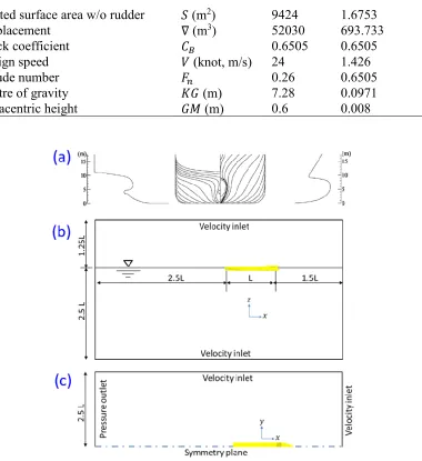
Table 1 shows the principal particulars of the KCS. In this study, the CFD simulation was modelled using the scale factor of 75, as used for the towing test [15]. Fig. 5 depicts an overview of the body plan, side profiles of the KCS, as well as the boundary conditions and the dimensions of the computational domain. The velocity inlet and pressure outlet boundary conditions were applied as the inlet and outlet boundary conditions. For the representation of deep water and infinite air conditions, the boundary conditions of the side walls, bottom and top of the domain were set to the velocity inlet. The vertical centre plane was defined as the symmetry plane. It is of note that the model ship was free to sink and trim in the simulations. Table 1 Principal particulars of the KCS in full-scale and model-scale, adapted from Kim et al. [26] and Larsson et al. [27]

Parameters Full-scale Model-scale

Scale factor 𝜆 1 75

Length between the perpendiculars 𝐿_𝑃𝑃 (m) 230 3.0667

Length of waterline 𝐿_𝑊𝐿 (m) 232.5 3.1

Beam at waterline 𝐵_𝑊𝐿 (m) 32.2 0.4293

Depth 𝐷 (m) 19.0 0.2533

Wetted surface area w/o rudder 𝑆 (m2_{) 9424 1.6753}

Displacement ∇ (m3_{) 52030 693.733}

Block coefficient 𝐶𝐵 0.6505 0.6505

Design speed 𝑉 (knot, m/s) 24 1.426

Froude number 𝐹_𝑛 0.26 0.6505

Centre of gravity 𝐾𝐺 (m) 7.28 0.0971

Metacentric height 𝐺𝑀 (m) 0.6 0.008

Fig. 5 Computational domain and boundary conditions of the KCS model ship simulation, (a) body plane and side profiles of the KCS, adapted from Kim et al. [26], (b) profile view, (c) top view

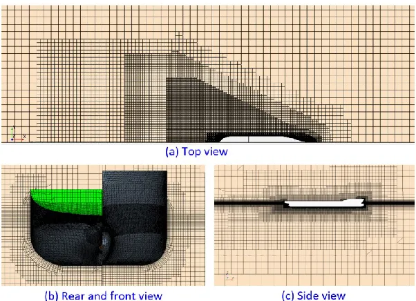
2.3. Mesh generation

Mesh generation was performed using the built-in automated meshing tool of STAR-CCM+. Trimmed hexahedral meshes were used. Local refinements were made for finer grids in the critical regions, such as the regions near the free surface, leading and trailing edges of the flat plate, the bulbous bow of the KCS hull. The prism layer meshes were generated for near-wall refinement. The first layer cell thicknesses on the surfaces of the plate and the model ship were chosen such that the 𝑦+ _{values are}

always higher than 30, and also higher than the roughness Reynolds number values, 𝑘+_{, as suggested by}

Fig. 6 Volume mesh of the flat plate simulation

Fig. 7 Volume mesh of the KCS model ship simulation

3. Result

3.1. Verification

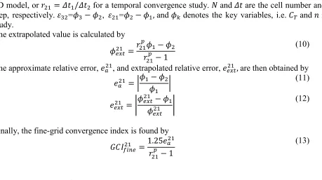
spatial convergence studies, it can also be used for a temporal convergence study, as similarly used by Tezdogan et al. [29] and Terziev et al. [30].

According to Celik et al. [31] the apparent order of the method, 𝑝𝑎, is determined by

𝑝_𝑎 = 1

ln(𝑟₂₁)| ln | 𝜀₃₂

𝜀₂₁| + 𝑞(𝑝𝑎) |

(7)

𝑞(𝑝𝑎) = ln (

𝑟₂₁𝑝𝑎_{− 𝑠} 𝑟₃₂𝑝𝑎_{− 𝑠})

(8)

𝑠 = 𝑠𝑖𝑔𝑛 (𝜀32 𝜀21

) (9)

where, 𝑟21 and 𝑟32 are refinement factors given by 𝑟21= √𝑁3 1/𝑁2 for a spatial convergence study of a

3D model, or 𝑟21= 𝛥𝑡1/𝛥𝑡2 for a temporal convergence study. 𝑁 and 𝛥𝑡 are the cell number and time

step, respectively. 𝜀32=𝜙3 − 𝜙2, 𝜀21=𝜙2− 𝜙1, and 𝜙𝑘 denotes the key variables, i.e. 𝐶𝑇 and 𝑛 in this

study.

The extrapolated value is calculated by

𝜙_𝑒𝑥𝑡21 = 𝑟21

𝑝

𝜙₁− 𝜙₂ 𝑟₂₁𝑝 − 1

(10)

The approximate relative error, 𝑒_𝑎21_{, and extrapolated relative error, 𝑒}

𝑒𝑥𝑡21, are then obtained by

𝑒𝑎21= |

𝜙₁− 𝜙₂ 𝜙1

| (11)

𝑒𝑒𝑥𝑡21 = |

𝜙_𝑒𝑥𝑡21 − 𝜙1

𝜙_𝑒𝑥𝑡21 |

(12)

Finally, the fine-grid convergence index is found by

𝐺𝐶𝐼_{𝑓𝑖𝑛𝑒}21 =1.25𝑒𝑎

21

𝑟₂₁𝑝 − 1

(13)

3.1.1. Spatial convergence study

For the spatial convergence study, three different meshes were generated based on different resolutions, which are referred to as fine, medium and coarse meshes corresponding the cell numbers of 𝑁₁, 𝑁₂, and 𝑁₃. Table 2 depicts the required parameters for the calculation of the spatial discretisation error. The simulations were conducted in the smooth surface condition, with the inlet speeds of 4.5 m/s (𝑅𝑒_𝐿 = 5.6 × 106) and 1.426 m/s (𝐹𝑛 = 0.26, 𝑅𝑒𝐿 = 3.7 × 106), for the flat plate and the KCS model

simulations respectively. The total resistance coefficients, 𝐶𝑇, were used as the key variables.

As indicated in the table, the numerical uncertainties of the fine meshes (𝐺𝐶𝐼_{𝑓𝑖𝑛𝑒}21 _{) for the flat plate and}

KCS hull simulations are 0.79% and 0.10% respectively. For accurate predictions, the fine meshes were used for further simulations in this study.

Table 2 Parameters used for the discretisation error for the spatial convergence study, key variable: 𝐶_𝑇

𝑁₁ 451,271 601,355

𝑁₂ 913,737 887,428

𝑁₃ 2,258,814 1,306,433

𝑟21 1.57 1.21

𝑟32 1.42 1.21

𝜙1 3.710E-03 4.471E-03

𝜙2 3.753E-03 4.461E-03

𝜙₃ 3.836E-03 4.494E-03

𝜀₃₂ 8.34E-05 3.23E-05

𝜀₂₁ 4.30E-05 -9.08E-06

𝑠 1 -1

𝑒𝑎21 1.16% 0.20%

𝑞 3.82E-01 -6.14E-03

𝑝a 2.31E+00 6.53E+00

𝜙_𝑒𝑥𝑡21 _{3.686E-03 4.474E-03}

𝑒𝑒𝑥𝑡21 0.63% -0.08%

𝐺𝐶𝐼_{𝑓𝑖𝑛𝑒}21 0.79% 0.10%

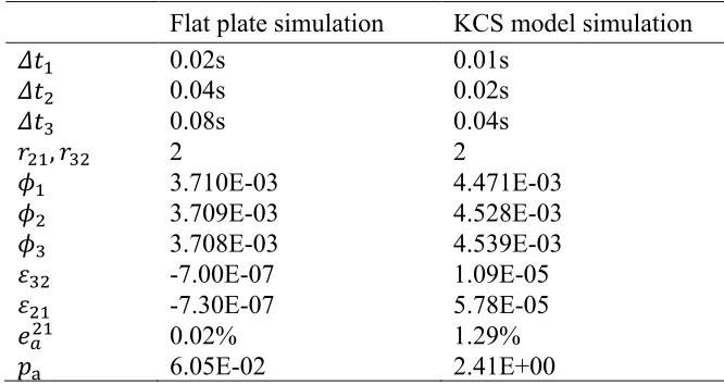
3.1.2. Temporal convergence study

For the temporal convergence study, three different time steps, namely 𝛥𝑡1, 𝛥𝑡2, and 𝛥𝑡3, were used for

the simulations using the fine meshes. Table 3 shows the required parameters for the calculation of the temporal discretisation error. The simulations were conducted in the smooth surface condition, with the inlet speeds of 4.5 m/s (𝑅𝑒_𝐿 = 5.6 × 106_{) and 1.426 m/s (𝐹𝑛 = 0.26, 𝑅𝑒}

𝐿 = 3.7 × 106), for the flat

plate and KCS model simulations respectively. The total resistance coefficients, 𝐶𝑇, were used as the key

variables.

As indicated in the table, the numerical uncertainties (𝐺𝐶𝐼_𝛥𝑡21_{1) of the flat plate and the KCS hull}

simulations are 0.57% and 0.27% respectively when the smallest time steps are used (𝛥𝑡1). For accurate

predictions, the smallest time steps (𝛥𝑡1) were used for further simulations in this study.

Table 3 Parameters used for the discretisation error for the temporal convergence study, key variable: 𝐶_𝑇

Flat plate simulation KCS model simulation

𝛥𝑡1 0.02s 0.01s

𝛥𝑡2 0.04s 0.02s

𝛥𝑡3 0.08s 0.04s

𝑟21, 𝑟32 2 2

𝜙₁ 3.710E-03 4.471E-03

𝜙₂ 3.709E-03 4.528E-03

𝜙₃ 3.708E-03 4.539E-03

𝜀₃₂ -7.00E-07 1.09E-05

𝜀₂₁ -7.30E-07 5.78E-05

𝑒𝑎21 0.02% 1.29%

𝜙𝑒𝑥𝑡21 3.727E-03 4.457E-03

𝑒_𝑒𝑥𝑡21 -0.46% 0.30%

𝐺𝐶𝐼_𝛥𝑡21₁ 0.57% 0.37%

3.2. Validation

3.2.1. Flat plate simulation

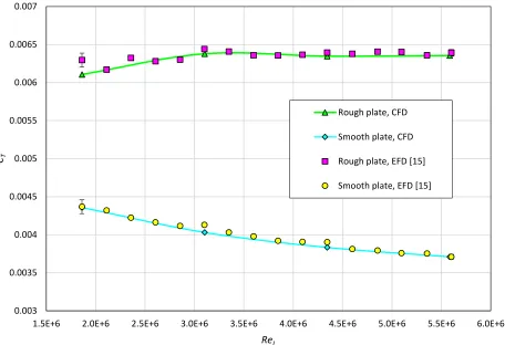
Fig. 8 compares the total resistance coefficient, 𝐶_𝑇, values in the smooth and rough surface conditions predicted from the current CFD simulations and the experimental data of Song et al. [15]. The CFD simulations were conducted at the speed range of 1.5 − 4.5 m/s with 1.0 m/s interval, with the corresponding Reynolds numbers of 𝑅𝑒𝐿 = 1.9 − 5.6 × 106.

As shown in the figure, the 𝐶_𝑇 values of the smooth flat plate predicted from the CFD simulations show an excellent agreement with the experimental data. Similarly, a good agreement was achieved between the CFD and EFD results for the 𝐶_𝑇 of the rough flat plate apart from the under-prediction of the 𝐶_𝑇 value at the lowest speed (1.5 m/s, 𝑅𝑒_𝐿 = 1.9 × 106_{). Considering the uncertainty of the experimental}

𝐶𝑇 values and the roughness function (Fig. 3) as well as the numerical uncertainty of the simulation, this

slight under-prediction is believed to be acceptable.

Fig. 8 Total resistance coefficient, 𝐶_𝑇, of the towed flat plate in the smooth and rough surface

conditions, predicted from the current CFD simulations and the experimental data of Song et al. [15]

3.2.2. KCS model ship simulation

Although the use of the modified wall-function approach is validated against the flat plate towing tests, this does not necessarily guarantee the validity of using this method to predict the roughness effect on the ship resistance of a 3D hull. Therefore, this section presents the comparison between the CFD approach and the experimental result of the towing test of the KCS model ship in the smooth and rough surface conditions [15].

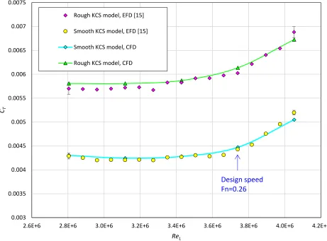
Fig. 9 shows a comparison of the 𝐶𝑇 values of the KCS model ship predicted from the current CFD

simulations and the experimental results [15]. The CFD simulations were conducted at the speed range of 1.07 − 1.54 m/s, which correspond to the full-scale speed range 18 − 26 knots with 2 knots interval. The corresponding Reynolds numbers are 𝑅𝑒𝐿 = 2.8 − 4.1 × 106, while the Froude numbers are 𝐹𝑛 =

0.195 − 0.282. In both the smooth and rough surface conditions, the 𝐶𝑇 values predicted from the CFD

simulations agrees well with the experimental 𝐶_𝑇 values. Therefore, it suggests that the modified wall-function approach can accurately predict the effect of hull roughness on the total ship resistance, which includes the 3D effects.

It is of note that this is the first validation of the CFD modelling of hull roughness against ship model test.

0.003 0.0035 0.004 0.0045 0.005 0.0055 0.006 0.0065 0.007

1.5E+6 2.0E+6 2.5E+6 3.0E+6 3.5E+6 4.0E+6 4.5E+6 5.0E+6 5.5E+6 6.0E+6

CT

Re_L

Rough plate, CFD

Smooth plate, CFD

Rough plate, EFD [15]

Fig. 9 Total resistance coefficient, 𝐶_𝑇, of the KCS model ship in the smooth and rough surface conditions, predicted from the current CFD simulations and the experimental data [15]

3.3. Effect of hull roughness on the ship resistance components

In the previous section, the validity of the modified wall-function approach was demonstrated for predicting the effect of hull roughness on the ship total resistance. Therefore, it is worth to utilise the benefits of using CFD for better understanding the roughness effect on the individual ship resistance components. Decompositions of the ship total resistance into the different resistance components are presented in this section.

Before investigating the effect of hull roughness on the resistance components, it would be timely to re-state these components in detail. The resistance coefficients can be obtained by dividing the drag, 𝑅, with the dynamic pressure, 1

2𝜌𝑉

2_{, and the wetted surface area of the ship hull, 𝑆, as}

𝐶 = 𝑅

1 2 𝜌𝑆𝑉2

(14) 0.003

0.0035 0.004 0.0045 0.005 0.0055 0.006 0.0065 0.007 0.0075

2.6E+6 2.8E+6 3.0E+6 3.2E+6 3.4E+6 3.6E+6 3.8E+6 4.0E+6 4.2E+6

CT

ReL

Rough KCS model, EFD [15]

Smooth KCS model, EFD [15]

Smooth KCS model, CFD

Rough KCS model, CFD

The total ship resistance coefficient, 𝐶_𝑇, can be decomposed into the two main components; the frictional resistance coefficient, 𝐶𝐹, and the residuary resistance coefficient, 𝐶𝑅, given by

𝐶_𝑇 = 𝐶_𝐹+ 𝐶_𝑅 (15)

The residuary resistance is can be further divided into the viscous pressure resistance coefficient, 𝐶_𝑉𝑃, and the wave making resistance coefficient, 𝐶𝑊, given by

𝐶_𝑅 = 𝐶_𝑉𝑃+ 𝐶_𝑊 (16)

𝐶𝑇 = 𝐶𝐹+ 𝐶𝑉𝑃+ 𝐶𝑊 (17)

The viscous pressure or also known as form drag is broadly assumed to be proportional to the frictional resistance [32], with the use of form factor, 𝑘, as given

𝐶_𝑉𝑃 = 𝑘𝐶_𝐹 (18)

𝐶_𝑇 = 𝐶_𝐹+ 𝑘𝐶_𝐹 + 𝐶_𝑊 (19)

𝐶𝑇 = (1 + 𝑘)𝐶𝐹+ 𝐶𝑊 (20)

The sum of frictional resistance and the viscous pressure resistance is also referred to as viscous resistance, 𝐶_𝑉, as

𝐶_𝑉 = 𝐶_𝐹 + 𝐶_𝑉𝑃= (1 + 𝑘)𝐶_𝐹 (21)

3.3.1. Frictional resistance and residuary resistance

The total resistance coefficients, 𝐶𝑇, were divided into the frictional resistance coefficient, 𝐶𝐹, and the

residuary resistance coefficient, 𝐶_𝑅, by simply decomposing the total drag acting on the ship into the shear and pressure force components.

The 𝐶_𝐹 and 𝐶_𝑅 values of the KCS model in the smooth and the rough conditions are shown in Fig. 10. The 𝐶_𝐹 values for the rough KCS model remain rather consistent with the Reynolds numbers, while the smooth 𝐶𝐹 values show a decreasing trend. This can be explained by the fact that 𝐶𝐹 tends to lose its

dependency to the Reynolds number when it approaches the fully rough regime [33], as similarly observed by other studies [15-16, 20].

On the other hand, the rough case shows larger 𝐶𝑅 values than the smooth case, but the differences

become smaller as the Reynolds number increases (which can be more clearly seen in Fig. 11). To fine the rationale behind this observation, further investigation was carried out by decomposing the 𝐶𝑅 into

Fig. 10 𝐶𝐹 and 𝐶𝑅 values of the KCS model in the smooth and rough surface conditions

3.3.2. Viscous pressure and wave making resistance

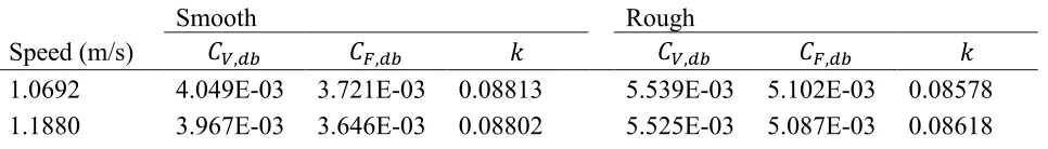
In order to decompose the 𝐶_𝑅 into the 𝐶_𝑉𝑃 and 𝐶_𝑊, as similar approach was used as Song et al. [20]. To obtain the form factor values, double-body flow simulations were conducted by modifying the CFD model. In the double-body simulations, the free surface is replaced by a symmetry plane such that no wave can be generated and hence only the viscous resistance (𝐶_𝑉 = 𝐶_𝐹+ 𝐶_𝑉𝑃) exists [34, 35]. Then the form factor values, 𝑘, were calculated as

𝑘 =𝐶𝑉,𝑑𝑏 𝐶𝐹,𝑑𝑏

− 1 (22)

where 𝐶_{𝑉,𝑑𝑏} and 𝐶_{𝐹,𝑑𝑏} denote the viscous resistance and frictional resistance obtained from the double-body flow simulations. Table 4 shows the form factor values for the smooth and rough KCS models for the given speeds. As observed by Song et al [20] the form factor values showed decreases due to the hull roughness.

Table 4 𝐶_𝑉, 𝐶_𝑉𝑃 and 𝑘 values obtained from the double-body simulations

Smooth _Rough

Speed (m/s) 𝐶𝑉,𝑑𝑏 𝐶𝐹,𝑑𝑏 𝑘 𝐶𝑉,𝑑𝑏 𝐶𝐹,𝑑𝑏 𝑘

1.0692 4.049E-03 3.721E-03 0.08813 5.539E-03 5.102E-03 0.08578 1.1880 3.967E-03 3.646E-03 0.08802 5.525E-03 5.087E-03 0.08618

0 0.001 0.002 0.003 0.004 0.005 0.006

2.6E+6 2.8E+6 3.0E+6 3.2E+6 3.4E+6 3.6E+6 3.8E+6 4.0E+6 4.2E+6

CF

and

CR

ReL

CF smooth

CF rough

CR smooth

CR rough

1.3068 3.899E-03 3.583E-03 0.08792 5.477E-03 5.041E-03 0.08652 1.4255 3.839E-03 3.529E-03 0.08783 5.513E-03 5.077E-03 0.08597 1.5443 3.787E-03 3.482E-03 0.08776 5.532E-03 5.095E-03 0.08582

Using the form factor values, 𝑘, 𝐶𝑉𝑃 and 𝐶𝑊 were calculated as

𝐶_𝑉𝑃= 𝑘𝐶_𝐹 (23)

𝐶𝑊 = 𝐶𝑅− 𝐶𝑉𝑃 (24)

Fig. 11 compares the 𝐶_𝑅, 𝐶_𝑉𝑃 and 𝐶_𝑊 values of the KCS model in the smooth and rough surface conditions. As similarly observed by Song et el. [20], the rough KCS model has larger 𝐶_𝑉𝑃 values than the smooth KCS model, but the contributions of 𝐶_𝑉𝑃 values in 𝐶_𝑅 show decreasing trends with increasing speeds (thus, the Reynolds number). On the other hand, the wave making resistance, 𝐶_𝑊, values for both the smooth and rough cases increase with the speed. The discrepancy between smooth and rough 𝐶_𝑊 is small at low speeds, but smooth 𝐶_𝑊 becomes larger than rough 𝐶_𝑊 as the speed increases.

Subsequently, the differences between the smooth and rough 𝐶_𝑅 become smaller at higher Reynolds numbers as the roughness effects on the 𝐶_𝑉𝑃 and 𝐶_𝑅 cancel each other. This observation of the increased 𝐶𝑉𝑃 and decreased 𝐶𝑊 values agrees with the findings of Song et al. [20].

Fig. 11 𝐶𝑅, 𝐶𝑉𝑃 and 𝐶𝑊 values of the KCS model in the smooth and rough surface conditions

0.0000 0.0003 0.0006 0.0009 0.0012 0.0015

2.6E+6 2.8E+6 3.0E+6 3.2E+6 3.4E+6 3.6E+6 3.8E+6 4.0E+6 4.2E+6

CR ,CVP

and

CW

Re_L

CR smooth

CR rough

CVP smooth

CVP rough

CW smooth

CW rough

3.4. Effect of hull roughness on the flow characteristics

This section compares the flow characteristics around the KCS model in the smooth and rough surface conditions at its design speed (𝑉_{𝑚𝑜𝑑𝑒𝑙} = 1.43 m/s, 𝐹𝑛 = 0.26, 𝑅𝑒_𝐿 = 3.7 × 106_).

3.4.1. Velocity field

Fig. 12 and 13 compare the mean axial velocity contours around the stern of the KCS model ship in both the surface conditions. The mean axial velocity was normalised by dividing the velocity with the advance speed of the ship. As shown in the figures, the hull roughness resulted in the decelerated flow around the stern and it enlarged the wake field. This enlarged wake region can be closely related to the distribution of the surface pressure at the stern (16), which leads to the increase in the viscous pressure resistance.

Another notable feature is the increased boundary layer thickness due to the hull roughness as shown in Fig. 12. It can be more clearly seen in Fig. 14, where the boundary layer is represented by the slices of axial velocity contours limited to 𝑉_𝑥/𝑉_{𝑚𝑜𝑑𝑒𝑙} = 0.9. This increased boundary layer thickness results in increased momentum loss and hence the frictional resistance, as shown in Fig. 10. This roughness effect on the boundary layer thickness leads to increased momentum loss and thus leads to increased skin friction. This observation is in correspondence with the experimental and numerical studies of other researchers [16, 20, 36, 37].

As the enlarged wake field due to the hull roughness was observed in Fig. 13, the nominal wake fractions of the smooth and rough KCS model were calculated. Fig. 15 illustrates the distribution of the local wake fraction, 𝑤_𝑛′ _{= 1 − 𝑉}

𝑥/𝑉𝑚𝑜𝑑𝑒𝑙, at the propeller plane (𝑥 = 0.0175𝐿𝑝𝑝). The inner and outer circles

denote the hub diameter and the propeller diameter, respectively. From the figure, it is evident that the hull roughness increases the local wake fraction significantly, and it led to a 35% increase in the mean nominal wake fraction 𝑤_𝑛 (0.31 to 0.42).

Fig. 13 Mean axial velocity contours at 𝑥 = 0.0175𝐿_𝑝𝑝

Fig. 15 Local wake fraction, 𝑤_𝑛′, at the propeller plane

3.4.2. Pressure field

Fig. 16 illustrates the distribution of the dynamic pressure along the hull in the smooth and rough surface conditions. The dynamic pressure was normalised by dividing them with the dynamic pressure, 1

2𝜌𝑉 2_{. It}

can be seen from the figure that the rough case has a smaller pressure at the stern (i.e. reduced pressure recovery). This smaller surface pressure at the stern due to the hull roughness can be related to the increased viscous pressure resistance, 𝐶𝑉𝑃, in Fig. 11.

3.4.3. Wave profile

Fig. 17 compares the wave patterns around the KCS model in the smooth and rough surface conditions. It is seen from the figure that the wave elevations around the hull are reduced by the hull roughness. This roughness effect on the wave pattern can be also seen in Fig. 18, which compares the wave elevation along the line with constant 𝑦 = 0.1509𝐿_𝑝𝑝. This roughness effect on the wave profile is in accordance with the reduced 𝐶_𝑊 values due to the hull roughness as shown in Fig. 11. This observation also agrees with the findings of Demirel et al. [16] and Song et al. [20].

Fig. 17 Wave pattern around the KCS model

Fig. 18 Wave elevation along a line with constant 𝑦 = 0.1509𝐿𝑝𝑝

4. Concluding remarks

In this study, the CFD approach to predict the effect of hull roughness on the ship resistance was validated against the experiment of a towed flat plate and a model ship in the smooth and rough surface conditions. In order to simulate the effect of the surface roughness, a roughness function model was proposed based on the roughness function of Song et al. [15] and employed in the wall-function of the CFD model.

-0.005 -0.003 -0.001 0.001 0.003

-1.5 -1 -0.5 0 0.5 1 1.5

z/L

pp

x/Lpp

Spatial and temporal convergence studies were performed using the Grid convergence Index (GCI) method, to estimate the numerical uncertainties of the proposed CFD models and to determine sufficient grid-spacings and time steps.

Fully nonlinear unsteady RANS simulations of the flat plate and the KCS model ship were conducted in the smooth and rough surface conditions. The simulation results showed excellent agreements with the experimental data of Song et al. [15] in both the smooth and rough surface conditions. This result suggests that the CFD approach (i.e. modified wall-function approach) can accurately predict not only the roughness effect on the skin friction, but also the total resistance of a 3D hull.

The total ship resistance predicted from the CFD simulations in the smooth and rough conditions were decomposed into individual resistance components. Significant increases in the frictional resistance, 𝐶_𝐹, due to the hull roughness were found. Increases in the viscous pressure resistance, 𝐶𝑉𝑃, and decreases in

the wave making resistance, 𝐶𝑊, were also observed due to the hull roughness.

The effect of hull roughness on the flow characteristics around the hull was also examined. By comparing the velocity filed around the KCS model in the smooth and rough conditions, a decelerated flow and enlarged wake field were observed downstream of the stern, as well as the increased boundary layer thickness. It was found that the hull roughness reduces the pressure recovery at the stern, which leads to increased viscous pressure resistance. Smaller wave elevation due to the hull roughness was also noted, which is closely related to the smaller wave making resistance for the rough case.

This study has provided the first experimental validation of the CFD approach to predict the effect of hull roughness on the ship total resistance by comparing the simulations with the model ship towing test. Apart from the effect of hull roughness, there have been several studies predicting the effect of roughness on the blades on the propeller performances using the same CFD approach. However, this approach has not been experimentally validated for propellers. Therefore, future pieces of work may include a validation study of the CFD simulations to predict the roughness effect on propellers.

5. Acknowledgements

It should be noted that the results were obtained using the ARCHIE-WeSt High Performance Computer (www.archie-west.ac.uk) based at the University of Strathclyde.

6. References

1. Tezdogan, T., & Demirel, Y. K. (2014). An overview of marine corrosion protection with afocus on cathodic protection and coatings. Brodogradnja, 65, 49–59.

2. Demirel, Y. K., Uzun, D., Zhang, Y., Fang, H.-C., Day, A. H., & Turan, O. (2017). Effect of barnacle fouling on ship resistance and powering. Biofouling, 33(10), 819-834.

doi:10.1080/08927014.2017.1373279

3. Townsin, R. L. (2003). The Ship Hull Fouling Penalty. Biofouling, 19(sup1), 9-15. doi:10.1080/0892701031000088535

4. Granville, P. S. (1958). The frictional resistance and turbulent boundary layer of rough surfaces. J. Ship Res., 2(3), 52-74.

5. Granville, P. S. (1978). Similarity-law characterization methods for arbitrary hydrodynamic roughnesses. Retrieved from Bethesda, MD:

7. Schultz, M. P. (2004). Frictional Resistance of Antifouling Coating Systems. Journal of Fluids Engineering, 126(6), 1039-1047. doi:10.1115/1.1845552

8. Shapiro, T. A. (2004). The Effect of Surface Roughness on Hydrodynamic Drag and Turbulence. Retrieved from

9. Schultz, M. P., & Flack, K. A. (2007). The rough-wall turbulent boundary layer from the hydraulically smooth to the fully rough regime. Journal of Fluid Mechanics, 580, 381-405. doi:10.1017/S0022112007005502

10.Flack, K. A., & Schultz, M. P. (2010). Review of Hydraulic Roughness Scales in the Fully Rough Regime. Journal of Fluids Engineering, 132(4), 041203-041203-041210. doi:10.1115/1.4001492 11.Schultz, M. P., Bendick, J. A., Holm, E. R., & Hertel, W. M. (2011). Economic impact of

biofouling on a naval surface ship. Biofouling, 27(1), 87-98. doi:10.1080/08927014.2010.542809 12.Demirel, Y. K. (2015). Modelling the Roughness Effects of Marine Coatings and Biofouling on

Ship Frictional Resistance. (PhD), University of Strathclyde, Glasgow.

13.Li, C., Atlar, M., Haroutunian, M., Norman, R., & Anderson, C. (2019). An investigation into the effects of marine biofilm on the roughness and drag characteristics of surfaces coated with different sized cuprous oxide (Cu2O) particles. Biofouling, 1-19. doi:10.1080/08927014.2018.1559305 14.Demirel, Y. K., Song, S., Turan, O., & Incecik, A. (2019). Practical added resistance diagrams to

predict fouling impact on ship performance. Ocean Engineering, 186, 106112. doi:https://doi.org/10.1016/j.oceaneng.2019.106112

15.Song, S., Dai, S., Demirel, Y. K., Atlar, M., Day, S., & Turan, O. (2019 in progress). Experimental and theoretical study of the effect of hull roughness on ship resistance. Journal of Ship Research. 16.Demirel, Y. K., Turan, O., & Incecik, A. (2017). Predicting the effect of biofouling on ship

resistance using CFD. Applied Ocean Research, 62, 100-118. doi:https://doi.org/10.1016/j.apor.2016.12.003

17.Atlar, M., Yeginbayeva, I. A., Turkmen, S., Demirel, Y. K., Carchen, A., Marino, A., & Williams,

D. (2018). A Rational Approach to Predicting the Effect of Fouling Control Systems on “In

-Service” Ship Performance. GMO SHIPMAR, 24(213), 5-36.

18.Demirel, Y. K., Khorasanchi, M., Turan, O., Incecik, A., & Schultz, M. P. (2014). A CFD model for the frictional resistance prediction of antifouling coatings. Ocean Engineering, 89, 21-31. doi:https://doi.org/10.1016/j.oceaneng.2014.07.017

19.Farkas, A., Degiuli, N., & Martić, I. (2018). Towards the prediction of the effect of biofilm on the

ship resistance using CFD. Ocean Engineering, 167, 169-186. doi:https://doi.org/10.1016/j.oceaneng.2018.08.055

20.Song, S., Demirel, Y. K., & Atlar, M. (2019b). An investigation into the effect of biofouling on the ship hydrodynamic characteristics using CFD. Ocean Engineering, 175, 122-137.

doi:https://doi.org/10.1016/j.oceaneng.2019.01.056

21.Owen, D., Demirel, Y. K., Oguz, E., Tezdogan, T., & Incecik, A. (2018). Investigating the effect of biofouling on propeller characteristics using CFD. Ocean Engineering.

doi:https://doi.org/10.1016/j.oceaneng.2018.01.087

22.Song, S., Demirel, Y. K., & Atlar, M. (2019a). An investigation into the effect of biofouling on full-scale propeller performance using CFD. Paper presented at the 38th International Conference on Ocean, Offshore & Arctic Engineering, Glasgow.

23.Song, S., Demirel, Y. K., & Atlar, M. (2019 in progress). Effect of biofouling on ship self-propulsion performance. Applied Ocean Research

25.Menter, F. R. (1994). Two-Equation Eddy-Viscosity Turbulence Models for Engineering Applications. AIAA Journal, 32(8), 1598-1605.

26.Kim, W. J., Van, S. H., & Kim, D. H. (2001). Measurement of flows around modern commercial ship models. Experiments in Fluids, 31(5), 567-578. doi:10.1007/s003480100332

27.Larsson, L., Stern, F., & Visonneau, M. (2013). CFD in Ship Hydrodynamics—Results of the Gothenburg 2010 Workshop. In L. Eça, E. Oñate, J. García-Espinosa, T. Kvamsdal, & P. Bergan (Eds.), MARINE 2011, IV International Conference on Computational Methods in Marine Engineering: Selected Papers (pp. 237-259). Dordrecht: Springer Netherlands.

28.Richardson, L. F. (1910). The approximate arithmetical solution by finite differences of physical problems involving differential equations, with an application to the stresses in a masonry dam. Transcations of the Royal Society of London. Series A, 210, 307-357.

29.Tezdogan, T., Demirel, Y. K., Kellett, P., Khorasanchi, M., Incecik, A., & Turan, O. (2015). Full-scale unsteady RANS CFD simulations of ship behaviour and performance in head seas due to slow steaming. Ocean Engineering, 97, 186-206. doi:https://doi.org/10.1016/j.oceaneng.2015.01.011 30.Terziev, M., Tezdogan, T., Oguz, E., Gourlay, T., Demirel, Y. K., & Incecik, A. (2018). Numerical

investigation of the behaviour and performance of ships advancing through restricted shallow waters. Journal of Fluids and Structures, 76, 185-215.

doi:https://doi.org/10.1016/j.jfluidstructs.2017.10.003

31.Celik, I. B., Ghia, U., Roache, P. J., Freitas, C. J., Coleman, H., & Raad, P. E. (2008). Procedure for Estimation and Reporting of Uncertainty Due to Discretization in CFD Applications. Journal of Fluids Engineering, 130(7), 078001-078001-078004. doi:10.1115/1.2960953

32.Lewis, E. V. (1988). Principles of Naval Architecture : Resistance, Propulsion and Vibration: 2 Jersey City: The Society of Naval Architects and Marine Engineers.

33.Nikuradse, J. (1933). Laws of flow in rough pipes. NACA Technical Memorandum, 1292.

34.Raven, H. C., Ploeg, A. v. d., Starke, A. R., & Eça, L. (2008). Towards a CFD-based prediction of ship performance - progress in predicting full-scale resistance and scale effects. Paper presented at the RINA MArine CFD Conference, London.

35.Van, S.-H., Ahn, H., Lee, Y.-Y., Kim, C., Hwang, S., Kim, J., . . . Park, I.-R. (2011). Resistance characteristics and form factor evaluation for geosim models of KVLCC2 and KCS. Paper

presented at the The 2nd International Conference on Advanced Model Measurement Technology for the EU Maritime Industry, Newcastle upon Tyne, UK.

36.Schultz, M. P., & Flack, K. A. (2005). Outer layer similarity in fully rough turbulent boundary layers. Experiments in Fluids, 38(3), 328-340. doi:10.1007/s00348-004-0903-2