Numerical simulations of a shock interacting with multiple magnetized clouds

magnetized clouds

.

White Rose Research Online URL for this paper:

http://eprints.whiterose.ac.uk/82593/

Version: Published Version

Article:

Aluzas, R, Pittard, JM, Falle, SAEG et al. (1 more author) (2014) Numerical simulations of

a shock interacting with multiple magnetized clouds. Monthly Notices of the Royal

Astronomical Society, 444 (1). 971 - 993. ISSN 0035-8711

https://doi.org/10.1093/mnras/stu1501

[email protected]

https://eprints.whiterose.ac.uk/

Reuse

Unless indicated otherwise, fulltext items are protected by copyright with all rights reserved. The copyright

exception in section 29 of the Copyright, Designs and Patents Act 1988 allows the making of a single copy

solely for the purpose of non-commercial research or private study within the limits of fair dealing. The

publisher or other rights-holder may allow further reproduction and re-use of this version - refer to the White

Rose Research Online record for this item. Where records identify the publisher as the copyright holder,

users can verify any specific terms of use on the publisher’s website.

Takedown

If you consider content in White Rose Research Online to be in breach of UK law, please notify us by

Numerical simulations of a shock interacting with multiple magnetized

clouds

R. Al¯uzas,

J. M. Pittard,

S. A. E. G. Falle

and T. W. Hartquist

2_{Department of Applied Mathematics, University of Leeds, Woodhouse Lane, Leeds LS2 9JT, UK}

Accepted 2014 July 23. Received 2014 July 23; in original form 2014 April 29

A B S T R A C T

We present 2D adiabatic magnetohydrodynamic simulations of a shock interacting with groups of two or three cylindrical clouds. We study how the presence of a nearby cloud influences the dynamics of this interaction, and explore the resulting differences and similarities in the evolution of each cloud. The understanding gained from this small-scale study will help to interpret the behaviour of systems with many 10s or 100s of clouds. We observe a wide variety of behaviour in the interactions studied, which is dependent on the initial positions of the clouds and the orientation and strength of the magnetic field. We find (i) some clouds are stretched along their field lines, whereas others are confined by their field lines; (ii) upstream clouds may accelerate past downstream clouds (though magnetic tension can prevent this); (iii) clouds may also change their relative positions transverse to the direction of shock propagation as they ‘slingshot’ past each other; (iv) downstream clouds may be offered some protection from the oncoming flow as a result of being in the lee of an upstream cloud; (v) the cycle of cloud compression and re-expansion is generally weaker when there are nearby neighbouring clouds; (vi) the plasmaβin cloud material can vary rapidly as clouds collide with one another, but low values ofβare always transitory. This work is relevant to studies of multiphase regions, where fast, low-density gas interacts with dense clouds, such as in circumstellar bubbles, supernova remnants, superbubbles and galactic winds.

Key words: hydrodynamics – shock waves – turbulence – ISM: clouds – ISM: kinematics and dynamics – ISM: supernova remnants.

1 I N T R O D U C T I O N

The interstellar medium (ISM) is recognized to be highly dynamic. At any given time a substantial quantity of gas is found to be transit-ing between several different phases of thermal equilibrium. Such transitions are driven by a variety of heating and cooling mecha-nisms. Heating is dominated by vigorous energy input from high-mass stars, including their intense ionizing radiation fields, their powerful winds and their terminal supernova explosions. Heating also occurs via the conversion of gravitational potential energy and from the impact of extragalactic material. Cooling is achieved via a multitude of radiative processes and through adiabatic expansion.

Given these conditions, it is not uncommon for hot, high-speed material to interact with cooler, dense material (often referred to as clouds). Knowledge of the dynamical and thermal behaviour of gas in such interactions is necessary for a complete understanding of the nature of the ISM. For instance, in starburst galaxies, the energy input from high-mass stars inflates superbubbles which can

⋆_{E-mail:[email protected]}

burst out of their host. However, the properties of such flows may be controlled by their interaction with small clouds which dominate the mass in such regions. These clouds may be destroyed and their mass incorporated into the hot phase, a process known as ‘mass loading’. This behaviour is a key ingredient in models of galaxy formation and evolution (e.g. Sales et al.2010), but is currently not calculated self-consistently in them. On the other hand, the compression of clouds by the flow may ultimately trigger new star formation.

By far the best studied case is that of a shock hitting an isolated spherical cloud. The hydrodynamics of the interaction have been re-ported in a number of papers in which the cloud density contrast,χ, and the shock Mach number,M, have been varied (e.g. Stone & Norman 1992; Klein, McKee & Colella 1994; Nakamura et al.

2006). The effect of other processes in this interaction has also been studied, such as magnetic fields (e.g. Mac Low et al.1994; Shin, Stone & Snyder2008), radiative cooling (e.g. Mellema, Kurk & R¨ottgering2002; Fragile et al.2004; Yirak, Frank & Cunningham

2010) and thermal conduction (e.g. Orlando et al.2005,2008). The turbulent nature of the destruction of clouds has been investigated too (e.g. Pittard et al.2009; Pittard, Hartquist & Falle2010). In the purely hydrodynamic case clouds are destroyed via the growth

2014 The Authors

at University of Leeds on January 22, 2015

http://mnras.oxfordjournals.org/

of Kelvin–Helmholtz (KH) and Rayleigh–Taylor (RT) instabilities. The interaction becomes milder at lower shock Mach numbers, with the most marked differences occurring when the post-shock gas is subsonic with respect to the cloud. Cloud density contrastsχ 103_{are required for material stripped off the cloud to form a long}

‘tail-like’ feature. Efficient cooling causes the cloud to fragment. The presence of magnetic fields can strongly affect the inter-action. In 2D axisymmetry, magnetic fields parallel to the shock normal suppress Richtmyer–Meshkov (RM) and KH instabilities, and reduce mixing. The magnetic field is amplified behind the cloud due to shock focusing and forms a ‘flux rope’ (Mac Low et al.1994). In contrast, in 3D simulations with strong fields perpendicular or oblique to the shock normal the shocked cloud becomes sheet-like at late times, and oriented parallel to the post-shock field. The cloud then fragments into vertical or near-vertical columns (Shin et al.

2008). More recent work including magnetic fields, anisotropic thermal conduction and radiative cooling of 3D shock–cloud inter-actions finds that intermediate-strength fields are most effective at producing long-lasting density fragments – stronger fields prevent compression while weak fields do not sufficiently insulate the cloud to allow efficient cooling (e.g. Johansson & Ziegler2013).

Relatively few investigations of the interaction of a flow with multiple clouds exist. The response of a clumpy and magnetized medium to a source of high pressure was considered by Elmegreen (1988), who derived jump conditions for cloud collision fronts un-der a continuum approximation. This work was extended using a multifluid formalism by Williams & Dyson (2002), who showed that shocks can rapidly broaden and thus create a more benign en-vironment which aids the survival of multiphase structure passing through the shock.

Simulations in which the interaction of a flow over numerous obstacles is studied in detail are only just becoming feasible. How-ever, it is clear that the flow responds differently to the presence of a group of clouds, with a global bowshock forming when the clouds are relatively close (e.g. Poludnenko, Frank & Blackman2002; Pit-tard et al.2005; Al¯uzas et al.2012, hereafterPaper I). The degree to which the nature of the flow changes depends on the relative amount of mass added to the flow by destruction of the clouds, i.e. the mass-loading factor. Simulations extending Poludnenko’s work to higher mass-loading factors were presented byPaper I. This work found that the global flow is not strongly affected by the presence of clouds with density contrasts ofχ₌102_{, as it evolves similarly to a}

region of equivalent, uniform density. However, significant changes arise when the cloud density contrast increases toχ₌103_{. In this}

case the total mass in the clouds becomes dominant at a much lower volume fraction (equivalently a lower total cross-section of the clouds). The resulting interaction does not affect the structure of the shock much, but significantly mass loads the post-shock flow. This ongoing mass loading of the flow as the clouds are destroyed can cause the shock to decelerate even after it has left the clumpy region.

The evolution of a cloud also changes when additional clouds are nearby. In isolation, clouds lose most of their mass through KH instabilities, with the largest scale instabilities taking some time to grow. In mass-loaded flows, instabilities develop more easily due to the turbulent nature of the flow. Clouds are also ablated more quickly due to the higher density of the mass-loaded post-shock flow.

Fig.19inPaper Ishows that the cloud lifetimes can be reduced by as much as 40 per cent, compared to the single-cloud lifetime at the same resolution. However, we have since discovered a prob-lem with our previous analysis which for computational reasons

was conducted on low-resolution single- and multicloud runs. The problem is that the development of KH instabilities is significantly slowed at lower resolution and clouds instead lose mass through direct ablation. The latter is a stronger effect in the multicloud sim-ulations due to the higher density of the flow caused by material mixing into it from clouds further upstream. Thus our previous low-resolution simulations inPaper Iwere biased against the devel-opment of KH instabilities but not against direct ablation, leading us to erroneously conclude that clouds in multicloud runs have shorter lifetimes. We now find from a high-resolution comparison of the lifetime of clouds in single- and multicloud simulations that the clouds are destroyed in essentially the same time.1

Magnetohydrodynamic (MHD) studies of the interaction of a shock with a single cloud show that the field is amplified not so much in the shear layers and vortices but rather in regions of compression: ahead of the cloud for perpendicular shocks where field lines bunch up, and in a ‘flux rope’ behind the cloud where the flow converges for the parallel-shock case (Mac Low et al.1994). These simulations show that magnetic fields limit mixing and fragmentation, but do not stop it completely, and provide support to the cloud perpendicular to the field lines. Our goal in this paper is to determine the degree to which neighbouring clouds change this picture. In particular, we are interested in the amplification of the magnetic field and the presence of magnetically dominated regions withβ <1. Can clouds present in regions of enhanced magnetic field enhance the field further or does it saturate? Because of the complex nature of the interaction and the many free parameters which now also include the positions and separations of clouds, we limit this current study to interactions involving two or three clouds. For computational reasons we also limit our study to 2D (i.e. our clouds are infinite cylinders). This work will serve as a basis for future work exploring the interaction of a shock with many 10s and 100s of clouds in 2D and 3D.

The outline of this paper is as follows. In Section 2 we intro-duce our numerical method. Section 3 details the results of our simulations. In Section 4 we summarize and conclude.

2 M E T H O D

The computations were performed using adaptive mesh refinement (AMR) code,mg. The ideal MHD equations are solved using a linear Riemann solver for most cases and an exact solver when there is a large difference between the two states (Falle, Komis-sarov & Joarder1998). Piecewise linear cell interpolation is used. The scheme is second-order accurate in space and time, and is

1_{However, the nature of the destruction is a little different. In multicloud}

simulations, clouds initially lose mass a little more slowly than in single-cloud simulations because of the reduction in the shock speed brought about by the mass loading of the flow. However, as the shocked cloud moves further downstream it encounters increasing post-shock density relative to the single-cloud case, and this increases the rate of ablation slightly. The net effect is that the overall lifetime of the cloud is very similar to the single-cloud case. Having said this, single-clouds with a higher density contrast than the

majority of neighbouring cloudsdoseem to still be destroyed more quickly

than their single-cloud counterparts. We tentatively suggest this is because of the dense shell of ablated material which overruns them and increases their rate of mass loss from ablation [all similar clouds are destroyed by

one cloud destruction length (1LCD) behind the shock front, and so are not

affected by the shell, whereas the denser clouds still exist at the time they are overrun by the shell]. This effect will be investigated in a forthcoming paper.

at University of Leeds on January 22, 2015

http://mnras.oxfordjournals.org/

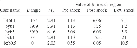
single- and multicloud simulations performed. The value of the plasmaβ

in the pre-shock (i.e.β0) and post-shock regions is also provided, as well

as its approximate value in the bowshock region.

Value ofβin each region

Case name Bangle Ma Pre-shock Post-shock Bow-shock

b15b1 15◦ _{2.91 1.13 6.06 7.1}

byb1 89◦._{9 2.91 1.13 1.25 1.2}

byb5 89◦._{9 6.16 5.06 6.05 5.5}

bxb1 0◦ _{2.91 1.13 12.4 21}

bxb0.5 0◦ 2.03 0.55 6.05 10.5

supplemented by a divergence cleaning technique described in Ded-ner et al. (2002).

The simulations were performed on 2DXYCartesian grids, so that the clouds are actually infinite cylinders. Two grids (G0_andG1₎

cover the entire domain. Finer grids are added where they were needed and removed where they are not. Refinement and derefine-ment are controlled by differences in the solutions on the coarser grids with a tolerance of 1 per cent in the conserved quantities spec-ified. Each refinement level increased the resolution in all directions by a factor of 2. The time step on gridGn_ist

0/2n, wheret0

was the time step onG0_{. Refinement is performed on a cell-by-cell}

basis rather than patches.

A typical grid extendedX_∈[₋50:190]rclandY ∈[−50:50]rcl,

whererclis the cloud radius (identical clouds are assumed). Inflow

boundary conditions were used at the negativeXboundary, being set by the shock jump conditions. Free inflow/outflow conditions were used at the other three boundaries. Simulations were performed with two sets of resolutions: 32 cells per cloud radius (R32) and 128 cells

per cloud radius (R128). The lower resolution runs used seven grid

levels, withx₌2rclon theG0grid, while the higher resolution

simulations used eight grid levels, withx₌1rclon theG0grid.

The simulations set up two or three clouds with a cloud density contrast ofχ₌100 and with soft edges following the density profile as specified in Pittard et al. (2009) withp1=10. In all simulations

the sonic Mach number of the shock was 3. The strength of the magnetic field and its orientation to the shock was varied. Values for the Alfv´enic Mach number, the pre-shock field angle and the plasma β in different regions are given in Table 1. A different advected scalar is used for each cloud to track the cloud material. The time is measured in units of the cloud crushing time-scale,tcc=

χ1/2_r

cl/vb, wherevbis the shock velocity in the ambient medium.

The bowshock reaches theYboundaries at around 7.5tcc and the

simulations are terminated shortly afterwards. Adiabatic behaviour is assumed withγ₌5/3.

3 R E S U LT S

The collective interactions between a large number of clouds can be incredibly complex. To better understand them we begin by review-ing the basic behaviour of a shock strikreview-ing an isolated, magnetized, cylindrical cloud. We then investigate the simplest of multiple cloud cases, that of two clouds, before applying the insight from the two-cloud simulations to simulations with three two-clouds. Single-two-cloud simulations are named using the formatsc bAbB, where the ‘sc’ in-dicates that it is of a single cloud, the ‘A’ indicates the orientation of the field (‘x’, ‘15’ and ‘y’ indicate parallel, oblique and perpendic-ular shocks) and ‘B’ indicates the value of the pre-shock plasmaβ. Two-cloud simulations are named using the formats2wYoX bAbB

(or often using the shortened formswYoXorwYoX bAbB). Similarly,

Figure 1. The morphology of interactions of a shock with a single cylin-drical cloud. The calculations are in 2D, the sonic Mach number is 3 and

the Alfv´enic Mach number is 2.91 (β0=1.13). The shock is (a) parallel,

(b) oblique and (c) perpendicular. The cloud is initially positioned at the ori-gin The grey-scale shows the logarithmic density and magnetic field lines

are also shown. The contour indicates regions with low plasmaβand low

momentum (β <1 andρ|u|<0.5×ρ_ps|u_ps|). The time of the interaction

ist=4tcc.

three-cloud simulations are named using the formats3wRaθbAbB

(again also with shortened versions).wYoXandwRaθ identify the relative positions of clouds, see Sections 3.2 and 3.3, respectively for further details.

3.1 Single-cloud interactions

3.1.1 Parallel shocks

We begin by reviewing the morphology of the 2D interaction of a shock with a single magnetized, cylindrical cloud. In the parallel field case a ‘flux rope’ forms directly behind the cloud: the flow converging behind the cloud compresses the field lines, thus in-creasing the magnetic pressure which prevents the post-shock flow from entering it (see Fig.1a). As a result the ‘flux rope’ not only has a low plasmaβ, but it also has very low momentum. These two conditions (β <1 andρ_|u|<0.5×ρ_ps|u_ps|) specify the ‘flux rope’ region in the parallel field case, but can also be met in other field arrangements.

Another important feature in the flow are the ‘wings’. This is a region or regions alongside the flux rope which delineates where the flow is stripping material away from the cloud. This region shows up

at University of Leeds on January 22, 2015

http://mnras.oxfordjournals.org/

in the magnetic field structure of simulations with parallel shocks as the reversal of the magnetic field. In general the ‘wings’ are shielded from the momentum of the flow, although occasionally they may contain higher density fragments stripped off the upstream cloud.

3.1.2 Oblique shocks

In our oblique shock simulations a pre-shock field orientation of

θ0=15◦was chosen to be a representative oblique field case. This

givesθps=45◦in the post-shock medium. When an oblique shock

interacts with an isolated cylindrical cloud we find that the field lines wrap around the cloud keeping its cross-section roughly circular in shape (see Fig. 1b). Field lines above the cloud become nearly parallel to the direction of shock propagation2_{and some material is}

stripped off along them. Field lines below the cloud span a range of angles, with the region immediately upstream of the cloud having field lines nearly parallel to the shock front. Field amplification and ‘shielding’ (i.e. where gas has minimal exposure to the ambient flow – e.g. gas in the lee of a cloud) now occur in distinct, but overlapping regions. The cloud is accelerated downstream and also laterally (in Fig. 1b) the cloud is seen to move to lower Y. The asymmetry of the cloud’s motion reflects the asymmetric bunching and tensioning of the field lines and the direction of the post-shock flow. Note that because the cloud in this simulation is actually an infinite cylinder field lines cannot easily slip past it. If the cloud were spherical we would expect some splitting and rearranging of the field, which could significantly change the forces acting on the cloud.

3.1.3 Perpendicular shocks

In the perpendicular field case, the magnetic field is initially ampli-fied directly upstream of the cloud where the flow stagnates against it (see Fig.1c). Because field lines cannot slip around the surface of the cloud (again due to its nature as an infinite cylinder), mag-netic pressure and field tension continue to build with the result that the cloud accelerates rapidly downstream (compare the positions of the clouds in Fig.1). This rapid acceleration acts to reduce the magnetic pressure and tension. Again we expect the evolution to be quite different to that of a spherical cloud.

3.2 Two-cloud interactions

We now investigate the interaction of magnetized shocks with two closely positioned clouds. We first examine the morphology of the interaction, and then discuss the acceleration of the clouds and the evolution of the plasma β. The two-cloud arrangements are specified by their ‘width’, which is the lateral distance between the cloud centres in units of the cloud radius (i.e. the separation of the clouds in the ‘y’ direction), and by their ‘offset’, which is the longitudinal distance between the clouds (i.e. their separation in the ‘x’ direction).t₌0 is defined as the time that the shock reaches the leading edge of the more upstream of the two clouds.

3.2.1 Parallel shocks

In interactions with a parallel shock, the presence of a second cloud alongside the first cloud has the effect of suppressing the lateral

2_{The post-shock flow is about}

−7◦_{to the shock normal.}

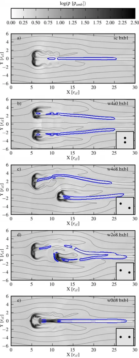
re-expansion of the cloud. This is easily seen when comparing the single-cloud simulationscand the two-cloud simulationw4o0(in panels a and b of Fig.2, respectively). The flow between the clouds is slowed and squeezed, but accelerates once past the clouds. The initial high pressure between the clouds drops due to the Bernoulli effect, causing the initial outwardly directed orientation of the flux ropes to change towards an inwardly directed orientation.3

As the initial position of one of the clouds is moved downstream the lateral suppression of the upstream cloud is reduced and it evolves more like the single cloud case. However, the downstream cloud is still much more affected by lateral confinement (see the results forw4o8shown in Fig.2c).

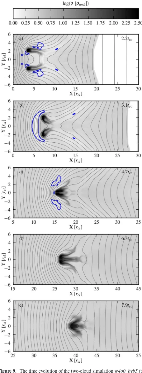
The morphology of the downstream cloud is dependent on the ‘width’ as well as the ‘offset’, though the ‘width’ is the dominant parameter. The simulationsw4o8,w2o8andw0o8shown in panels (c)–(e) of Fig.2illustrate the diversity of the downstream cloud morphology, which we find can be categorized into three main types. When there is a sufficient gap between the clouds for the flow to weave through (e.g. as in simulationw4o8– see Fig.2c), the downstream cloud is confined in a similar manner as if there was a cloud alongside it. In contrast, when a cloud is directly behind an upstream cloud (e.g. as in simulationw0o8 – see Fig.2e), it falls in its ‘flux rope’. The cloud is shielded from the flow and does not accelerate. The flow that tries to converge behind the upstream cloud (which forms the ‘flux rope’) instead now converges on the downstream cloud, compressing it into an elongated shape. The upstream cloud is also affected by the presence of the downstream cloud. As it accelerates towards the downstream cloud the tenuous gas between them is compressed, modifying the morphology of the upstream cloud in advance of their collision.

The third type of behaviour occurs when the downstream cloud is positioned such that it lies in the ‘wings’ of the flow around the upstream cloud (e.g. see simulationw2o8– shown in panel d of Fig.2). To better understand the nature of this interaction we also show the time evolution of this simulation in Fig.3. We find that the ‘flux ropes’ of the two clouds merge downstream, while the magnetic field near the clouds becomes highly irregular. The latter is affected by the fact that the background flow becomes quite turbulent as it tries to force its way between the clouds at the same time as the clouds are distorted and influenced by the flow. The turbulent nature of the flow appears to be quite efficient at stripping material away from the downstream cloud. In spite of this, the cloud is mostly confined into anrcl-sized clump and does

not spread very far along its field lines. Similar behaviour for the downstream cloud is also seen in simulationw4o8at late times as the upstream cloud expands and the downstream cloud is pushed into the shielded region.

3.2.2 Oblique shocks

We now study the interaction of an oblique shock with two cylindri-cal clouds. As the oblique magnetic field is not symmetric about the

x-axis it provides another direction to supplement the ‘upstream’ and the ‘downstream’ designations. We define the ‘upfield’ cloud as the one whose field lines encounter the shock front first. In the cases considered the upfield cloud is almost always the ‘top’ cloud (i.e. has an initial positive ‘y’ position). The exceptions are simulations

w2o-8where the two clouds lie on roughly the same field lines, and

3_{This behaviour is also seen in purely hydrodynamic simulations (Pittard}

et al.2005).

at University of Leeds on January 22, 2015

http://mnras.oxfordjournals.org/

Figure 2. Snapshots of the morphology of (a) an individual cloud and (b)–

(e) two clouds with varying separation and offset att=4tcc. In all cases the

magnetic field is parallel to the shock normal andβ0=1.13. The contour

again shows the ‘flux rope’ (β <1 andρ|u|<0.5×ρ_ps|u_ps|), while the

grey-scale shows the logarithmic density. The two-cloud simulations are identified by the initial ‘width’ and ‘offset’ of the clouds – the relative

positions of the cloud att=0 are shown in the inset of each panel (shown

at reduced scale). The resolution isR32. At higher resolution the fine scale

structure changes somewhat, but the general features of the flow and their dependence on the initial arrangement of the clouds remain unchanged.

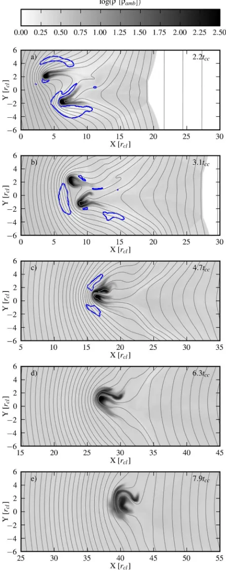
Figure 3. The time evolution of the two-cloud simulations2w2o8(the

clouds are positioned with an initial ‘width’=2rcl and ‘offset’=8rcl).

The magnetic field is parallel to the shock normal andβ0 =1.13. The

logarithmic density and magnetic field evolution are shown at timest=2.2,

3.1, 4.7, 6.3 and 7.9tcc(top to bottom). The contour shows the ‘flux rope’

(β <1 andρ|u|<0.5×ρ|u|_ps). In this simulation the downstream cloud is confined by the presence of the upstream cloud. Note the changes in the

x- andy-coordinates in each panel.

at University of Leeds on January 22, 2015

http://mnras.oxfordjournals.org/

w2o-12which was chosen specifically to have the ‘bottom’ cloud as the ‘upfield’ one.

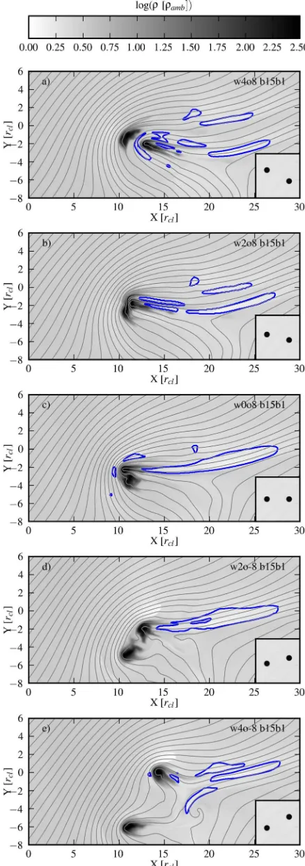
Figs4and5compare snapshots of the density and magnetic field structure of a single cloud case and a range of two-cloud arrange-ments att₌ 4tcc. Note that a negative ‘offset’ signifies that the ‘top’ cloud is the downstream one. In all cases the field geome-try causes the clouds to accelerate downwards (to more negative

ypositions) at the same time that they are accelerated downstream (to more positive xpositions). We see that the nature of the in-teraction is significantly modified by the presence of the second cloud, and that it depends on the relative initial positions of the clouds. In some cases the downstream cloud is protected from the oncoming flow by its position in the lee of the upstream cloud (e.g. as seen in simulationw4o4in Fig.4, and in simulationsw4o8

and w2o8 in Fig.5). In other cases the downstream cloud feels the full fury of the oncoming flow (e.g. as seen for the top cloud in simulation w4o-4in Fig. 4and simulation w4o-8in Fig.5). Whether the top or bottom cloud accelerates fastest downstream depends on their relative orientation to the shock and the field (e.g. in simulationw4o4in Fig.4and in simulationsw4o8andw2o8in Fig.5the top cloud accelerates fastest downstream, while in sim-ulationsw4o-4andw2o-12in Fig.4and simulationsw2o-8and

w4o-8in Fig.5the bottom cloud does so). Note that the bottom cloud in simulationw0o8shown in Fig.5is initially the upstream cloud.

Because the field lines are now forced to bend around two clouds, in many cases the region where the magnetic field is parallel to the direction of the shock propagation becomes larger and another region where the field is perpendicular extends between the two clouds (see e.g. simulationsw4o4,w4o0andw4o-4in Fig.4). The clouds are also a lot less circular than compared to the case of a single cloud with an oblique field (compare any panel in Figs4and

5with panel a in Fig.4). Stripping now frequently occurs along multiple directions.

In many cases the wrapping of the field lines causes the top cloud to accelerated downwards (i.e. to more negativeypositions) faster than the bottom cloud is accelerated in this direction. This can cause the clouds to either collide or come as close together as allowed by the magnetic pressure which builds between them (see simulations

w4o8andw2o8in Fig.5). In other cases we find that the upstream cloud can become the most downstream cloud as the interaction evolves. Fig.6shows a time sequence from simulationw2o-8b15b1

which shows how the upstream cloud (in this case the bottom cloud) overtakes the downstream (top) cloud. Once the bottom cloud moves into the ‘lee’ of the top cloud it experiences reduced confinement forces and begins to diffuse. Simultaneously the top cloud becomes more exposed to the oncoming flow and experiences another episode of compression. This type of behaviour is seen in a large range of oblique simulations.

3.2.3 Perpendicular shocks

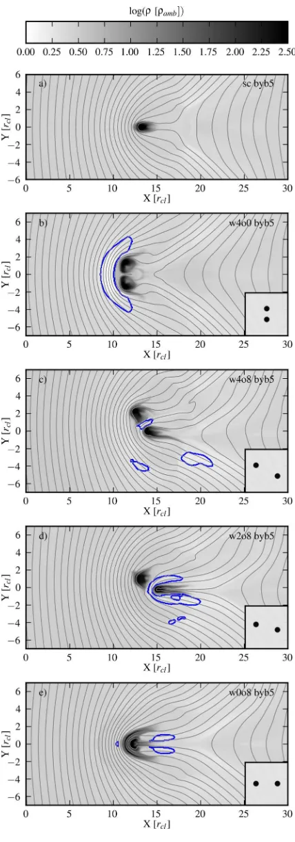
Finally, we study the interaction of a perpendicular shock with two cylindrical clouds. Figs7and8compare snapshots of the density and magnetic field structure of interactions of a single cloud and two clouds with a perpendicular shock at t₌ 4tcc. In Fig.7the

plasmaβof the pre-shock medium isβ0=5.06, whereas the field

is significantly stronger in Fig.8(β0=1.13). As the field strength

increases the magnetic field increasingly controls the dynamics of the interaction. This is evident from the suppressed instabilities and cloud mixing, enhanced diffusion of the cloud along the field lines,

Figure 4. Snapshots att=4tccof the morphology and field structure of

shock–cloud simulations with an oblique magnetic field (θ0 =15◦ and

β0 =1.13). The top panel shows the interaction with a single cylindrical

cloud (sc b15b1), while the remaining panels show the interaction with two

cylindrical clouds. The grey-scale shows the logarithmic density while the contour shows the ‘flux rope’.

at University of Leeds on January 22, 2015

http://mnras.oxfordjournals.org/

Figure 5. Two-cloud oblique-field snapshots like those in Fig.4but for a

fixed cloud ‘offset’ of 8rcland varied ‘width’.

Figure 6. The evolution of the two-cloud simulations2w2o-8(the clouds

are positioned with an initial ‘width’=2rcl and ‘offset’=−8rcl). The

magnetic field is oblique to the shock normal (θ =15◦ andβ0=1.13).

The logarithmic density and magnetic field evolution are shown at times

t₌2.2, 3.1, 4.7, 6.3 and 7.9tcc(top to bottom). The contour shows the ‘flux

rope’ (β <1 andρ|u|<0.5×ρ|u|_ps). In this simulation the cloud which

is initially upstream (i.e. the bottom cloud) is accelerated past the top cloud

such that it becomes the most downstream cloud fort4.7tcc.

at University of Leeds on January 22, 2015

http://mnras.oxfordjournals.org/

Figure 7. As Fig.4but with perpendicular magnetic fields andβ0=5.06.

The time of each snapshot is againt=4tcc.

Figure 8. As Fig.7but withβ0 =1.13. The time of each snapshot is

againt=4tcc. The stronger magnetic field now controls the dynamics more

compared to the simulations shown in Fig.7.

at University of Leeds on January 22, 2015

http://mnras.oxfordjournals.org/

greater acceleration of the clouds downstream and straighter field lines in Fig.8versus Fig.7.

We again find that the presence of a second cloud has a major influence on the nature of the interaction. As the field lines wrap around the two clouds they are driven towards each other very rapidly. If clouds lie on the same field line they merge into a sin-gle clump (see the time evolution of simulationsw4o0in Figs9

and10). During this process a large continuous region of high mag-netic pressure forms upstream of the clouds. Comparison of Figs9

and10 reveals that there is some numerical diffusion present in theR32simulations but that the same general behaviour occurs.4If

the clouds do not lie on the same field line, then a build up in the magnetic pressure between the clouds prevents their merger (see simulationw4o8in Fig.7where the contour between the clouds highlights the region of high magnetic pressure). Lazarian (2013) argues that the actual reconnection diffusion in turbulent plasmas might be quite fast and there might be a resemblance between nu-merical diffusion and magnetic reconnection in turbulent flows.

If the clouds are aligned or nearly aligned with the direction of shock propagation the downstream cloud is shielded from the oncoming flow by the upstream cloud which moves very close towards it (see simulationsw2o8andw0o8in Fig.7). In such cases, the magnetic field lines between the clouds prevent the clouds from merging. The downstream cloud is compressed laterally by the upstream cloud which wraps around it.

In some cases, clouds which are initially separated quite widely can be driven towards each other to end up in a very compact arrangement. This behaviour is shown in Fig.11, which shows the evolution of the interaction in simulationw4o4. In such cases, shock compression of the field lines naturally reduces the ‘offset’ between the clouds, while their ‘width’ is easily reduced by their motion along the field lines. In this example the downstream cloud moves towards the low-pressure region behind the upstream cloud and away from the high (magnetic) pressure region around the outside edge of the combined clouds. The field lines between the clouds prevent complete merging in this instance.

3.2.4 Cloud velocities

In simulations with a parallel or perpendicular magnetic field the clouds generally develop a smally component to their velocity which often draws the clouds towards each other (see e.g. simulation

w2o8in Fig.3and simulationw4o4_byb5in Fig.11).

However, the velocity evolution of a cloud is generally far more significant when the magnetic field is oblique. A clear and system-atic distinction between thexvelocity component of the ‘top’ and ‘bottom’ clouds can be seen in Fig.12. The ‘upstream’ cloud ac-celerates first which is the ‘top’ cloud for positive ‘offset’ and the ‘bottom’ cloud if the ‘offset’ is negative. Initially, thexvelocity in the ‘bottom’ cloud grows at a rate similar to the isolated cloud case (compare the dotted lines for simulationsw4o-8,w4o4andw4o0

with the black crosses). Thevxvelocity of each of these clouds

over-shoots slightly the post-shock flow value, as does the isolated cloud.

4_{Because of this difference in numerical diffusion we find that the}

de-gree to which clouds merge when they do not lie on the same field lines is dependent on the resolution, with higher resolution simulations better able to prevent mixing and maintain distinct clouds in such cases (stronger

fields also tend to keep clouds separate).R128 resolution is also

neces-sary for accurate calculation of the plasmaβin some circumstances – see

Section 3.2.5.

Figure 9. The time evolution of the two-cloud simulationw4o0_byb5(the

clouds are positioned with an initial ‘width’=4rcland ‘offset’=0rcl)

The magnetic field is perpendicular to the shock normal (β0=5.06). The

logarithmic density and magnetic field evolution are shown at times 2.2, 3.1,

4.7, 6.3 and 7.9tcc(top to bottom). The contour shows the ‘flux rope’ (β <1

andρ|u|<0.5×ρ|u|_ps). See also the second panel in Fig.7.

at University of Leeds on January 22, 2015

http://mnras.oxfordjournals.org/

Figure 10. As Fig.9but with a resolution of 128 cells per cloud radius (instead of 32).

Figure 11. The time evolution of the two-cloud simulationw4o4_byb5(the

clouds are positioned with an initial ‘width’=4rcl and ‘offset’=4rcl).

The magnetic field is perpendicular to the shock normal (β0=5.06). The

logarithmic density and magnetic field evolution are shown at timest=2.2,

3.1, 4.7, 6.3 and 7.9tcc(top to bottom). The contour shows the ‘flux rope’

(β <1 andρ|u|<0.5×ρ|u|_ps). In this simulation the clouds accelerate towards each other with the upstream cloud eventually wrapping around the downstream cloud.

at University of Leeds on January 22, 2015

http://mnras.oxfordjournals.org/

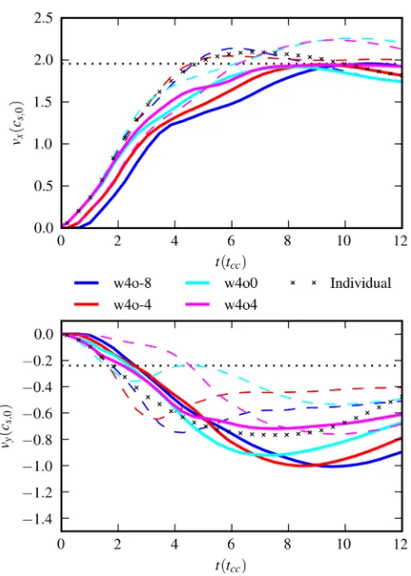
Figure 12. Evolution of thex(top panel) andy(bottom panel) cloud velocity components in simulations with two clouds and oblique magnetic fields. The velocity is normalized by the sound speed of the intercloud ambient medium. The initial ‘width’ of the cloud distribution is identical in each simulation

(being 4rcl), while the ‘offset’ is varied. In each panel the ‘top’ cloud in

the distribution is shown using solid lines while dashed lines correspond to the ‘bottom’ cloud. The dotted black line shows the intercloud velocity of the post-shock flow. Also shown is the velocity evolution of a single-cloud simulation (indicated by the black crosses).

In contrast, the acceleration of the ‘top’ cloud is notably slower after about 2.5tccand in all simulations it reaches the post-shock flow

value without any overshoot.

The bottom panel of Fig.12shows the evolution of theyvelocity component of the clouds. In the single cloud case the cloud sig-nificantly overshoots the velocity of the post-shock flow which has a normalized valuevy≈ −0.25cs, 0. The single cloud reaches its

peakyvelocity of_≈−0.8cs, 0att≈7.5tcc, before decelerating. At

late times we would expect the cloudvyto asymptote towards that

of the post-shock flow but this clearly takes place on time-scales in excess of 12tcc. Theyvelocity component of the clouds in the

two-cloud simulations follows the same broad behaviour of initial acceleration, overshoot of the equilibrium value and deceleration towards the post-shock speed, but there are significant differences in the details. The ‘top’ cloud accelerates downward slowly initially, but significantly overshoots the isolated cloud case later on (unless the ‘top’ cloud is also the ‘upstream’ one (e.g.w4o4), in which case its behaviour is closer to the isolated cloud). In contrast the ‘bottom’ cloud initially accelerates faster than the isolated cloud, but starts slowing down much sooner (reaching a peak velocity of ≈−0.65cs, 0att≈3tccforw4o-4). Simulationw4o4is again the

exception – as the ‘downstream’, ‘bottom’ cloud is shielded from the flow it accelerates very slowly initially. Finally, we note that

Figure 13. The evolution of thexandyseparations of the clouds in two-cloud simulations with oblique magnetic fields. A sign change (i.e. move-ment across the horizontal black line) represents a switch in relative position.

some clouds (e.g. the ‘bottom’ cloud in simulationw4o0) undergo a second period of acceleration.

Overall, we find that the ‘bottom’ cloud moves faster in the ‘x’ direction and the ‘top’ cloud moves faster in the ‘y’ direction. Thus if initially the ‘upstream’ cloud is the ‘bottom’ one then the upstream cloud will overtake the downstream cloud. This is high-lighted in the top panel of Fig.13where we see that the clouds swap relative positions (i.e. cross the horizontal black line) in simulations

w4o-8,w4o-4,w4o-2andw4o-1. It is also observed in simulation

w2o-8as shown in Fig.6.

However, we also find that the ‘top’ and ‘bottom’ clouds swap their relativeypositions in all of the simulations with ‘width’₌4rcl

that we have investigated. This is shown in the lower panel of Fig.13

where all the simulations cross the horizontal black line, irrespective of the initial ‘offset’. We observe that a swap-over even occurs in simulations like w4o-8, where the ‘bottom’ cloud is the first to accelerate and the separation between the clouds actually grows until 6tcc (in this case the swap-over occurs att>10tcc). Fig.6

shows the swap-over process occurring in simulationw2o-8att_≈

8tcc(here the ‘bottom’ cloud moves underneath and then behind

the ‘top’ cloud).

3.2.5 The plasmaβ

Of the simulations performed, the parallel shock simulations with

β0=1.13 (i.e. modelsbxb1) have the highest post-shockβ(∼12,

see Table1). It is in these simulations that instabilities are least suppressed by the magnetic field. Simulations with single clouds reveal that the results are sensitive to resolution, with a convergence

at University of Leeds on January 22, 2015

http://mnras.oxfordjournals.org/

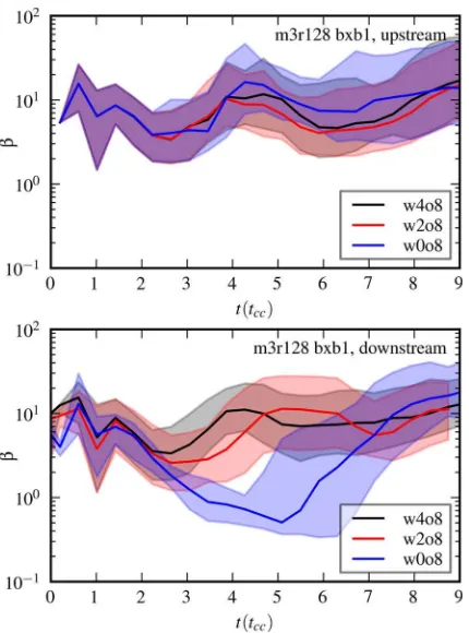
Figure 14. The time evolution of theβdistributions for upstream (top panel)

and downstream (bottom panel) clouds inR128two-cloud simulations with

parallel magnetic fields and pre-shockβ0=1.13. The initial cloud ‘offset’

is 8 while the initial cloud ‘width’ is varied. The solid line shows the median

βvalue and the area between the 25th and 75th percentiles is shaded.

study indicating that of order 100 cells per cloud radius are needed for accurate results (in keeping with previous work of adiabatic hydrodynamical shock–cloud interactions – see e.g. Klein et al.

1994; Pittard et al.2009). In contrast, the presence of additional clouds disturbs the flow such that longer wavelength instabilities play a more important role. This reduces the resolution requirements in multicloud simulations. However, in order to compare like-with-like, we perform the following analysis ofβin the parallel shock simulations using resolution R128 for the multicloud simulations

too.

We first study how the distribution ofβin the simulations with a parallel shock changes as the initial positions of the clouds are varied. In each of the following figures we show the time evolution of the distribution of the plasmaβof the cloud material (the dis-tribution is calculated over all cells in the simulation upstream of the shock front but is weighted by the amount of cloud material in each cell).βchanges with time as the cloud is first compressed, and then re-expands. At late timesβshould approach the value in the post-shock flow. This behaviour can be seen in Fig.14.

We find that varying the initial cloud ‘offset’ has no real effect on theβdistributions when the initial cloud ‘width’ is greater than the diameter of the clouds. In Fig.14we show how the evolution of

βdepends instead on the initial ‘width’ of the cloud distribution for simulations withβ0=1.13. We find that the upstream cloud is not

affected in thew2o8simulation, but the growth ofβis delayed by 1tccin the downstream cloud (compare the red and blue lines in the

bottom panel of Fig.14between 3t/tcc5). Note, though that

this delay is not seen in thebxb0.5case where the magnetic field is more dominant.

Figure 15. Evolution of the harmonic average ofβin material from the ‘top’ cloud (top panel) and the ‘bottom’ cloud (bottom panel) in two-cloud

simulations with an oblique magnetic field (whereβ0=1.13 andθ0=15◦).

The initial cloud positions have a ‘width’ of 4rcland varying ‘offset’. The

evolution ofβin isolated clouds is also shown [for simulations with 32 (R32)

and 128 (R128) cells per cloud radius].

In thew0o8case (see Fig.2e), the downstream cloud falls inside the flux rope andβdrops to_∼0.5 in the downstream cloud until the clouds collide. Theβdistribution of the upstream cloud is also affected in this case – β is generally slightly higher due to the increased pressure downstream. The same behaviour is seen if the magnetic field is made slightly stronger. For example, in simulations withβ0=0.55 (modelsbxb0.5) the minimumβis still around 0.5

in the downstream cloud, while the increase of the plasmaβin the upstream cloud is even more prominent.

We find that simulations with an oblique magnetic field are much less sensitive to resolution, and we are able to use simulations with a resolution of 32 cells per cloud radius. We adopt the harmonic mean as the average for theβ statistics in these simulations: it demonstrates good convergence because it is not influenced by a small number of cells with highβwhere the flow is poorly resolved. The harmonic mean is thus a good estimator for the ‘typical’βvalue of cloud material, and it generally falls in between the 30th and 50th percentile values.

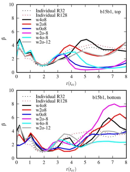
Figs15and16show the evolution of the harmonic mean ofβin material from the ‘top’ and ‘bottom’ clouds of various simulations. The ‘top’ cloud is the upstream one if the ‘offset’ is positive, and is the ‘upfield’ cloud in all simulations exceptw2o-12andw2o-8. These figures also show the variation ofβin simulations with a single individual cloud. In Fig.15 we see the effect of varying the ‘offset’ value of the initial cloud distribution while keeping the initial distribution ‘width’ fixed at a value of 4rcl. In contrast, in

Fig.16the initial distribution ‘width’ is varied while the ‘offset’ is kept at 8 or 12rcl.

at University of Leeds on January 22, 2015

http://mnras.oxfordjournals.org/

Figure 16. As Fig.15but for clouds in simulations with an initial ‘offset’

of 8rcland varying ‘width’. The upstream cloud is identified as the ‘top’

cloud in simulationw0o8.

These figures reveal thatβis significantly reduced in the ‘top’ cloud when it is the upstream one (see modelsw4o2andw4o4in Fig.15, and modelsw4o8,w2o8andw0o8in Fig.16). In model

w2o8we see that β <1 during the period 4t/tcc 7; Fig. 5

shows that the clouds collide at this time. In fact, the collision of the clouds is responsible for the lowβvalues in the material of the top cloud in all of these simulations, and also in simulationw0o8

(where lowβvalues occur in the upstream cloud). In contrast, we find thatβin material in the ‘bottom’ cloud is similar to that in the isolated cloud or slightly higher.

When the ‘top’ cloud is the ‘downstream’ one, the harmonic mean ofβin both of the clouds evolves similarly to the evolution ofβin an isolated cloud. Exceptions to this behaviour occur only for the bottom cloud in simulationsw4o-2andw4o0(see Fig.15) and simu-lationw2o-8(see Fig.16); in these cases the ‘bottom’ cloud reaches much higherβvalues. The reason for this difference is evident from Fig.6, which reveals that in simulationw2o-8the ‘bottom’ cloud overtakes the ‘top’ cloud and becomes the ‘downstream’ cloud at the time whenβstarts growing. The same behaviour also occurs in the other two cases. For example, in simulationw4o0the bottom cloud crosses a line perpendicular to the upstream field lines passing through the ‘top’ cloud at this time. Finally, we note that although the clouds also pass each other inw4o-4, this happens at a later time and greater separation with the result thatβdoes not grow as much in the bottom cloud.

Finally, we study the evolution ofβin simulations with a perpen-dicular magnetic field. Theβin the post-shock flow of modelsbyb5

is 6.05. Since this is the same as in modelsb15b1,βin the shocked clouds varies in the range of 4–7 for the majority of cloud arrange-ments in simulations with these field values.

Figure 17. Evolution of the harmonic average ofβin material from the upstream (top panel) and downstream (bottom panel) cloud in two-cloud

simulations with a perpendicular magnetic field (β0=5.06). The evolution

ofβin isolated clouds is also shown [for simulations with 32 (R32) and 128

(R128) cells per cloud radius].

The ‘upstream’ clouds in simulations byb5 correspond to ‘upstream’-’top’ clouds in the oblique simulationsb15b1and thus all such clouds have reducedβvalues (see models w4o4,w4o8,

w2o8andw0o8in Fig.17). We also find again thatβin the down-stream clouds evolves similarly to that in isolated clouds, and that only clouds that are shielded from the flow (such as the downstream clouds in simulationsw2o8andw0o8) go through a phase of signif-icantly reducedβ(occurring att_≈3–4tccin these cases). Because

the clouds in simulationw4o0are on the same field line,βincreases as they mix. An increase inβis also seen in the downstream cloud ofw0o8but further examination indicates that it is principally due to mixing from numerical diffusion as this behaviour is not seen at higher resolution. Other higher resolution results track the lower resolution results almost exactly.

3.3 Three-cloud interactions

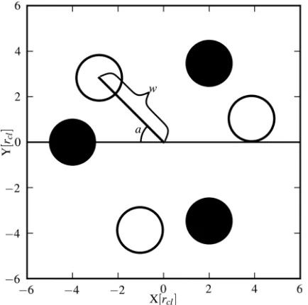
We now investigate the MHD interaction of a shock with three closely spaced clouds which are arranged to form the vertices of an equilateral triangle (see Fig.18). The centroid of the triangle is located at the origin of the computational grid and the exact arrangement is defined by the angle between the vector to the most upstream cloud and the (negative) x-axis and the length of this vector (so distributionw4a30has the most upstream cloud located at (x,y)₌ (₋4cos 30◦_{, 4sin 30}◦_{) =(−3.46, 2)). The most upstream} cloud is referred to as ‘cld1’. The next cloud clockwise, referred to as ‘cld2’, will be the one that is behind (directly or with some

at University of Leeds on January 22, 2015

http://mnras.oxfordjournals.org/

Figure 18. Illustrations of the cloud positions in 3-cloud simulations. Two

particular arrangements are shown:s3w4a0(with the clouds indicated by the

filled circles) ands3w4a45(with the clouds indicated by the open circles).

lateral offset) ‘cld1’. The final cloud, ‘cld3’, is then located off to the side.

A compact,w4 arrangement gives a side length ofl₌√3_× 4₌6.93rcl for the equilateral triangle. If considered as part of

a hexagonal lattice this distribution would give a mass ratio (the ratio of mass in the clouds to the intercloud mass) MR₌9.07. A slightly wider w8arrangement (not considered in this work) givesl₌√3_×8₌13.86rcland MR=2.12. The mass ratio can

be increased by reducing wand by increasing the cloud density contrast,χ.

We now investigate the nature of the interaction with parallel, oblique and perpendicular shocks in turn.

3.3.1 Parallel shocks

The interaction of a shock with three clouds can be thought of as being similar to a two-cloud scenario, but with the addition of a ‘modifier’ cloud. Fig.19shows the nature of the interaction for a relatively compact arrangement of clouds. When clouds are placed further apart the morphology of the interaction increasingly resembles eitherw4a0 orw4a60, except when the orientation is such that the clouds line up.

As with the previous two-cloud simulations, the nature of the three-cloud interaction depends on the relative positioning of the clouds. In Fig.19(a), we see that the ‘flux rope’ from cld1 passes in between the two downstream clouds and completely detaches. In addition, an interesting low-β, low-momentum region forms near the inside ‘wing’ of the downstream clouds. Rotating the cloud distribution to break the lateral symmetry we observe that the ‘flux ropes’ of two of the clouds may merge (as seen in simulations

w4a15andw4a45in Figs19b and d). The merging of flux ropes was previously seen in the two-cloud simulation w2o8shown in Fig.2(d). The location of the third cloud influences the sections of ‘flux rope’ associated with individual clouds but the merged part looks the same. Finally, when cld2 falls directly into the ‘flux rope’ of cld1 (as seen in simulation w4a30in Fig. 19c), the resulting ‘flux rope’ appears very similar to that in the two-cloud simulation

Figure 19. Snapshots att=4tccof various three-cloud simulations with

parallel magnetic fields (β0=1.13). Individual clouds are labelled and the

insert shows the initial cloud arrangement in each case. Only the orientation of the cloud arrangement is changed in these cases.

at University of Leeds on January 22, 2015

http://mnras.oxfordjournals.org/

changed by the presence of the third cloud.

The time evolution of simulationw4a15is shown in Fig.20. In this simulation the strongest interaction occurs between those clouds with the smallest difference in their lateral positions (cld1 and cld2 in this case). Compared to cld2, cld3 is able to retain a broadly symmetric structure for longer, with the only significant deviations byt₌3tccbeing to its tail. After this time, cld3 becomes

increasingly asymmetric in appearance. Att₌ 6tcc, cld2 has a

circular core and a tail of stripped material extending from its outside edge. Such a tail only occurs when a downstream cloud is in the ‘wings’ of an upstream cloud.

To better understand the nature of the interactions between clouds in the three-cloud simulations we now look at the evolution of the mass of the core region of each cloud and each cloud’s density. We define cloud cores as circular regions with an average den-sityρ > ρcrit=120ρamb(i.e. a 20 per cent increase on the initial

cloud density). Fig.21shows the evolution of the core mass in single-cloud simulations and in the three-cloud simulations shown in Fig.19. The core mass rises rapidly as each cloud is compressed and abruptly plateaus once 100 per cent of the cloud material is above the density threshold. This takes roughly one cloud-crushing time-scale by definition. Subsequent re-expansion of each cloud causes the core mass to decrease (in the single-cloud case the core mass decreases to_≈0.5mclbyt≈2tcc). In many cases the

subse-quent behaviour is oscillatory as the cloud cycles through phases of expansion and contraction, though a steady decline in the core mass is the dominant trend as material from the cloud mixes in with the ambient flow (ultimately the cloud density becomes equal to the post-shock density).

In many simulations the cloud fragments into multiple cores. When this happens the mass of the largest fragment is shown by the solid lines in Fig.21while the sum of the mass of all fragments is shown by the dotted lines. Any overlapping cores are merged into a single fragment. We find that this analysis is dependent on the resolution adopted in the simulations. As shown in the top panel of Fig.21, a lower resolution simulation diverges from a higher resolution simulation att_≈3tcc. Therefore, we only consider

high-resolution runs in this analysis (differences due to the high-resolution can be delayed by choosing a lower density threshold,ρcrit). In the

high-resolution single-cloud case, the core splits into two fragments att

≈5tcc, both of which dip belowρcritatt≈6.5tcc(causing the core

mass shown in Fig.21a to drop to zero). Subsequent compression brings material above the density threshold again byt_≈7tcc.

Since cld1 is not downstream of any other cloud, it evolves simi-larly to an isolated cloud and fragments att_≈4.5tcc(see Fig.21b).

Fragmentation of cld1 is slightly suppressed in simulationw4a60

because of the presence of the other clouds alongside. However, subsequent oscillations in the core mass of cld1 due to expansion and contraction of the cloud appear to be much weaker compared to the single-cloud case, indicating that the presence of the other clouds is again being felt. Att₌9tcc, 0.4mclremains in the

com-bined fragments of cld1. The exception to this is simulationw4a30, where the interaction of cld1 with cld2 pushes the average density of cld1 down to 70ρamb(i.e. below the density threshold for

iden-tification of material as ‘core’). The average density of cld1 in the other simulations is_≈90ρambat this time, and for simulations with

an isolated cloud it is at_≈100ρamb.

Various types of interaction show up in the behaviour of the core mass of ‘cld2’. Simulationsw4a0 and w4a15are noticeable for the large mass fraction which remains in the core and the lack of significant fragmentation. In both these simulations cld2 is on the

Figure 20. The time evolution of the three-cloud simulations3w4a15with

a parallel magnetic field (β0=1.13). The logarithmic density and magnetic

field evolution are shown at timest=2.2, 3.0, 4.7, 6.3 and 7.9tcc(top to

bottom). The contour shows the ‘flux rope’ (β <1 andρ|u|<0.5×ρ|u|_ps).

at University of Leeds on January 22, 2015

http://mnras.oxfordjournals.org/

Figure 21. Evolution of the core mass (see text) for (a) single cloud sim-ulations at two different resolutions, and for (b) cld1, (c) cld2 and (d) cld3 in high-resolution three-cloud simulations. In each case the solid line repre-sents the main fragment and the dashed line shows the sum of all fragments.

Thet=0 time for each cloud starts when the shock first reaches the cloud.

Figure 22. Evolution of the density in cld2 in some of the three-cloud simulations. The average density within cld2 is shown by the solid line and the region between the 25th and 75th percentiles is shaded.

‘outside’ edge of the distribution, and the average density of cld2 is similar to that of the single-cloud case. In contrast, the average density of cld2 is lower (and thus there is less mass above threshold) in simulationsw4a45andw4a60. The cores also fragment in these cases. In these simulations cld2 is notable for being in the ‘middle’ of the cloud distributions. Fig.19shows that when cld2 is ‘outside’, it is longer and narrower, whereas when it is in the ‘middle’, it is wider and shorter.

Fig.21 shows that the average core mass of cld3 at late times is similar to or slightly higher than that of an isolated cloud (note that the symmetry of simulationw4a60means that cld3 behaves identically to cld1, while the symmetry of simulationw4a0means that cld3 is identical to cld2). Very little fragmentation is seen in cld3 in any of the simulations, and in particular in simulationw4a0where cld2 is directly alongside it. In general the further downstream cld3 is, the more mass is contained in the core, though this variation is quite small and is somewhat time dependent.

Fig. 22shows the evolution of the density in cld2 in three of the three-cloud simulations. We see that as various shocks pass through cld2 (the transmitted shock is the main one, but shocks also propagate inwards from the sides and back of the cloud), the average density increases by a factor of 3–4. Re-expansion starts aftert_≈

1tccand the density drops reaching a local minimum att≈2tcc.

The density then increases slightly due to compression from the ram pressure of the flow as the cloud is accelerated downstream. The density steadily decreases fromt_≈3tccas the acceleration subsides

and as material is stripped away. In simulations3w4a30, cld2 lies in the ‘flux rope’ of cld1 and is largely shielded from the flow. As a consequence it does not experience a period of re-compression at

t_≈3tcc, but neither does it experience strong stripping by the flow.

Att_≈4tcc, cld1 collides with cld2 and the density of cld2 steadily

increases up tot₌9tcc.

Fig.23shows that the evolution ofβin the material of cld1 and cld3 is largely independent of the cloud arrangement. However, this is not the case for cld2, where clear differences can be seen between simulations in the second and third panels of Fig.23. However, this is hardly surprising, since cld2 is variously located in the ‘flux rope’ of cld1 in simulationw4a30, in the ‘wings’ of cld1 in simulations

w4a15andw4a45, in the ‘outside’ flow in simulationw4a0and in the ‘inside’ flow in simulationw4a60. The presence of a third cloud appears to modify the behaviour seen in Fig.14– specificallyβis higher when cld2 is between cld1 and cld3 (as in simulationsw4a45

andw4a60).

at University of Leeds on January 22, 2015

http://mnras.oxfordjournals.org/

Figure 23. The time evolution of theβdistributions for different clouds in

high-resolution (R128) three-cloud simulations with parallel magnetic fields

and a pre-shockβ=1.13. The solid line shows the median value and the

area between the 25th and 75th percentiles is shaded.

3.3.2 Oblique shocks

We now study the interaction of three-cloud distributions with an oblique shock (θ0=15◦). Fig.24shows the resulting morphology

att₌4tcc. An additional simulation with a negative orientation

angle is also included (simulationw4a-30). In thew4a-30andw4a0

simulations, the modifier cloud is cld2,5_{but otherwise it is cld3. A}

two-stage process occurs: first, cld1 interacts (as in the two-cloud case) with the nearest cloud along the flow, then these clouds jointly interact with the third cloud. For instance, simulationw4a-30in Fig.24(a) can be deconstructed as cld1 and cld3 interacting as in simulationw0o8in Fig.5, and then the resulting combined ‘clump’ interacting with cld2 as in simulationw4o-4in Fig.4. Similarly, simulationw4a60in Fig.24(f) shows cld1 and cld2 interacting as in simulationw4o4, and then together interacting with cld3 as in simulationw4o0(compare Fig.24a with Fig.4d). The secondary interaction can also be categorized in terms of a ‘width’ and an ‘offset’. In the three-cloud simulations studied, it appears that the appropriate width is the average ‘width’ between the combined clump and the third cloud, while the appropriate offset is between the more upstream of the two clouds interacting in the first stage and the third cloud with which they interact in the second stage.6

Note that the secondary interaction has a greater effective ‘width’ than the two-cloud cases considered in Section 3.2. This means that the separation at closest approach is greater and that a secondary collision between the combined clump and the third cloud does not occur. However, otherwise the morphologies are roughly equivalent. Fig.25shows the time evolution of simulations3w4a-30while Fig.26shows the time evolution of simulations3w4a45. In simula-tions3w4a-30, cld1 is initially at the bottom left of the distribution, cld2 is at the top right and cld3 is at the bottom right (see also Fig. 24a). As the shock sweeps over, cld1 moves towards cld3 which is in the lee of cld1. cld1 engulfs cld3 byt_∼4tcc, and cld3

is then confined by the magnetic field threaded through cld1. In contrast, cld2 evolves in a relatively isolated way. The flow tries to force its way between cld1/3 and cld2, but the field lines between these two regions prevent this. In contrast, in simulations3w4a45

cld1 is initially at the top left of the distribution, cld2 is the most downstream cloud and cld3 is at the bottom left (see also Fig.24e). Fig.25shows that cld1 and cld2 interact first, and that cld1 engulfs cld2. Although cld3 is initially upstream of cld2, cld3 lies down-field. Thus as the interaction proceeds, the tension in the field lines created by the flow causes cld3 to accelerate downstream faster than the other clouds.

In the oblique field case cld1 often has very lowβat late times (see Fig.27). Lowβs at late times were previously seen in the top cloud of the two-cloud simulations in Section 3.2 (see simulations

w4o8,w2o8andw0o8in Fig.16). In each case this is caused by the collision of the cloud with a cloud further downstream. Fig.24 re-veals that in the two cases whereβstays higher (simulationsw4a15

andw4a60), cld1 has not collided with another cloud byt₌4tcc. In

simulationw4a15, Fig.24shows cld1 about to squeeze between the two other clouds. cld1 proceeds to move into the ‘shadow’ of cld2, andβin cld1 rapidly grows aftert₌6.5tcc. In simulationw4a60,

cld1 and cld2 accelerate at a similar rate and do not collide (Fig.24

shows these clouds still with significant separation att₌ 4tcc).

However, aftert₌6tcc, as these clouds get close,βdecreases in

cld1.

5_{Naively we expect the switch to happen at an anglea}

≈5◦.

6_{So it is possible to make a priori estimates of these values.}

at University of Leeds on January 22, 2015

http://mnras.oxfordjournals.org/

Figure 24. As Fig.19but for an oblique shock (θ0=15◦,β0=1.13). All

snapshots are att=4tcc.

Figure 25. The time evolution of an oblique shock (θ0=15◦,β0=1.13)

interacting with three clouds (simulations3w4a-30,a= −30◦_).

The evolution of β in the other two clouds does not deviate much from the single-cloud case (see the middle and bottom panels of Fig.27). The only noteworthy behaviour is that cld2 generally has a slightly lowerβ, while cld3 has a slightly higherβ, at late times.β in cld2 is most different from the single-cloud case for simulationw4a0(βbecomes very low byt7tcc), while for cld3

it is simulationw4a30(βbecomes very large att5tcc).

at University of Leeds on January 22, 2015

http://mnras.oxfordjournals.org/

Figure 26. As Fig.25but for simulations3w4a45(θ0=15◦,β0=1.13, a=45◦_).

Figure 27. The evolution of the harmonic mean ofβfor three-cloud sim-ulations with an oblique magnetic field. The top, middle and bottom panels

showβfor cld1, cld2 and cld3, respectively. The time axis is shifted

appro-priately for each cloud. The evolution ofβin isolated clouds is also shown

[for simulations with 32 (R32) and 128 (R128) cells per cloud radius].

3.3.3 Perpendicular shocks

In this section we study the interaction of a perpendicular shock with three closely spaced cylindrical clouds. Fig.28illustrates the range of morphologies which exist att₌4tcc from a variety of

simulations. It reveals that collisions are common. The collisions increase the density of the downstream cloud of the pair and in some cases can last up tot_∼10tcc(cf. Fig.29). In all cases the magnetic

field in the oncoming flow is unable to pass between the clouds. It instead piles up at the upstream side and the field lines then bend around the clumpy region. Clouds either side of the centre of the region then behave like the ‘top’ cloud in the two-cloud oblique simulations (cf. Section 3.2.2).

Fig.29shows the time evolution of simulation s3w4a15. cld1 is initially accelerated towards cld2 and cld3, and at t₌ 4.6tcc

it appears to be poised to squeeze between them. However, the snapshot att₌6.3tcc reveals that this does not happen. Instead,

the field line that cld1 sits on is not able to force its way between cld2 and cld3, and cld1 ends up spreading along it while the field line instead wraps around cld2 and cld3. At the same time, cld2 and cld3 are forced together and mostly merge (they are on similar

at University of Leeds on January 22, 2015

http://mnras.oxfordjournals.org/

Figure 28. As Fig. 19but for a perpendicular shock (β0 = 5.06). All

snapshots are att=4tcc.

field lines). The level of mixing depends on the field strength and the degree of diffusion of material across the field lines. The field lines straighten out at later times as the clouds are accelerated up to the flow speed of the post-shock gas. It is clear that the overall ‘x’-size of the clumpy region is reduced by the field compression in this direction, while the ‘y’-size is reduced by the diffusion of clouds along the field lines.

Fig.30shows the evolution ofβ in the material of cld1, cld2 and cld3 in simulations with a perpendicular field (β0 = 5.06).

In general, we see thatβin cld1 is much lower than the isolated

Figure 29. The time evolution of a perpendicular shock interacting with

three clouds withβ0=5.06 (simulations3w4a15).

single-cloud case, except for simulations3w4a60. This simulation is notable because it is the only one in which cld1 is sufficiently on the ‘outside’ of the distribution that it does not collide with any of the other clouds (see Fig.28). Fig.30also shows that theβin cld2 is similar to but generally lower than the isolated cloud case.βis most variable in simulations3w4a30(in cld2 it is low att₌3.5– 4tccwhen cld1 is compressing cld2, becomes noticeably higher at t₌6tccand then drops again afterwards as it interacts strongly with

cld3). The value ofβin cld3 shows the most difference between simulations. Fors3w4a0 it stays low for most of the simulation

at University of Leeds on January 22, 2015

http://mnras.oxfordjournals.org/