Sequential Auctions in Uncertain Information Settings
Shaheen S. Fatima1 Michael Wooldridge1 Nicholas R. Jennings2
1
Department of Computer Science University of Liverpool, Liverpool L69 3BX, U.K.
{shaheen, mjw}@csc.liv.ac.uk
2
School of Electronics and Computer Science University of Southampton, Southampton SO17 1BJ, U.K.
Abstract. This paper analyzes sequential auctions for private value objects using
second-price sealed-bid rules. Now, the equilibrium bids for such auctions depend on the information uncertainty of the bidders. Specifically, there are three key auction parameters that the bidders could be uncertain about: the valuations of the objects for sale, the number of objects for sale, and the number of participating bidders. We analyse the bidding behaviour for each of these three sources of uncertainty. For each setting, we first find the equilibrium bidding strategies for the individual auctions that comprise a series. Then we analyze the effect of these uncertainties on the computational and economic properties of the equilibrium solution. The former analysis is essential if we want to use software agents to bid on our behalf. The latter is essential because both the auctioneer and the bidders want to know how these uncertainties affect their profits. Thus we compare the outcomes for these settings from the perspective of the bidders (i.e., in terms of their profits), from the perspective of the auctioneer (i.e., in terms of his revenue), and from a global perspective (i.e., in terms of auction efficiency).
1
Introduction
Auctions are now being widely studied as a means of buying/selling resources in multi-agent systems. This is because auctions are not only simple but can also have desirable economic properties, probably the most important of which are their ability to gener-ate high revenues to the seller and also allocgener-ate resources efficiently [13, 2, 15]. Now, in many cases the number of objects to be auctioned is more than one. For such cases, there are two primary types of auctions: combinatorial [12] and sequential [4, 1]. The former are typically used when the objects for sale are all available at the same time, while the latter are used when the objects become available at different points in time. Our paper focuses on sequential auctions. For these, it has been shown that although there is only one object being auctioned at a time, the bidding behaviour for any individual auction strongly depends on the auctions that are yet to be conducted [4, 1].
this is but one source of uncertainty, and there are other auction parameters that the bidders could equally well be uncertain1about. Moreover, these different cases lead to different bidding behaviour and consequently result in different outcomes.
Against this background, our objective is to analyse the bidding behaviour for a range of uncertain information settings. Specifically, we analyse four incomplete infor-mation settings where the bidders are uncertain about:
S1. The other bidders’ valuations for the objects.
S2. The other bidders’ valuations and the number of objects for sale. S3. The other bidders’ valuations and the number of participating bidders.
S4. The other bidders’ valuations, the number of objects for sale, and the number of participating bidders.
For each of these four settings, we first find the equilibrium bidding strategies for the individual auctions that comprise a series. Then we analyze the effect of these uncer-tainties on the computational and economic properties of the equilibrium solution. The former analysis is essential if we want to use software agents to bid on our behalf. The latter is essential because both the auctioneer and the bidders want to know how these uncertainties affect their profits. Thus we compare the outcomes for these settings from the perspective of the bidders (i.e., in terms of their profits), from the perspective of the auctioneer (i.e., in terms of his revenue), and from a global perspective (i.e., in terms of auction efficiency).
Our study shows that, provided the bidders pre-compute certain functions (which we define in terms of their common knowledge about the auction parameters) before the auctions begin, the equilibrium bids can be computed in constant time for all the four scenarios. We also show that between the four scenarios,S1yields maximum profit to the bidders, andS4yields maximum revenue. However, the efficiency remains the same in all the scenarios.
The remainder of the paper is organized as follows. Section 2 describes the auction setting. Sections 3 to 6 determine the equilibrium bids for the four information settings. Section 7 discusses related literature, and Section 8 concludes.
2
The Auction Setting
This model is a generalisation of [1], which studies sequential auctions for two private value objects in the above defined settingS1. Here, we generalise this model tom >2 objects and also analyse it in three different information settings. There aremprivate value objects for sale. Each object is sold in a separate auction using the second-price sealed-bid rules and the auctions are held sequentially. There arenrisk neutral bidders. The valuations for themobjects are independently and identically distributed across the bidders. LetVj : R+ → [0,1](1 ≤ j ≤ m) denote the probability distribution function for the valuation for objectj.
1These other uncertainties have been studied, but mostly for single object auctions – as in [8].
The sequential auctions are conducted as follows. The first object is sold in a second-price sealed bid auction. There arenbidders for this auction. The winning bid for the first auction is announced at the end of the auction. Each bidder needs a single object. Thus the winning bidder for an auction does not participate in any of the subsequent auctions. All the losing bidders for an auction go to the next auction. This process repeats for each of them objects. In other words, the bidders continue to bid in the auctions only until they win an object. Thus, if there arenbidders in the first auction, then there aren−1bidders for the second,n−2for the third, and so on. In general, there aren−j+ 1bidders for auctionj(1≤j≤m).
Given this context, we analyse the four different incomplete information settingsS1, S2,S3, andS4defined in Section 1. Note that a bidder’s uncertainty about the others’ valuations is common to all the settings. The auctions are conducted as follows. To begin, the p.d.fsVj (1≤j ≤m) are common knowledge to all the bidders. However,
each bidder draws his private value signal for auctionjafter the end of auctionj−1. Thus, although the p.d.fs for all the objects are initially known to all the bidders, a bidder comes to know his valuation for auctionjonly just before the auction begins.
In more detail, the auctions are held as follows: i) All the bidders draw their private value signals for auction 1 from the p.d.f.V1. ii) Auction 1 is held using the second-price sealed-bid rules; at the end of the auction, the object is allocated to the winning bidder. iii) The winning bidder for auction 1 leaves (because each bidder has unit demand) and the remaining bidders go to the next auction. iv) For the next auction, the bidders draw their private value signals (signals for auction1≤j≤mare drawn from the p.d.f.Vj).
v) Steps ii to iv are repeated for each of the remaining objects.
Note that the private values for our model are not correlated across themobjects. Such correlations would occur if the value for objectj= 2, . . . , mcan be determined on the basis of the value for object k < j. However, our present work focuses on mdissimilar objects, where such a direct relation between the objects may not exist. Hence, for our analysis, the different objects have different distribution functions.
3
Equilibrium bids for scenario
S
1In this setting, the p.d.fs for the valuations of the objects (i.e.,Vjfor1≤j ≤m), the
number of objects (m), the number of bidders for the first auction (n), and the auction agenda are common knowledge to the bidders.
Since there is more than one auction, a bidder’s bid for an auction depends not only on that auction but also on the profit he expects to get from the future auctions. This profit depends on the number of bidders that participate in the future auctions. Given this, we first determine this profit and then find the equilibrium bids.
chances of winning the first auction, i.e.,β1(1,1, m, n) = 1/n. Recall from Section 2 that if a bidder wins the first auction, he does not participate in the remaining ones.
Now consider the ex-ante probabilityβ1(2,1, m, n), which is the probability that a bidder wins the second auction in the series of auctions from the first to themth one whereβ1(2,1, m, n) = (1−1/n)(1/(n−1)) = 1/n. This is because a bidder can win the second auction if he loses the first one – this has probability(1−1/n). The probability of winning the second auction is1/(n−1). If he wins the second auction then he does not participate in the remaining auctions. In the same way, for1≤y≤m, we getβ1(y,1, m, n)as:
β1(y,1, m, n) = 1 n−y+ 1
y−1 Y
k=1
(1− 1
n−k+ 1) = 1 n−y+ 1
y−1 Y
k=1
n−k n−k+ 1 =
1 n.
In general, forj≤y≤m,β1(j, y, m, n)is given by:
β1(y, j, m, n) = 1 n−y+ 1
y−1 Y
k=j
(1− 1
n−k+ 1) = 1 n−y+ 1
y−1 Y
k=j
n−k n−k+ 1 =
1 n−j+ 1.
(1) Note thatβ1(y, j, m, n)does not depend ony. Intuitively, before the beginning of the jth auction, all bidders are symmetric with respect to winning theyth auction, and there aren−j+ 1bidders left at that point. Hence, each bidder’s probability of winning the yth auction is1/(n−j+ 1). The winner’s expected profit for the(y−1)th auction depends on this probability.
LetEP1(j, m, n)denote the winner’s expected profit for thejth auction in the se-ries ofmauctions withnbidders for the first one. Likewise, letα1(j, m, n)denote a bidder’s ex-ante expected profit from winning any one auction in the series of auctions from thejth (for1≤j≤m) to themth one. This profit is:
α1(j, m, n) =
m
X
y=j
β1(y, j, m, n)EP1(y, m, n) = 1 n−j+ 1
m
X
y=j
EP1(y, m, n).(2)
A definition forEP1(y, m, n)will be given in Theorem 1. Note that since there arem objects,α(m+ 1, m, n) = 0.
Given that the number of objects ismand the number of bidders for the first auction isn, for auctionj,ES1(j, m, n)denotes the expected surplus (surplus is what gets split between the auctioneer and the winning bidder, and it is synonymous with efficiency), andER1(j, m, n)the expected revenue. Finally, fornbidders,E(fjn)andE(snj)
de-note the expected first and second order statistic for the distributionVj, from which the
bidders draw their valuations for auctionj.
Theorem 1. If each auction in a series is conducted using the second price rules, then
the equilibrium for auctionj(1≤j≤m) is:
Proof. In order to find the equilibrium strategies, we begin with the last auction and then reason backwards. Recall that a bidder comes to know his valuationvjjust before
auctionjbegins (i.e., after the previousj−1auctions are over).
Consider auctionm. The number of bidders for this auction isn−m+ 1. Since this is the last auction, the bidding strategies for it are the same as those for a single object auction [13]. Hence we get the following:
EP1(m, m, n) =E(fmn−m+1)−E(s n−m+1
m ) (4)
ES1(m, m, n) =E(fmn−m+1) (5)
ER1(m, m, n) =E(sn−m +1
m ) (6)
Now consider auctionj (1≤ j < m). Consider bidder1and suppose thatb∗ =
maxi6=1bj is the highest competing bid. By biddingxj = vj −α(j + 1, m, n), the
bidder will win ifxj > b∗and lose ifxj < b∗. Now suppose that he bidsz1 < xj. If
xj > z1≥b∗, then he still wins and his profit is stillxj−b∗. Ifb∗> xj > z1, he still loses. But, ifxj> b∗> z1, then he loses whereas if he had bidxjhe would have made
a positive profit. Thus, bidding less thanxj can never increase his profit, but in some
cases it may actually decrease it. A similar argument shows that it is not profitable to bid more thanxj.
Note that, for auctionj,α1(j+ 1, m, n)is a bidder’s expected ex-ante profit from winning a future auction and is therefore constant (i.e., it is the same for all the bidders). Now, this constant may be greater thanvj or less than it. LetCdenote the condition
α1(j+ 1, m, n) < min{vj}. We first analyze the case whereC is true and then the
case whereCis false2.
CTrue: For this case,vj−α1(j+ 1, m, n)is always positive, so the equilibrium bids are:
B1
j(vj) =vj−α(j+ 1, m, n) (7)
Since the equilibrium bid for auctionj decreases byα1(j+ 1, m, n)(relative to a single object auction), the auctioneer’s revenue decreases by the same amount. But the surplus for an auction (which is the sum of the winner’s profit and the auctioneer’s revenue) remains the same as that for a single object auction. Hence, we get the following:
EP1(j, m, n) =E(fn−j +1
j )−E(s n−j+1
j ) +α1(j+ 1, m, n) (8) ES1(j, m, n) =E(fn−j
+1
j ) (9)
ER1(j, m, n) =E(s
n−j+1
j )−α1(j+ 1, m, n) (10)
CFalse: For this case,vj−α1(j+ 1, m, n)may be negative, so the equilibrium bids are:
B1
j(vj) =max{0, vj−α1(j+ 1, m, n)}
Here, the expected surplus, the expected revenue, and the winner’s expected profit for auctionjdepend on the relationship ofα1(j+ 1, m, n)with the valuations for
2
thenbidders. Let the valuations of thenbidders bevn > vn−1>· · ·> v1. Then, there are 3 cases we need to consider depending on this relationship. These cases are as follows: Case 1:α1(j+ 1, m, n)< v1, Case 2:v1< α1(j+ 1, m, n)< v2, Case 3:v2< α1(j+1, m, n). We now analyze each of these cases. In what follows, we letnzdenote the number of bidders whose bid for auctionjis zero.
Consider Case 1. For this case,nz=n. All the bidders bid zero, and so the object
is allocated to a randomly chosen bidder. The winner pays nothing, so the winner’s profit, the surplus, and the revenue are:
EP1(j, m, n) =E(Vj|fn−j
+1
j < α1(j+ 1, m, n)) =E0 ES1(j, m, n) =EP1(j, m, n) =E0
ER1(j, m, n) = 0
Consider Case 2. Herenz =n−1and only one bidder makes a positive bid while
the rest bid zero. Thus, the object is allocated to the bidder with a positive bid. The winner pays nothing because the second highest bid is zero, so the winner’s profit, the surplus, and the revenue are:
EP1(j, m, n) =E(fn−j +1
j |s n−j+1
j < α1(j+ 1, m, n)< fn−j +1
j ) =E1 ES1(j, m, n) =EP1(j, m, n) =E1
ER1(j, m, n) = 0
Consider Case 3. For this case,nz ≤ n−2. Here, the winner pays the second
highest bid so the winner’s profit, the surplus, and the revenue are:
EP1(j, m, n) =E(fn−j +1
j |α1(j+ 1, m, n)< sn−j +1
j )−
E(snj−j+1|α1(j+ 1, m, n)< s
n−j+1
j ) +
α1(j+ 1, m, n) =E2 ES1(j, m, n) =E(fn−j
+1
j |α1(j+ 1, m, n)< sn−j +1
j ) =E2,s
ER1(j, m, n) =E(s
n−j+1
j |α1(j+ 1, m, n)< s
n−j+1
j )−
α1(j+ 1, m, n) =E2,r
By combining these three cases, we get:
EP1(j, m, n) =P0E0+P1E1+P2E2 ES1(j, m, n) =P0E0+P1E1+P2E2,s
ER1(j, m, n) =P2E2,r (11)
where the probabilityP0 = (Vj(α1(j + 1, m, n)))n−j+1, the probabilityP1 = (n−j+ 1)(Vj(α1(j+ 1, m, n)))n−j(1−Vj(α1(j+ 1, m, n)), and the probability P2= 1−P0−P1. Thus, givenα1(j+ 1, m, n), we can findEP1(j, m, n). Hence givenα1(y, m, n)forj+ 1≤y≤m, we can findα1(j, m, n)using Equation 2.
Between Case 1, Case 2, and Case 3, if we assume it is Case 3 (note that under this assumption, the equilibrium bids are as given in Equation 7; soEP1,ES1, andER1 are as given in Equations 8, 9, and 10 respectively) then the expressions for findingEP1 are easier to deal with because we do not have conditional expectations. Moreover, this case is important because, in general, for a large number of bidders, it is quite likely thatP2= 1. This is because asnincreases,E(fjn)−E(snj)decreases [3], so a bidder’s profit from future auctions decreases andα1also decreases. Hence, in the following sections, we will work under the assumption thatP2= 1. We leave the analysis for the other cases (viz., Case 1 and Case 2) as part of future work.
For Case 3, we know from Equations 2 and 8, that the time to findα1(j, m, n)for j = 1isO(m). Sinceα1(j, m, n)is defined recursively, once we findα1(1, m, n)it means that we have already foundα1(j, m, n)for1< j≤m. Hence for auction 1, the time to compute the equilibrium bid given in Equation 7 is alsoO(m). But the time to compute the equilibrium bid for all subsequent auctions isO(1).
4
Equilibrium bids for scenario
S
2This setting is the same asS1except that the bidders are now additionally uncertain about the number of objects for sale. This uncertainty is modelled as follows. We let P Lj denote the probability that auctionj is the last auction. The probabilitiesP Lj
(1 ≤ j ≤ m) are common knowledge to the bidders. Also, P Lm = 1, i.e., all the
bidders know that there are no more than m objects for sale. As before, a bidder’s signal (drawn from the p.d.f.Vjfor auctionj) is his private information.
As before, the equilibrium bids for an auction are obtained using backward reason-ing. However, for this setting, a bidder’s ex-ante probability of winning auctiony in the series fromjtom(denotedβ2(y, j, m, n)) depends on the probability that a given auction is the last one. Thus, we first findβ2(y, j, m, n).
To begin, consider the case where m = 2. For this case, 0 ≤ P L1 ≤ 1and P L2 = 1. Since P L2 = 1(i.e., the second auction is known by all to be the last one),β2(1,1,2, n) = 1/n, andβ2(2,1,2, n) = (1−1/n)(1−P L1)(1/(n−1)). Here (1−1/n)is a bidder’s ex-ante probability of losing auction 1, and(1/(n−1))is his probability of winning auction 2. In general, forj ≤y≤m,β2(j, y, m, n)is:
β2(y, j, m, n) = y−1
Y
k=j
(1−P Lk)(1−1/(n−k+ 1))
×
1
n−y+ 1
= 1
n−j+ 1
y−1 Y
k=j
(1−P Lk) (12)
Letα2(j, m, n)be a bidder’s ex-ante expected profit from winning any one auction in the series from auctionjto auctionmwhere:
α2(j, m, n) =
m
X
y=j
Obviously,α2(m+ 1, m, n) = 0. For this setting, we letB2(·)denote the equilibrium bids,EP2the winner’s profit,ES2 the surplus, andER2 the revenue. The following theorem characterises the equilibrium bids:
Theorem 2. The equilibrium for auctionj(1≤j≤m) is:
B2
j(vj) =vj−α2(j+ 1, m, n) (14) Proof. As per Theorem 1.
It follows from Section 3 that for this equilibrium, the outcome for1≤j≤mis:
EP2(j, m, n) =E(f
n−j+1
j )−E(s n−j+1
j ) +α2(j+ 1, m, n) (15) ES2(j, m, n) =E(f
n−j+1
j ) (16)
ER2(j, m, n) =ES2(j, m, n)−EP2(j, m, n) (17)
Consider the effect ofP Lj on the bidding behaviour for auctionj. We know from
Section 3, that the equilibrium bids for auctionj depend onα1(j+ 1, m, n). As per Equation 2,α1(j+ 1, m, n)depends onβ1(y, j, m, n)(wherej ≤y≤m). Also, since 0≤P Lj ≤1,β2(y, j, m, n)≤β1(y, j, m, n)(see Equations 1 and 12). Consequently, we get:
α2(j, m, n)≤α1(j, m, n) (18)
Hence, from Equations 8 and 15, it follows thatEP2(j, m, n)≤EP1(j, m, n). From Equations 9 and 16 we getES2(j, m, n) = ES1(j, m, n). Also, from Equations 10 and 17 it follows thatER2(j, m, n)≥ER1(j, m, n).
Finally, we look at the time to find the equilibrium bids. We know from Equations 13 and 15, that the time to findα2(1, m, n)isO(m). Hence, for the first auction, the time to compute the equilibrium bid given in Equation14 is alsoO(m). By simply using the values obtained while findingα2(1, m, n), we get the time to get the equilibrium bid as
O(1)for all subsequent auctions.
5
Equilibrium bids for scenario
S
3We know from [8], that for a single object second price auction, the equilibrium bids for the case with a known number of bidders are the same as those for the case of an uncertain number of bidders – i.e., in both cases the bidders bid truthfully. On the basis of this result, we derive the equilibrium bids for sequential second price auctions as follows.
Consider the last auction. Since the equilibrium bids for this auction for the case with a known number of bidders are the same as those for case with an unknown number of bidders [8], the winner’s expected profit, the expected surplus, and the expected revenue are obtained from Equations 4, 5, and 6:
EP3(m, m, n) =
n
X
i=1
P N(m, i)(E(fi
m)−E(s i m))
ES3(m, m, n) =
n
X
i=1
P N(m, i)E(fi m)
ER3(m, m, n) =ES3(m, m, n)−EP3(m, m, n)
We now reason backwards to obtain the bids for the previous auctions. Before doing so, we introduce some notation. LetN be anmelement vector whereNj denotes the
number of bidders in auctionj. Also, letα¯3(j, m, N)denote a bidder’s ex-ante expected profit from winning any one auction in the series from auctionjto auctionmwhen the number of bidders in each of these auctions is as given inN. Letβ¯3(y, j, m, N)be a bidder’s ex-ante probability of winning auctionyin the series of auctions fromjtom, if the number of bidders in each auction is as given inN. For the case where the number of bidders is not known for the individual auctions, we letα3(j, m)denote a bidder’s ex-ante expected profit from winning an auction in the series fromjtom. Then we get the following equations:
¯
β3(y, j, m, N) = 1 Ny
×
y−1 Y
k=j
(1− 1
Nk
)
¯
α3(j, m, N) =
m
X
y=j
¯
β3(y, j, m, N) ¯EP3(y, m, N)
whereα¯3(m+ 1, m, N) = 0andEP¯ 3(y, m, N)is:
¯
EP3(y, m, N) =E(fyNy)−E(sNyy) + ¯α3(y+ 1, m, N)
Since the number of bidders for each auction lies between 1 and n, it follows that α3(m−1, m)is:
n
X
Nm−1=1
n
X
Nm=1
and, in general,α3(j, m)is:
α3(j, m) =
n
X
Nj=1 . . .
n
X
Nm=1
(
m
Y
i=j
P N(i, Ni))×β¯3(i, j, m, N)×EP¯ 3(i, m, N)
Thus, the equilibrium bids for auctionjare the same as those forS1except thatα1in Equation 7 is replaced withα3:
B3
j(vj) =vj−α3(j+ 1, m) (19)
Thus, as in Section 3, we get the following outcome for this scenario:
∀mj=1EP3(j, m) =
n
X
k=1
P N(j, k)×
E(fjk)−E(s k
j) +α3(j+ 1, m)
∀mj=1ES3(j, m) =
n
X
k=1
P N(j, k)×E(fjk)
∀m
j=1ER3(j, m) =ES3(j, m)−ER3(j, m)
We now find the relation betweenα1(j, m, n)andα3(j, m). We know from [3], that for auctionj,E(fn
j)−E(s n
j)is decreasing inn. In order to compareα1andα3, the number of bidders in auction 1 must be the same in both cases – i.e.,P N(1, n) = 1 (and fork < n,P N(1, k) = 0). Then we get:
α1(j, m, n)≥α3(j, m) (20)
Intuitively, this is so because in scenarioS1the number of bidders decreases from one auction to the next, but inS3the number of bidders may increase. And if the number of bidders increases, a bidder’s profit is bound to decrease.
Finally, for this scenario, the number of bidders for an auction lies between 1 and n. Thus, the vectorN can takenm possible values. For a givenN, the time to find
¯
α3(1, m, N)isO(m). Thus, the time to findα3(1, m)isO(mnm)and so is the time to find the equilibrium bid for auction 1. As before, for all remaining auctions, the time taken isO(1).
6
Equilibrium bids for scenario
S
4and 5, it is straightforward to obtain the equilibrium bids forS4as follows:
EP4(m, m, n) = m−1
Y
k=1
(1−P Lk)
×
n
X
i=1
P N(m, i)(E(fmi)−E(s i m))
ES4(m, m, n) = m−1
Y
k=1
(1−P Lk)
×
n
X
i=1
P N(m, i)E(fi m)
ER4(m, m, n) = m−1
Y
k=1
(1−P Lk)
×
n
X
i=1
P N(m, i)E(si m)
¯
β4(y, j, m, N) = y−1
Y
k=j
(1−P Lk)
×β¯3(y, j, m, N) (21)
¯
α4(j, m, N) =
m
X
y=j
¯
β4(y, j, m, N) ¯EP4(y, m, N)
¯
EP4(y, m, N) =
y−1 Y
k=1
(1−P Lk)×EP¯ 3(y, m, N) (22)
α4(j, m) =
n
X
Nj=1 . . .
n
X
Nm=1
(
m
Y
i=j
P N(i, Ni))×β¯4(i, j, m, N)×EP¯ 4(i, m, N)
B4
j(vj) =vj−α4(j+ 1, m) (23)
As in Section 5, we get the following outcome for this scenario:
∀mj=1EP4(j, m) =
n
X
k=1
P N(j, k)×
E(fjk)−E(s k
j) +α4(j+ 1, m)
∀m
j=1ES4(j, m) =
n
X
k=1
P N(j, k)×E(fk j)
∀mj=1ER4(j, m) =ES4(j, m)−ER4(j, m)
Sinceβ¯4(y, j, m, N)≤β¯3(y, j, m, N)(see Equation 21) andEP¯ 4(y, m, N)≤EP¯ 3(y, m, N) (see Equation 22) it follows that:
α4(j, m)≤α3(j, m). (24)
HenceEP4(j, m)≤EP3(j, m)andER4(j, m)≥ER3(j, m). In order to compare α4andα2, we need to takeP N(1, n) = 1. Then, it is straightforward to see that
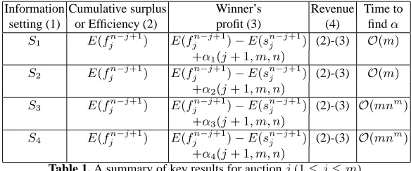
Information Cumulative surplus Winner’s Revenue Time to setting (1) or Efficiency (2) profit (3) (4) findα
S1 E(fn−j +1
j ) E(f
n−j+1
j )−E(s
n−j+1
j ) (2)-(3) O(m) +α1(j+ 1, m, n)
S2 E(fn−j +1
j ) E(f
n−j+1
j )−E(s
n−j+1
j ) (2)-(3) O(m) +α2(j+ 1, m, n)
S3 E(fn−j +1
j ) E(f
n−j+1
j )−E(s
n−j+1
j ) (2)-(3) O(mn m)
+α3(j+ 1, m, n)
S4 E(fn−j +1
j ) E(f
n−j+1
j )−E(s
n−j+1
j ) (2)-(3) O(mn m)
+α4(j+ 1, m, n)
Table 1. A summary of key results for auctionj(1≤j≤m).
So we getEP4(j, m) ≤EP2(j, m, n)andER4(j, m) ≥ ER3(j, m, n). Intuitively, this happens because inS4 the number of bidders from one auction to the next may increase while inS2this number strictly decreases by one. So a bidder’s profit forS4is higher than that forS2.
Finally, as per Sections 4 and 5, we get the time to solve Equation 23 for auction 1 asO(mnm)and for all the remaining auctions asO(1).
7
Related Work
Since Ortega-Reichert’s [11] seminal work on sequential auctions, a considerable amount of research effort has focussed on the subject. This work can be broadly divided into two categories [7, 6]: that which deals with homogeneous objects and that which deals with heterogeneous objects. The analysis of sequential auctions for homogeneous ob-jects is very well developed for the special case where no bidder is interested in more than one unit. Work in this category deals primarily with the study of sale price dynam-ics and shows that even when identical objects are sold in a series, the sale price varies from auction to auction. For instance, Weber [14] showed that in sequential auctions of identical private value objects, the expected sale price is the same for each auction. For sequential auctions with affiliated signals, Milgrom and Weber [10] showed that the expected selling price has a tendency to drift upward in later auctions. Finally, Mc Afee and Vincent [9] considered two identical private value objects and using the second price sealed bid rules, they showed that prices increase in later auctions.
[image:12.612.161.453.65.187.2]Our work differs from the above in that we analyse four different information set-tings, while earlier work on sequential auctions has focused only on uncertainty about the bidders’ valuations for the objects3. By analysing a range of information settings, our work complements and extends earlier work on sequential auctions.
8
Conclusions and future work
This paper analyzes sequential auctions for four different incomplete information set-tings with different sources of uncertainty. For each setting, we obtain the equilibrium bidding strategies and the resulting outcomes for the second price sealed bid rules. We then studied how the different sources of uncertainty affect the computational and the economic properties of the equilibrium solutions.
On the basis of the results given in Table1, we infer the following key conclusions for each individual auction:
1. Sequential auctions are equally efficient in all the four information settings – see Column 2 in Table 1.
2. Between all the scenarios, the winner’s expected profit forS1is the highest – see Equations 18, 20, 24, and 25.
3. Between all the scenarios, the auctioneer’s revenue forS4is the highest – see Equa-tions 18, 20, 24, and 25.
4. Since the revenue for scenarioS2, is higher than that forS1, it is in the auctioneer’s interest not to reveal information regarding which auction is the last one. This leaves the bidders’ uncertain about whether or not there will be any future auctions and forces them to bid higher in a given auction.
5. The time to compute the equilibrium bids for the three scenarios depends on the time to compute the functionsα1,α2,α3andα4(see Equations 3, 14, 19, and 23). But we know from Sections 3 to 6 thatα1,α2,α3, andα4depend on the players’ common knowledge and are independent of their private value signals. Hence they can be computed before the first auction starts and these precomputations can be used when the auctions are run. Using these pre-computed values, it takes constant time to compute the equilibrium bids for each individual auction in each of the four scenarios.
There are several interesting direction for future work. Our present work assumes that the auction agenda is common knowledge to the auctioneer and the bidders. How-ever the agents may equally well be uncertain about the agenda (i.e., the order in which the objects are auctioned). Since the auction outcome strongly depends on the agenda – if we change the agenda, then the outcome changes – we need to consider scenarios with an uncertain agenda and then find the equilibrium bidding strategies. Second, we found the equilibrium bids using the second-price sealed bid rules. The analysis needs to be extended to other auction rules such as English and first-price sealed bid rules. Third, we focused on those scenarios where at least two bidders make a non-zero bid in each auction. We need to extend our analysis to scenarios where this condition is false.
3Even for this specific setting, the equilibrium bids were obtained for a restricted case – see
References
1. D. Bernhardt and D. Scoones. A note on sequential auctions. American Economic Review, 84(3):653–657, 1994.
2. P. Dasgupta and E. Maskin. Efficient auctions. Quarterly Journal of Economics, 115:341– 388, 2000.
3. H. David. Order Statistics. Wiley, New York, 1969.
4. W. Elmaghraby. The importance of ordering in sequential auctions. Management Science, 49(5):673–682, 2003.
5. S. S. Fatima, M. Wooldridge, and N. R. Jennings. Sequential auctions for objects with common and private values. In Fourth International Conference on Autonomous Agents and Multi-Agent Systems, pages 635–642, Utrecht, Netherlands, 2005.
6. P. Klemperer. A survey of auction theory. Journal of Economic Surveys, 13(3):227–286, 1999.
7. V. Krishna. Auction Theory. Academic Press, 2002.
8. D. Levin and E. Ozdenoren. Auctions with uncertain number of bidders. Journal of Eco-nomic Theory, 118:229–251, 2004.
9. R. P. McAfee and D. Vincent. The declining price anomaly. Journal of Economic Theory, 60:191–212, 1993.
10. P. Milgrom and R. J. Weber. A theory of auctions and competitive bidding II. In The Economic Theory of Auctions. Edward Elgar, Cheltenham, U.K, 2000.
11. A. Ortega-Reichert. Models of competitive bidding under uncertainty. Technical Report 8, Stanford University, 1968.
12. T. Sandholm and S. Suri. BOB: Improved winner determination in combinatorial auctions and generalizations. Artificial Intelligence, 145:33–58, 2003.
13. W. Vickrey. Counterspeculation, auctions and competitive sealed tenders. Journal of Fi-nance, 16:8–37, 1961.
14. R. J. Weber. Multiple-object auctions. In R. Engelbrecht-Wiggans, M. Shibik, and R. M. Stark, editors, Auctions, bidding, and contracting: Uses and theory, pages 165–191. New York University Press, 1983.