Cavity flow noise predictions

(1)

AERODYNAMICS & FLIGHT MECHANICS GROUP

Cavity Flow Noise Predictions

by

Xiaoxian Chen, Neil D. Sandham and Xin Zhang

Report No. AFM-07/05

February 2007

COPYRIGHT NOTICE –

All rights reserved. No parts of this publication may be represented, stored in a retrieval system, or transmitted, in any form or by any means, electronic, mechanical, photocopying, recording, or otherwise, without the permission of the Head of the School of Engineering Sciences, University of Southampton, Southampton SO17 1BJ, U.K.

(2)

Cavity Flow Noise Predictions

Final Report for MSTARR DARP

(1 November 2003 to 30 April 2006)

Xiaoxian Chen, Neil D. Sandham and Xin Zhang

February 2007

Aerodynamics and Flight Mechanics Research Group, School of Engineering Sciences

Southampton University

Abstract

(3)

2.1 Introduction of M219 cavity simulations _____________________________________________ 11 2.2 M219 cavity 2-D simulations______________________________________________________ 11 2.2.1 2-D LES simulation___________________________________________________________ 11 2.2.2 2-D DES simulation __________________________________________________________ 13 2.3 M219 cavity 3-D simulations______________________________________________________ 15 2.3.1 3-D LES simulation___________________________________________________________ 15 2.3.2 3-D DES simulation __________________________________________________________ 22 2.4 ReD = 45000 2-D cavity DES simulation _____________________________________________ 24

2.5 ReD = 45000 3-D cavity DES simulations ____________________________________________ 26

2.5.1 Coarse grid _________________________________________________________________ 26 2.5.2 Fine grid ___________________________________________________________________ 28 2.5.3 Comparison _________________________________________________________________ 29

3. Far field Ffowcs Williams-Hawkings (FW-H) predictions ___________________________________ 33

3.1 Implementation of a low storage FW-H solver ________________________________________ 33 3.2 Code validations________________________________________________________________ 34 3.3 Open integration surface sensitivity_________________________________________________ 35 3.3.1 2-D open integration surface ____________________________________________________ 35 3.3.2 3-D open integration surface ____________________________________________________ 39

4. Liner and cavity flow oscillation control __________________________________________________ 42 5. Conclusions __________________________________________________________________________ 47

(4)

1. Introduction

1.1 M219 cavity and ReD=45000 cavity cases

In a project on Turbulence Modelling for Military Application Challenges (TurMMAC) [1] a number of M219 cavity experiments were carried out in the QinetiQ wind tunnels; the resulting experimental pressure data can be used as a benchmark to improve turbulence modelling for flow problems. In this report one of the M219 cavity configurations is utilised, namely the M219 cavity without door and with length (L) of 20 inches, width (W) of 4 inches and depth (D) of 4 inches. The M219 cavity is immersed in a subsonic flow with conditions shown in Table 1.1.1. The M219 cavity is simulated with a newly developed DES code and an existing LES code with improvements in non-reflecting boundary conditions.

Table 1.1.1

Figure 1.1.1: Transducer positions in cavity and on plate. Note that the y and z coordinates correspond to the z and y coordinates used in thecurrent report.

Length (L) 20 (inches)

Depth (D) 4 (inches)

Width (W) 4 (inches)

Mach number (M) 0.85

Total pressure 14.6444 (Psi)

Freestream static pressure 9.1286 (Psi)

Freestream dynamic pressure 4.6190 (Psi)

Reynolds number (Re) 13.353x106 (m-1)

(5)

In the experiment twenty seven kulite transducers were placed on the cavity ceiling, on the front plate and on the rear plate as shown in Figure 1.1.1. Ten unsteady pressure histories with a 6 kHz sample rate at the K20 to K29 transducer positions, fixed on the cavity ceiling

from x/L=0.05 to 0.95 with increment of 0.1D, were provided for comparison. Therefore

overall or band-limited root-mean-square (RMS) pressure distributions can be calculated along the cavity ceiling and be compared with numerical results. There are recommended criteria [1] for a good simulation:

A. Tone frequency prediction error < 5%. B. Tone amplitude prediction error < 5%.

C. Progress achieved in the understanding of issues such as:

• adverse mesh convergence of the computed solution (i.e. mesh divergence);

• influence on RANS solutions of an incomplete separation of scales;

• minimum resolution of scales sufficient for the computation of adequate solutions.

There have been a number of investigations [3-6] on the M219 cavity configuration. Larcheveque [3] used an LES model consisting of a 2nd order spatial scheme, a 2nd order

implicit temporal scheme and a mixed scale turbulence model on a 3.2x106 cell grid. The

predicted mode amplitude errors to the experimental data were -3, -14, 2 and -4 dB

respectively. The 3rd mode was predicted to be dominant while the 2nd mode was dominant in the experimental data. Only the 4th mode frequency was predicted within the 5% error limit. There was an unusual mode prediction at 7.5 kHz. Mendonca etc. [4, 5] used a 2nd order

mixed upwind and central spatial scheme and k-ε turbulent DES model to investigate the

M219 cavity flow on a 1.1x106_{hexahedral cell grid. Details of the temporal scheme were}

not provided. The typical near wall y+ value was about 300. Therefore the near wall physics was not captured. No quantitative comparisons of mode frequency and amplitude were given except the power spectrum densities. Mendonca [5] also gave a comparison between a coarse grid (1.1x106 cells) simulation and a fine grid (2.8x106 cells) simulation. In [4], a band-limited RMS pressure calculation was introduced through a FFT technique. From the presented figures there was no improvement in the RMS pressure prediction on a fine grid. Ashworth [6] used a Fluent DES model with a 2nd order spatial scheme, a 2nd order implicit temporal scheme and a Spalart-Allmaras (S-A) turbulent model to simulate the M219 cavity

flow on a 1.68x106 cell grid. Comparisons between the URANS and the DES predictions

showed that the 2nd mode was missing from the URANS prediction but was captured by the

DES model.

(6)

convergence through two three-dimensional (3-D) grids with different sizes. The flow conditions for the proposed cavity are listed in Table 1.1.2.

Table 1.1.2

1.2 LES and DES models

A. LES model

An LES code, SBLI V3.4, was initially employed to run the M219 cavity flow simulations while the DES model was under development. The numerical model is a compressible flow LES model[8~10]. A 4th_{order central finite-difference scheme is employed for the spatial}

discretization. To improve the nonlinear stability, a split high-order entropy-conserving scheme of Gerritsen and Olsson [11] is used in the Euler equation discretization. In the situation of high Reynolds number flows such as the M219 cavity flow, a weighted five-point filter is applied every ten time steps to strengthen the stability. The time integration scheme is a 3rd order Runge-Kutta scheme [12]. A mixed-scale turbulent model[9] is chosen as sub-grid model in the simulations since it requires no averaging in its execution. This code has been parallelized and optimized for many computing platforms. By placing a buffer-zone combined together with Giles [13] characteristic condition as a non-reflecting boundary condition (NRC) in inflow and outflow regions this code performs better than without buffer zone conditions.

In Cartesian coordinates, the Favre filtered equations are [10],

⎪ ⎪ ⎪ ⎪ ⎩ ⎪ ⎪ ⎪ ⎪ ⎨ ⎧ ∂ ∂ − ∂ ∂ + − ∂ ∂ − = + ∂ ∂ + ∂ ∂ − ∂ ∂ + ∂ ∂ − = ∂ ∂ + ∂ ∂ = ∂ ∂ + ∂ ∂ , ~ ~ ~ ~ ) ~ ~ ( )] ~ ( ~ [ ~ ), ~ ~ ( ~ ~ ~ , 0 ~ j s ij i j ij j s i i i t i i t s ij ij j i j j i i i i x u x u q q x p E u x t E x x p x u u t u x u t τ τ τ τ ρ ρ ρ ρ (1.2.1)

where symbols overbar, tilde and superscripts denote Reynolds, Favre filtered quantities and sub-grid scale quantities respectively. ρ, ui, p, T, Et, τij and τsij are density, velocity

components, pressure, temperature, total energy, viscous stress tensor and sub-grid stress tensor respectively. There are auxiliary relations:

, ~ ~ 2 1 1 ~ , ~ j i

t uu

p E T R p ρ γ ρ + − = = L:D:W 5:1:1

Mach number (M) 0.8

ReD (Re based on D) 45000

(7)

ij s j i j i s ij ij ij S u u u u S µ ρ ρ τ µ τ ~ ~ ~ ~ , ~ ~ _______ = − = = , ~ 3 2 ~ ~ , ~ Pr ~ ~ , ~ Pr ~ ~ k k ij i j j i ij i t s s i i i x u x u x u S x T q x T q ∂ ∂ − ∂ ∂ + ∂ ∂ = ∂ ∂ − = ∂ ∂ − = δ µ µ

where constants γ=1.4, R=287.05, Pr=0.72 and Prt =1. The molecular viscosity µ~∝T0.75

and eddy viscosity _µ~ is modelled by sub-grid (SGS) models. In a mixed-scale SGS model s [9], , | | , ) ˆ~ ~ ( , ~ 1 1 1 2 − − − ⎟⎟ ⎠ ⎞ ⎜⎜ ⎝ ⎛ + ⎟ ⎟ ⎠ ⎞ ⎜ ⎜ ⎝ ⎛ ∆ = − = = S C k T u u k T k C T es s k k es s es MTS s

_ρ

µ

where_∆ ₌₍_∆_x_∆_y_∆_z₎1/3_,_| _| _/ ₂

ij ij S S

S = , S_ij =∂u~_i/∂x_j +∂u~_j/∂x_i , CMTS=0.05,and

CT=10. Advantages of mixed-scale model are no artificial averaging and wall-damping

function required.

B. Spalart-Allmaras (S-A) RANS and DES models

For high Reynolds number flows, the LES model is not a practical tool to simulate near wall physics due to the huge computing cost associated with fine grids. Detached eddy simulation is an alternative way of solving this kind of problems and it uses RANS turbulent models in solid wall area to cut computing cost down. In this project the S-A turbulent model is employed in the DES model and is written as in references [14, 15]:

, ˆ ˆ ) ˆ ( 1 ˆ ˆ ˆ ) 1 ( ˆ ~ 2 1 2 2 2 2 2 1 1 2 1 U f x c x x d f c f c S f c x u t t i b i i t b w w t b i i ∆ + ⎪⎭ ⎪ ⎬ ⎫ ⎪⎩ ⎪ ⎨ ⎧ ⎟⎟ ⎠ ⎞ ⎜⎜ ⎝ ⎛ ∂ ∂ + ⎥ ⎦ ⎤ ⎢ ⎣ ⎡ ∂ ∂ + ∂ ∂ + ⎟ ⎠ ⎞ ⎜ ⎝ ⎛ ⎟ ⎠ ⎞ ⎜ ⎝ ⎛ ₋ − − = ⎟⎟ ⎠ ⎞ ⎜⎜ ⎝ ⎛ ∂ ∂ + ∂ ∂ ν ν ν ν σ ν κ ν ν (1.2.2)

(8)

ft1=0, ft2=0). The kinematic eddy viscosity ν~ is obtained from, s . ˆ , ˆ ~ 3 1 3 3 ν ν χ χ ν χ ν = + = v s c

Other parameters are:

. 1 , , 1 . 0 min , ) ( exp , ˆ ˆ ), ( , 1 ), exp( , / ~ / ~ , , ˆ 1 1 ˆ 2 2 1 1 2 2 2 2 2 2 1 1 2 2 6 2 6 / 1 6 3 6 6 3 2 4 3 2 2 2 1 σ κ ω ω κ ν χ κ ν χ χ b b w t t t t t t t t t t w w w w t t t i j j i ij ij ij v c c c x U g d g d U c g c f d S r r r c r g c g c g f c c f x u x u S d f S S + + = ⎥ ⎦ ⎤ ⎢ ⎣ ⎡ ∆ ∆ = ⎥ ⎦ ⎤ ⎢ ⎣ ⎡ + ∆ − = = − + = ⎟⎟ ⎠ ⎞ ⎜⎜ ⎝ ⎛ + + = − = ∂ ∂ − ∂ ∂ = Ω Ω Ω = ⎟⎟ ⎠ ⎞ ⎜⎜ ⎝ ⎛ + − + =

Constants are cb1=0.1355, σ=2/3, cb2=0.622, κ=0.41, cw2=0.3, cw3=2, cv1=7.1, cv2=5. In the trip

function ft1, dt is defined as the distance from the field point to the trip, which is on a wall, ωt

is the wall vorticity at the trip and ∆x_t is the grid spacing along the wall at the trip. Other constants are ct1=1, ct2=2, ct3=1.1 and ct4=2.

The DES model uses the S-A model with a new distance d~ to replace d: d~=min(d,c_DES∆). ∆ is the maximum distance between the neighbouring cells. A constant cDES=0.65 is defined

for homogeneous turbulence. Therefore away from the cavity flat plates/ceilings the DES model will produce solutions similar to LES with a Smagorinsky sub-grid model.

1.3 SotonCAA code

The SotonCAA code consists of two parts. The first part is for the simulation of acoustic mode propagation through the solution of the modified linearised Euler equations (LEE) [16, 17] while the second part is for CFD flow simulation by solution of the Navies-Stokes (N-S) equations coupled with a DES/S-A turbulence model for sub-grid eddies. In order to maintain a capacity for aeroacoustic noise prediction the code uses high order temporal and spatial schemes to keep wave dissipation and dispersion low. A compact finite-difference scheme (6th order) of Hixon [16] or a 4th order pre-factored scheme [19] is used for spatial derivative calculation. Time integration uses a low storage, low dispersion and dissipation

Runge-Kutta (LDDRK) [20] scheme which is a 4th order 4-6 stage scheme. Other low order

(2nd-3rd) temporal schemes are also available to enable rapid establishment of flow fields, i.e. running to an approximate solution before starting the main calculation. Explicit filtering [21] from 2nd_{to 10}th_{order accuracy is also used to filter out numerical noise and to improve}

(9)

speedup line (straight line), a quasi-linear speedup is achieved and with high number of processors, such as 56 processors, computing efficiency is improved.

Figure 1.3.1: parallel scaling of SotonCAA code

Non-dimensional values of flow variables and coordinates are used in the SotonCAA code. The dimensional reference values are characteristic length L*, free-stream density

ρ

*∞ and

free-stream sound speed

C

*∞. The corresponding non-dimensional values are as follows:

), /( , / , / , / , / , / , / * , / , / , / 2 * * * 2 * * * * * * * * * * * * * * * * * * ∞ ∞ ∞ ∞ ∞ ∞ ∞ ∞ = = = = = = = = = = C p p C R T T C w w C v v C u u L C t t L z z L y y L x x ρ γ ρ ρ ρ

where an asterisk stands for a dimensional value and t and T are non-dimensional time and temperature respectively. R and γ (= Cp/Cv) are the ideal gas constant and the ratio of

specific heats and have values of 287.05 JKg-1K-1and 1.4 respectively. Therefore

non-dimensional free-stream values for flow velocity components, density, pressure and temperature are Mx, My, Mz, 1.0, 1.0/γ and 1.0 where M is Mach number. In this report, the

cavity depth D is chosen as the characteristic length L*.

1.4 Target

(10)

In conjunction with simulation using the SotonCAA DES code and implementation of a low storage Ffowcs Williams-Hawkings (FW-H) solver, other code modifications have also been attempted to extend the capability of the SotonCAA code and to finish the project in time. Not all of these were successful due to limitations of the numerical method (such as high order implicit temporal schemes [29]) or the limitation of the project time (such as

validations of three-dimensional (3-D) open FW-H integration surface due to z length

variations). Cavity flow control is studied through acoustic treatments on inner cavity walls/ceilings. In the analysis of unsteady pressure oscillations on the cavity ceiling, a calculation of the band-limited RMS pressure uses the FFT technique to extract single mode information so that single mode contribution can be studied. Llower and upper limits of the band-width are defined as the mid-point of adjeccent mode frequencies shown in Table 1.4.1. For example the 1st mode band-width is from 76 to 261 Hz for the M219 cavity case. Those mode amplitudes inside each mode band-width are reserved and others are set to null. Pressure history recovered from the spectral space will present mode contributions to the pressure field and the RMS pressure pattern. Through band-limited pressure analyses, mode contribution to the unsteady pressure oscillations would be clear.

Table 1.4.1

Mode 0th 1st 2nd 3rd 4th 5th

M219 cavity case 0 151 Hz 370 Hz 605 Hz 773 Hz 1006 Hz

Re 45000 cavity case 0 524 Hz 1223 Hz 1923 Hz 2622 Hz 3321 Hz

This report is structured as follows. Firstly the M219 cavity flow simulations are described. In Section 2.2 the two-dimensional (2-D) LES and DES simulations are discussed. Three-dimensional (3-D) simulations using LES and DES models are discussed in Section 2.3. In order to complete the project target in time, a low Reynolds number (ReD=45000, M=0.8)

cavity flow case is simulated using the SotonCAA DES/S-A model and results are discussed in Sections 2.4 and 2.5. Section 3 focuses on implementation and application of a low storage FW-H solver and sensitivity tests of the FW-H integration surface. Results of far field cavity flow noise prediction using either low storage or high storage FW-H solver are shown. A 2-D cavity flow oscillation control study is reported in Section 4. Summary of the works and some discussions are given in Section 5. To summarise the cavity cases Table 1.4.2 lists all cases with key parameters included. The cavity length-to-depth-to-width ratio for all cavity cases remains 5:1:1. The total computational domain lengths in the x, y and z directions are shown as TL, TD and TW and the Reynolds number based on the cavity depth D is shown as

ReD.

Table 1.4.2: All cavity cases and key parameters

Model M ReD Grid number TL : TD : TW Total time (sec)

2-D LES 0.85 1358000 7.20x104 11:4 0.159

3-D LES 0.85 1358000 5.74x106 15:7:2 0.151

2-D DES 0.85 1358000 8.17x104 14:6 0.209

3-D DES 0.85 1358000 1.05x106 24:14:2 0.05

2-D DES 0.8 45000 8.09x104 24:14 0.107

3-D DES (coarse) 0.8 45000 1.05x106_24:14:2 _0.088

(11)

2. Cavity near field CFD simulations

2.1 Introduction of M219 cavity simulations

3-D simulation using explicit high order temporal and spatial schemes is an expensive operation in terms of time and computing resources. Therefore a 2-D simulation of the M219 cavity is performed to provide an initial solution with an aim of shortening the flow transient period in the 3-D simulation. The 2-D DES simulation also serves as a validation case to find potential problems during the SotonCAA code development. Although the 2-D simulation is not entirely suitable for DES, results can be used a reference to compare with the 3-D simulation. In addition a sensitivity test of FW-H integration surface placement can also be done in the streamwise (x) and normal (y) directions using results of the 2-D simulation. Simultaneously with the development and validation of the SotonCAA DES code, an existing LES code is utilised to simulate the 2-D and 3-D M219 cavity flows.

2.2 M219 cavity 2-D simulations

2.2.1 2-D LES simulation

Figure 2.2.1.1: A schematic of 2-D grid, unit in D.

Figure 2.2.1.1 shows the 2-D computational domain and stretched grid. SBLI LES code was used to run the 2-D cavity flow simulation on an SGI Origin-3000 computer. Total length in the streamwise direction (along the x axis pointing right) was 11D from x/D=-1 to 10 and total length in the normal direction (along the y axis) was 4D from y/D=0 to 4. Total cell number was 72000. There were 17 cells from y/D=1 to 1.1 and 38 cells from y/D=1 to 1.3 to ensure sufficient grid resolution in the free shear layer. The first cell was 0.005D away from the plate. A characteristic boundary condition and a buffer-zone boundary condition were applied at the inflow and outflow boundaries to filter out reflected acoustic waves. The buffer zone width was 10 cells. A steady flow profile at the inflow boundary was obtained from a turbulent flat plate computation and the turbulent boundary thickness was set at 0.1D at

cavity leading edge according to an estimation of 0.37xRex-0.2 since no experimental

(12)

pressure oscillation is already fully developed from 0.03 sec showing that the self-sustained flow oscillation starts very quickly.

Figure 2.2.1.2: Pressure history at K29.

Table 2.2.1.1: Mode prediction

Modes 1st 2nd 3rd 4th

Rossiter’s formula 159 Hz 371 Hz 582 Hz 794 Hz

Experiment (0.1 sec)

151 Hz 156 dB

370 Hz 158 dB

605 Hz 155dB

773 Hz 144dB 2-D LES 167 Hz _{175 dB} 341 Hz _{171 dB} 506 Hz _{164 dB} 675 Hz _{152 dB}

Table 2.2.1.1 lists the predicted frequencies using a 0.129 sec long pressure data from 0.03 to 0.159 sec with a sample rate of 10 kHz. The Rossiter’s formula [2] can be written as,

, / 1

5 ₁

1 *

κ γ +

−

= ∞

M m D MC

f (2.1)

where f is the resonance frequency and m is the mode number. Constants γ₁=0.25 and

1

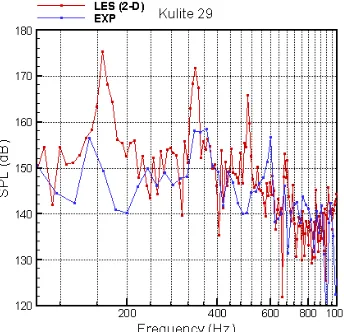
κ =0.57 are phase delay and ratio of the averaged perturbation convective speed to the freestream velocity respectively. It is noticed that the mode frequencies calculated from equation (2.1) are all within 5% of the experimental values. Therefore the Rossiter’s formula predicts this case well. The numerically predicted frequencies are 167, 341, 506 and 675 Hz

at the K29 position and the relative errors compared to the experimental values listed in Table 2.2.1.1 are +11%, -8%, -16% and -13% respectively. The mode frequencies are under predicted except for the 1st mode and all relative errors are over the 5% error limit. The mode amplitudes are also not predicted well. Figure 2.2.1.3 gives a visualisation of the SPL departures. The 1st mode amplitude is 19 dB higher than the experimental one. Form Table

2.2.1.1, the errors of the mode amplitudes are +19, +13, +9 and +8 dB respectively. The

(13)

[image:13.595.94.266.80.246.2]

Figure 2.2.1.3: SPL spectrum at K29. Figure 2.2.1.4: RMS pressure.

Figure 2.2.1.5: Modal RMS pressure.

2.2.2 2-D DES simulation

Figure 2.2.2.1: 2-D computational domain and stretched grid.

As shown in Figure 2.2.2.1 in this simulation the 2-D computational domain was extended so that the buffer-zone conditions were placed further away from the free shear layer, where strong flow nonlinear interaction occurs, because the Giles [13] characteristic condition had

not been implemented in the SotonCAA code. The total length in the x direction was 14D

(14)

81650. At the time of this simulation the grid was extracted from a 3-D grid with a plan to complete the 3-D DES simulation within the time schedule and within the capacity of the computing resources, the y1+, defined as y+ at the first interior grid point near the cavity wall,

was chosen to be about 90 (y1/D=0.003). The solution would not be able to capture near wall

physics such as flow separation as y1+ was not small enough to resolve the viscous sub-layer.

In a similar situation, Mendonca et al. [4, 5] used y1+~300 in their 3-D DES M219 cavity

simulation. As described later in section 2.3, we were able to use y1+~1 for the 3-D DES

M219 cavity flow simulation for 0.05 sec. In this configuration there were 24 cells from

y/D=1 to 1.1 and 45 cells from y/D=1 to 1.3. Boundary conditions were the same as the

previous case. A non-dimensional time step of 2.59x10-4,corresponding to a real time step of 8x10-8sec, was used to advance the solutions.

Figure 2.2.2.2 shows the pressure history at the K29 position. The pressure oscillation is fully developed from 0.089 sec showing that the self-sustained flow oscillation period has started. With a pressure history of 0.12 sec from 0.089 to 0.209 sec, mode predictions are shown in Table 2.2.2.1. Mode errors to the experimental values are +16%, -8%, -9% and -11% for the mode frequencies and +20, +13, +10 and +10 dB for the mode amplitudes respectively. In the 2-D DES computation, the mode prediction, as shown from Figures 2.2.2.3 to 2.2.2.5, are very similar to those of the 2-D LES solutions. However although the DES/S-A model is not actually suitable for a 2-D flow it does give a reasonable prediction of the mode frequencies and at least it validates the SotonCAA code.

Figure 2.2.2.2: Pressure history at K29.

Table 2.2.2.1: Mode frequency comparisons at K29

Experiment

(0.1 sec) 151 Hz 156 dB 158 dB 370 Hz 605 Hz 155dB 773 Hz 144dB

2-D LES 167 Hz _{175 dB} 341 Hz _{171 dB} 506 Hz _{164 dB} 675 Hz _{152 dB}

2-D DES 175 Hz

176 dB

340 Hz 171 dB

518 Hz 165 dB

(15)

Figure 2.2.2.3: SPL spectrum at K29.

Figure 2.2.2.4: RMS pressure. Figure 2.2.2.5: Modal RMS pressure.

2.3 M219 cavity 3-D simulations

2.3.1 3-D LES simulation

The same LES code used in the 2-D simulation was used for a 3-D simulation of the M219 cavity. A periodic boundary condition was applied in the z direction. Based on experiences gained in the previous 2-D cavity flow simulations, a wider computational domain was adopted using a 5.74x106 cell grid. There were 0.88x106 cells (250x80x44) inside the cavity

and 4.86x106 cells (450x150x72) above the cavity. A schematic of 3-D computational

(16)

corresponding to a real time step of 8.7x10-7sec, was used to advance the solutions. The total computational time was 0.151 sec and data were recorded for a 0.1 sec time duration from

0.051 to 0.151 sec. Results of the mode frequency prediction were compared using two

identical time periods, 0.051 to 0.101 sec and 0.101 to 0.151 sec, to show that sufficient computational time was used. Predicted results were also compared with the experimental data with 0.1 sec time duration. Jobs were submitted on the HPCx parallel computer and 128 processors were used with a run time of 12 hours per job.

Figure 2.3.1.1: A schematic of 3-D computational domain.

Figure 2.3.1.2: 2-D slices of grid in x-y plane and in y-z plane (zoom view).

A. Pressure histories and RMS pressure patterns

Figures 2.3.1.3 and 2.3.1.4 show the perturbation pressure histories recorded at three positions along the cavity ceiling. From these data it can be observed that flow oscillation is fully developed from 0.05 sec and the flow field is in a self-sustained oscillation stage. As shown in Figure 2.3.1.5 the pressure fluctuation level reaches its maximum at the rear cavity wall. There are other two features in Figure 2.3.1.5. In comparison with the experimental

RMS pressure (black line), the LES values are higher (by 0 to 1700 Pa) with large

differences in the near wall regions. Inspection of the flow fields finds two flow vortices in the middle of the front and rear walls and their movements have large impacts on the pressure fluctuations around the cavity corners, resulting in the higher RMS pressure. In

comparison with the LES data for two identical periods (0.051 to 0.101 sec and 0.101 to

0.151 sec) no apparent differences are observed suggesting current pressure oscillations are

well developed after 0.051 sec and no further computation beyond 0.151 sec would be

(17)

[image:17.595.83.280.500.678.2]

Figure 2.3.1.3: Pressure history at K21 (x/L=0.15) and K25 (x/L=0.55).

Figure 2.3.1.4: Pressure history at K29 (x/L=0.95). Figure 2.3.1.5: RMS pressure.

Figure 2.3.1.6: Modal RMS pressure (exp). Figure 2.3.1.7: Modal RMS pressure.

In Figures 2.3.1.6 and 2.3.1.7 the mode contributions to the RMS pressure are illustrated. For

the experimental RMS pressure contributions, the 2nd mode contributes the most.

(18)

fixed at x/L=0.05 and 0.95 and for the 4th mode there are four peaks located at x/L=0.05, 0.25, 0.55 and 0.95. In the LES simulation the RMS peaks are determined by their mode number and it is not necessary to have a peak at x/L=0.05, such as in the patterns of the 3rd and 4th

modes. The 1st mode has a major impact on the whole pattern. In comparison to the

experimental pattern the simulation of the 1st mode is poor, resulting in higher RMS pressure distribution.

B. SPL comparison at cavity ceiling

In comparison with experimental data at the K29 position, as shown in Table 2.3.1.1, the LES under-predicts the mode frequency in first three modes and the errors to the experimental data are -13%, -10%, -9% and +3% respectively. Inadequate computing time may be a reason for the unsatisfied mode frequency prediction especially for the 1st mode, as its accurate prediction should require long integration time. However comparisons in two identical time periods have shown sufficient integration time for the prediction, this may not be the reason for the 2nd and 3rd modes and should be explored in future. For the mode amplitude prediction the 3-D LES prediction has a significant improvement over the 2-D LES prediction. The errors to the experimental data are +8, +2, +2 and +5 dB respectively. Compared to the 2-D results the SPL improvements are 11, 9, 7 and 3 dB respectively. The mode amplitude prediction can generally be regarded as good although the dominant mode is not the 2nd mode, which is a common problem in current numerical simulations [3-6].

151 Hz 156 dB

370 Hz 158 dB

605 Hz 155dB

773 Hz 144dB

2-D LES 167 Hz

175 dB

341 Hz 171 dB

506 Hz 164 dB

675 Hz 152 dB

Figures 2.3.1.8 to 2.3.1.17 show the SPL comparisons between the LES results and the experimental data (left-hand figure) and two LES results for the two identical periods (right-hand figure) at the cavity ceiling. For mode predictions at all positions from K20 to K29, the LES under-predicts the 1st modes by 20 Hz but over-predicts the amplitude by 8 dB. For the 2nd mode, the prediction (332 Hz at seven out of ten positions) under-predicts the mode

frequency by 38 Hz and the amplitude differences are between 0 to 5 dB with maximum

value at the K26 position. For the 3rd_{mode, the mode frequency prediction is lowered by 52}

(19)

frequencies, it can be observed from figures 2.3.1.8 to 2.3.1.17 that the LES predictions match the experimental data quite well.

Figure 2.3.1.8: SPL spectrum at K20 (x/L=0.05).

(20)

Figure 2.3.1.11: SPL spectrum at K23 (x/L=0.35).

Figure 2.3.1.12: SPL spectrum at K24 (x/L=0.45).

(21)

(22)

[image:22.595.212.384.292.457.2]

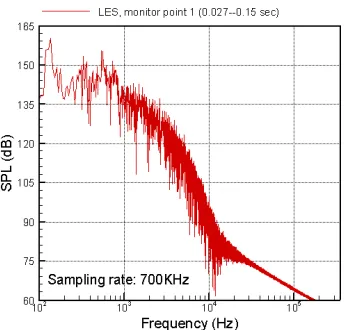
Figure 2.3.1.18: SPL spectrum at x/L=0.5, y/D=1.0, z/D=1.5 (Mid-cavity).

This LES simulation also has pressure recordings at a high sampling rate of 700 kHz at two monitored positions. Figure 2.3.1.18 shows a SPL spectrum at a position in the shear layer (middle of the cavity) and there is no dominant amplitude peak in high frequency range over 1 kHz in this LES simulation as compared to the one predicted at 7 kHz in one published paper [3], which is now believed to have been a numerical artifact.

To conclude the comparison shows that the mode predictions in both periods are almost the same. Therefore there is no need to continue the computation for a longer period. In comparison with the experimental data, reasonable predictions of the modes are observed except for the 1st mode amplitude. This departure from experimental results is consistent with other numerical simulations [4-6].

2.3.2 3-D DES simulation

A schematic of the 3-D mesh is shown in Figure 2.3.2.1. The total cell number was 1.05x106 and the minimum cell volume size was 0.0006D (x) • 0.0002D (y) • 0.006D (z). There were 30 cells clustered in a 0.1D space near the flat plate to ensure y+ ~ 1 and 37 cells from

y/D=1.0 to 1.3 to ensure enough grid resolution in the free shear layer. It was possible to

(23)

processors. Boundary conditions and inflow turbulent profile were the same as those used in the 3-D LES simulation. A fine grid (4.2x106) was established but could not be used in the M219 cavity flow simulation due to insufficient computing power and project time constraint.

[image:23.595.93.518.307.699.2]

Figure 2.3.2.1: 2-D grid slices. (a) x-y plane； (b) y-z plane (zoom view).

151 Hz 156 dB

370 Hz 158 dB

605 Hz 155dB

773 Hz 144dB

3-D DES 145 Hz _{173 dB} 378 Hz _{158 dB} 524 Hz _{150 dB} 669 Hz _{149 dB}

Figure 2.3.2.2: Perturbation pressure history. Figure 2.3.2.3: FFT analysis.

As shown in Figure 2.3.2.2 the pressure oscillation at the K29 position develops after 0.02

sec and only narrowband frequencies can be observed. Table 2.3.2.1 shows the mode

(24)

period only the 2nd mode frequency prediction seems better than the LES results. After 0.05

sec integration time the flow solutions are transferred back to the Iridis2 parallel computer at the Southampton University and the simulation was continued using 56 processors for a period of five months. It Apoears from a zoom view of the streamwise velocity contours shown in Figure 2.3.2.6 that the broadband turbulent features have not developed. Figures 2.3.2.3 to 2.3.2.5 show the mode FFT analysis and the RMS pressure at the cavity ceiling. They all indicate an initial stage of the self-sustained flow oscillations as only the 1st mode is predominant and the 2nd_{mode and higher modes are not properly developed.}

Figure 2.3.2.6: Instantaneous u velocity (zoom view).

2.4 Re_D = 45000 2-D cavity DES simulation

As stated in the introduction section, low Reynolds number 2-D/3-D cavity flows (ReD=45000, M=0.8) were simulated owing to three factors: limitation of the computing

power, y1+ (∼1) requirement and short project time. During the project, 3-D coarse grid and

fine grid cases were studied to address the issue of grid sensitivity.

(25)

number was 80940. Again the computational domain was enlarged in both directions so that the buffer-zone conditions were placed further away from the free shear layer. In this simulation no inflow turbulent profile was provided. An estimation suggested that the starting point of the computational domain at x/D=-4.3 would produce a 0.1D boundary layer thickness at the cavity edge (at x/D=1.0). The y1

+ _{was 1.0 (y}

1/D=0.0037) in the flat plate. At

the flat plate there were 19 cells from y/D=1 to 1.1 and 37 cells from y/D=1 to 1.3. The same boundary conditions were applied as the previous 2-D DES case. Unsteady disturbances were not added in the inflow profile in the boundary layer upstream of the cavity. A non-dimensional time step of 2.23x10-4,corresponding to a real time step of 2x10-8 sec, was used to advance the solutions.

Figure 2.4.1: Computational domain and stretched grid.

[image:25.595.205.402.415.590.2]

Figure 2.4.2: Pressure history at K29.

Table 2.4.1: Mode frequency comparisons at K29

2-D DES 546 Hz

152 dB

1127 Hz 148 dB

1690 Hz 140 dB

2553 Hz 130 dB

(26)

the DES/S-A model is not suitable for a 2-D cavity it does give a reasonable prediction of the mode frequencies. Compared to the results of Rossiter’s formula, the 1st mode frequency is over-predicted by 4%, the 2nd to 4th mode frequencies are under-predicted by 8%, 12% and 3% respectively. Figures 2.4.4 and 2.4.5 show the RMS pressure and the near field SPL pattern respectively. Compared to the M219 cavity case, the lower Reynolds number flow seems to produce lower RMS pressures on the cavity ceiling. Similar to the M219 2-D DES

simulation the 1st mode has a dominant contribution to the overall RMS pressure pattern

indicating that in the 2-D simulations the 1st_{mode is always over-predicted. It is noticed from}

Figure 2.4.5 that the most intensive flow activity happens in the shear layer close to the rear wall and the rear wall region.

[image:26.595.323.519.224.406.2] [image:26.595.88.266.231.405.2]

Figure 2.4.3: SPL spectrum at K29. Figure 2.4.4: Modal RMS pressure.

Figure 2.4.5: SPL pattern.

2.5 ReD = 45000 3-D cavity DES simulations

2.5.1 Coarse grid

Based on the 2-D fine grid used in Section 2.4 a coarse 3-D grid used half of the cells in the x

and y directions. A 2-D y-z slice of the 3-D computational grid is shown in Figure 2.5.1.1 with a 2-D x-y slice (fine grid) in Figure 2.4.1. The total cell number was 1.05x106 of which 0.117x106 cells were inside the cavity. There were 72 computing blocks with 29x36x14 cells per block. Near the flat plate there were 10 cells from y/D=1 to 1.1 and 19 cells from y/D=1

to 1.3. The first cell was 0.0076D away from the plate. The freestream Mach number,

(27)

0.0254 m and 45000 respectively. The ratio of length-to-depth-to-width remained 5:1:1. The domain length in the x direction was 24.4D, ranging from x/D=-4.4 to 20, and the length in the y direction was 14D, ranging from y/D=0 to 14, and length in the z direction was 2.0D

above the cavity, ranging from z/D=0 to 2. In this simulation no inflow turbulent profile was provided. A buffer-zone boundary condition was placed in the inflow and outflow regions to prevent spurious wave reflections. A periodic condition was applied at the spanwise (z) side computational boundaries. The wall temperature was fixed and the no-slip condition was applied to all cavity inner walls and the flat plates upstream and downstream of the cavity. By using a 3rd order explicit Runge-Kutta temporal scheme, a 4th order optimized compact spatial scheme and a 6th order filter in every three time step, a typical time step was 3.3x10-8

sec. The data sampling rate was 10 kHz.

[image:27.595.347.520.242.414.2] [image:27.595.324.510.447.626.2]

Figure 2.5.1.1: 2-D grid slices. (a) x-y plane. (b) y-z plane (zoom view).

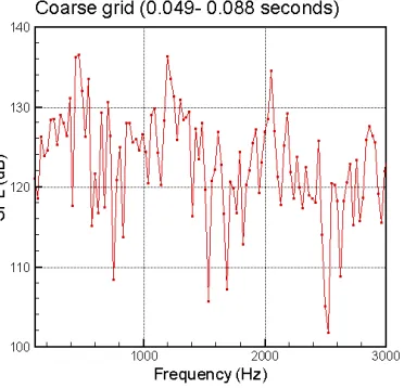
Figure 2.5.1.2: Pressure history at K29. Figure 2.5.1.3: SPL spectrum at K29.

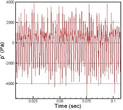
Figure 2.5.1.2 shows the pressure history at the K29 position. The pressure oscillation amplitude falls initially and stays approximately constant after 0.04 sec. Data recorded from

0.049 to 0.088 sec are analysed, with one of the mode analyses and the RMS pressure

distribution along the cavity ceiling shown in Figures 2.5.1.3 to 2.5.1.5. Compared with the 2-D DES case, shown in Figure 2.5.1.4, the RMS pressure prediction is much lower and smoother and the 1st_{mode contributes the most to the overall RMS pressure since two curves}

(28)

mode amplitudes reduced by 11, 14 and 9 dB respectively and the 4th mode amplitude is unchanged. For mode frequencies predicted by the Rossiter’s formula, the 3-D simulation under-predicts the first two modes by 8% and 3% and over-predicts the 3rd and 4th mode by 14% and 12% respectively. The 2nd mode frequency prediction is improved and accurate (in terms of the 5% error limit). The 3-D simulation is important for cavity sound pressure level and RMS pressure predictions. One possible cause for the unreasonably high SPL and RMS pressure predictions in the 2-D results is that in the 2-D domain after flow impingement on the rear wall the high acoustic energy is reflected back to the front wall without much lose creating and maintaining strong cavity flow oscillations. Detailed analyses (in the near future), such as turbulent intensity, shear layer velocity profile etc., should reveal the difference between 2-D and 3-D cavity flow simulations.

2-D DES 560 Hz

150 dB 1120 Hz 149 dB 1682 Hz 140 dB 2562 Hz 130 dB 3-D DES

(coarse grid)

469 Hz 137 dB

1198 Hz 136 dB

2057 Hz 134 dB

2865 Hz 128 dB

2.5.2 Fine grid

The fine grid was the 2-D grid stated in Section 2.4 and extended it along the z direction with 56 cells above the cavity from z/D=0 to 2, with the cavity located from z/D=0.5 to 1.5. The total cell number was 4.08x106 of which a total of 0.453x106 cells were inside the cavity. Therefore the fine grid case had 4 times the number of cells as the coarse grid. There were 72 computing blocks with 57x71x14 cells per block. Near the flat plate there were 19 cells from

(29)

[image:29.595.323.509.218.399.2]

Figure 2.5.2.1 shows the pressure history at the K29 position. The pressure oscillation level stabilizes after 0.028 sec. The pressure data at ten kulite transducer positions from K20 to K29 were recorded from 0.028 to 0.055 sec. To be consistent with the coarse grid case, the pressure data for a 0.021 sec record are analysed. One of FFT results and the RMS pressure distribution along the cavity ceiling are shown in Figures 2.5.2.2 and 2.5.2.3. The amplitudes of the 1st and 2nd modes are 139 and 138 dB respectively. Apart from the first two modes the 3rd_{and 4}th_{modes are not easily identified due to short data length. Consistent with the SPL}

pattern at the K29 position, the modal RMS pressure pattern in the cavity ceiling reveals that the 1st mode is dominant over most of the cavity ceiling.

Figure 2.5.2.1: Pressure history at K29. Figure 2.5.2.2: SPL spectrum at K29.

Figure 2.5.2.3: Modal RMS pressure.

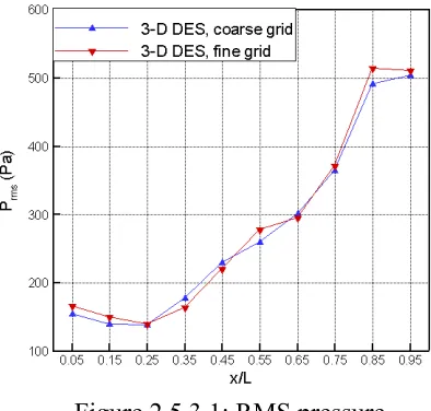
2.5.3 Comparison

A. RMS pattern and mode amplitudes and frequencies

(30)

[image:30.595.204.401.215.403.2]

(Figure 2.5.1.4) is also observed. A detailed comparison of the mode predictions is listed in Table 2.5.3.1. The 1st mode amplitude is the same in both cases but the other three mode amplitudes are higher by 3, 2 and 2 dB respectively for the fine grid. The 2nd mode amplitude is now at the same level as the 1st mode. For mode frequency prediction, the fine grid case under predicts all four modes by 5%, 8%, 9% and 17% compared to the results of the Rossiter’s formula. The modal frequency predictions in fine grid case are worse than the coarse grid case. The only improvement is in the 2nd mode amplitude prediction. It may be assumed that the fine grid resolution resolves the vortex structure in the shear layer and thus improves the prediction of the mode amplitudes especially the 2nd mode.

Figure 2.5.3.1: RMS pressure.

2-D DES 560 Hz

150 dB

1120 Hz 149 dB

1682 Hz 140 dB

2562 Hz 130 dB 3-D DES

(coarse grid)

469 Hz 137 dB

1198 Hz 136 dB

2057 Hz 134 dB

2865 Hz 128 dB 3-D DES

(fine grid)

491 Hz 138 dB

1200 Hz 135 dB

1729 Hz 132 dB

2147 Hz 131 dB

B. Near field SPL pattern, instantaneous pressure and Q criterion

Figures 2.5.3.2 and 2.5.3.3 show the near field SPL pattern. It is observed that the rear wall region experiences the most intensive pressure fluctuations owing to the frequent flow impingements. There is another SPL peak centred in the shear layer and the middle of the cavity illustrating the 2nd mode structure and the second intensive flow activity is in the shear layer. There is no clear difference in terms of the SPL pattern between the coarse and fine grid cases. As illustrated in Figures 2.5.3.4 and 2.5.3.5 the fine grid case gives clear pressure

vortex structures in the shear layer. As the dominant 2nd mode is excited by the flow

(31)

[image:31.595.207.406.492.648.2]

Figure 2.5.3.2: Near field SPL (coarse grid). Figure 2.5.3.3: Near field SPL (fine grid).

Figure 2.5.3.4: Instantaneous pressure (coarse grid).

Figure 2.5.3.5: Instantaneous pressure (fine gird).

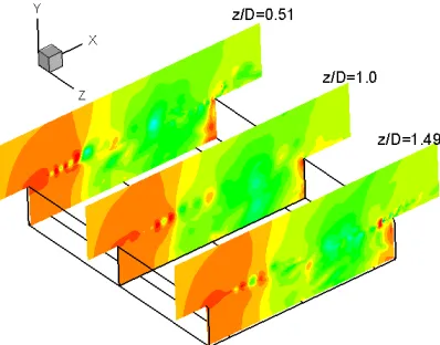
Figures 2.5.3.6 to 2.5.3.9 show the vortex structure through Q criterion [31] in the shear layer region. The fine grid case produces clearer vortex structures, such as small scale vortices in the shear layer. From Figures 2.5.3.8 and 2.5.3.9 the vortex structure variation along the z

(32)

[image:32.595.80.526.86.409.2]

Figure 2.5.3.6: Q criterion (coarse grid). Figure 2.5.3.7: Q criterion (fine grid).

(33)

3. Far field Ffowcs Williams-Hawkings (FW-H) predictions

3.1 Implementation of a low storage FW-H solver

An advanced time method for aeroacoustic predictions has been proposed recently [22]. For the same FW-H formulation developed by Farassat and Succi [23] it has a different implementation compared with a traditional retarded time method [23]. The basic idea is that at a far field observer, acoustic signals emitted from each panel of an integration surface are predicted through an FW-H solver and are gathered at different observer time levels. For an observer at a certain time only part of the acoustic pressure contribution is received. An acoustic pressure prediction will be completed when all signals from the integration surface are received. Far field directivity is calculated at a final stage. As a result of [22], the FW-H solver can now be integrated in the CFD solver and works in a parallel computing environment to provide a far field acoustic pressure prediction in line with the CFD near field prediction. This method does not require hard disk storage and hence is called a low storage FW-H solver. The low storage FW-H solver is essential for far field aeroacoustic predictions in 3-D turbulent flow simulations since usage of hard disk storage would be excessive with previous approaches.

According to [22], acoustic pressure consists of thickness noise p_T′ (x,t), loading noise

) , (x t

p_L′ and quadrupole noisep_Q′ (x,t):

) , ( ) , ( ) , ( ) ,

(x t p x t p x t p x t

p′ = _Q′ + _L′ + _T′ (3.1.1)

where , ) 1 ( )) ( ( ) 1 ( ) ( ) , (

4 ₂ ₃

2 0 2 0 _dS M r M M c M r U M r U U t x p adv r r r n r n n T ⎥ ⎦ ⎤ ⎢ ⎣ ⎡ − − + + − + =

′ ρ ρ

π (3.1.2)

, ) 1 ( )) ( ( ) 1 ( ) 1 ( ) , (

4 ₂ ₃

2

2 2

2 _cr _M dS

M M c M r L M r L L M cr L t x p adv r r r r r M r r r L ⎥ ⎦ ⎤ ⎢ ⎣ ⎡ − − + + − − + − = ′

π (3.1.3)

. )

, (

4 ₃3

2 2 2 1 _dV r K cr K r c K t x p adv Q ⎥⎦ ⎤ ⎢⎣ ⎡ ₊ ₊ = ′

π (3.1.4)

Details of those parameters can be found in [22]. Note that the quadrupole noisep_Q′ (x,t) is not included in this solver. Values of the quadrupole noise p_Q′ (x,t)are small as long as the integration surface is placed away from the strong flow non-linear interaction region (source region), such as free shear layer and viscous boundary layer. Equations (3.1.2) to (3.1.4) are similar to the retarded time formulations except that the surface integral is dropped since the formulation is for an individual panel while in the retarded time method it is for all panels. The advanced time is the time at which a disturbance emitted by a source element y at time t

will reach the observer x. For a subsonic observer velocity it is,

. 1 1 ) ( ) ( | ) ( ) ( | 1 2 2 2 ⎥ ⎥ ⎦ ⎤ ⎢ ⎢ ⎣ ⎡ − − + + + = − + = o o or or adv adv M M t M M c t r t t y t x c t

(34)

3.2 Code validations

[image:34.595.210.387.339.495.2]

Two validations were made. These were un-spinning (m=0) and spinning (m>0) acoustic mode propagations through an unflanged duct. The far field directivity results are shown in Figures 3.2.1 and 3.2.2. Details of the setup can be found in [16, 17] and are not repeated here. To obtain the far field results an oval-shaped 3-D integration surface is established to enclose the source region and near field acoustic data at each panel of the integration surface are collected in time by solving a 2.5D LEE. It should be noted that the low-storage FW-H solver is not suitable for the 2.5D LEE because the acoustic data at the each panel of the integration surface can not be obtained at same time level. Figure 3.2.2 shows that the solver is also correct for spinning-mode far field prediction if near field acoustic data at the integration surface are pre-collected. From both figures it is confirmed that the low storage FW-H solver has the same prediction accuracy as the high storage FW-H solver and matches the analytic solutions. There is no integration surface sensitivity for these two LEE cases since the integration surface is an enclosed surface so that no acoustic information is missed and there is no quadrupole noise included.

Figure 3.2.1: Far field directivity for mode (0, 1) (frequency k=23; M=-0.4, Inlet problem).

[image:34.595.210.386.537.705.2]

(35)

3.3 Open integration surface sensitivity

3.3.1 2-D open integration surface

For a 2-D open integration surface 3-D acoustic data are obtained through data duplication along the z direction. It was reported, on a circular cylinder test [24], that the length of the cylinder had a strong effect on peak noise level and peak amplitude prediction from a cylinder length of 10D was within 2 dB of the experiment. Therefore a 2-D Gaussian pulse case was established as a simplification of the cavity flow case to test the surface sensitivity.

As shown in Figure 3.3.1.1 the rectangular computational domain was 20D long and 20D

high. A uniform mesh was used, containing 478x478 cells to ensure sufficient mesh resolution for monitored data (collected at 0.04 non-dimensional time intervals) to compare with the FW-H prediction. A slip-wall boundary condition was placed at the bottom of the block for the Euler equation simulation and a buffer zone condition, which had a zone width of 20 cell points, was applied at the other three sides to minimize wave reflections. Mean flow properties were taken to be standard: freestream temperature, density, velocity and reference length D were 288.16K, 1.225 kg/m3, 0 m/s and 1.0 m respectively. The initial Gaussian pulse had a strength of 141.86 Pa (0.001*ρ∞C∞2), and was located at x/D=9 and

[image:35.595.217.382.387.553.2]

y/D=2. Positions of the integration surface and three observers are shown in Figure 3.3.1.1 and they are stationary. The disturbance pressure data are collected from these three positions in order to compare with the FW-H predictions.

Figure 3.3.1.1: Illustration of computational domain.

The computation used the Euler equations and 4th-order LDDRK temporal integration

scheme, 6th-order spatial compact scheme and a 10th-order filter in every time step. Four processors were used to ensure correct parallel implementation. The non-dimensional time step was 0.02, corresponding to a CFL condition of 0.478, and the total time steps were 1800 steps. The history data at each panel of the integration surface, which had 200 panels, were collected at 0.04 non-dimensional time intervals. In the FW-H prediction an approximately

(36)

[image:36.595.90.257.423.584.2] [image:36.595.341.510.425.584.2]

Figure 3.3.1.2: z length sensitivity test. Figure 3.3.1.3: FW-H prediction at observer one.

Figure 3.3.1.2 shows the comparison of FW-H predictions using different integration surface

z lengths. In comparison to CAA results at the observer two shown in Figure 3.3.1.1, a z -length of 20D gives most accurate prediction. It seems that the optimized z length is case dependant since an optimized 10D z-length is found in a circular cylinder case [24]. With a fixed z-length of 20D, shown in Figures 3.3.1.3 to 3.3.1.5, the three FW-H predictions seem smoother than the monitored CAA data. These inconsistencies can be visualized from Figures 3.3.1.6 to 3.3.1.9, which show that the wave reflections are formed at the pulse tails. Therefore the CAA result, which can be improved, is not as good as the FW-H prediction due to the narrow buffer zone width.

(37)

[image:37.595.352.494.93.237.2]

Figure 3.3.1.6: Gaussian pulse at t= 2D/C∞. Figure 3.3.1.7: Gaussian pulse at t=4 D/C∞.

Figure 3.3.1.8: Gaussian pulse at t= 6 D/C∞. Figure 3.3.1.9: Gaussian pulse at t=8 D/C∞.

In comparison with the high storage FW-H solver, this solver is efficient for non-periodic acoustic mode prediction and is part of a CFD flow field prediction procedure, which is user friendly. There is no need to calculate the time variation of the acoustic data as the CFD solver provides those values as well. However, since this solver is integrated into the main CFD solver, the integration surface has to be constructed before time integration, which may cause difficulty in verifying the effectiveness of the integration surfaces. Therefore in conducting integration surface sensitivity tests the high storage FW-H solver is preferred because it is a post-processing activity.

A sensitivity study of open integration surface placement for the 2-D ReD=45000 cavity case

(38)

direction. The far field results at 100 m (centered at cavity rear edge shown in Figure 3.3.1.12) show that a consistent directivity pattern is observed at an observation angle 30<φ<69 degrees, where φ is defined in Figure 3.3.1.12. The maximum SPL difference is 2 dB. The peak SPL value is within the area where the maximum relative difference is 1.6%. The peak SPL value is predicted at 64 degrees.

[image:38.595.209.387.175.329.2]

Figure 3.3.1.10: z length sensitivity.

Figure 3.3.1.11: Comparison of near field SPL.

(39)

Figure 3.3.1.13: Far field FW-H predictions.

3.3.2 3-D open integration surface

For the 3-D cavity cases flow perturbation values at the integration surface outside the computation domain of z/D=0 to 2.0 are obtained through interpolation of the flow values inside the domain according to a periodic flow assumption in the z direction. The sensitivity study of the placement becomes difficult owing to the long integration time. Therefore to study the z-length effects three z-lengths are used in three cavity cases. Based on experience

gained in the 2-D Gaussian pulse and the 2-D ReD=45000 cavity cases, the lengths are

chosen to be 18D, 30D and 37D for the 3-D M219 cavity, ReD=45000 coarse grid and fine

grid cavity cases respectively. Similar results are obtained for the near field FW-H predictions so that only one result from the M219 cavity case is shown. As shown in Figure 3.3.2.1 a perturbation pressure history is recorded from 0.2 to 0.5 sec at a monitoring position

shown in Figure 3.3.1.12. The maximum perturbation pressure has a value of 900 Pa. The

corresponding low storage FW-H prediction is also shown in Figure 3.3.2.2. The predicted time is actually out of the monitored time range so that both monitored and the predicted data are not able to be compared directly. Assuming the pressure has a similar pattern after 0.5 sec

(40)

[image:40.595.328.505.81.259.2] [image:40.595.89.268.89.251.2] [image:40.595.208.402.496.675.2]

Figure 3.3.2.1: Monitored pressure. Figure 3.3.2.2: FW-H prediction.

Figure 3.3.2.3: FW-H prediction (0-0.8 sec).

Figure 3.3.2.4: FW-H prediction (0.08 to 0.11 sec).

Figure 3.3.2.5 shows the current far field directivity predictions, in which observers are

located 100 m away from the cavity rear corner, for the 3-D M219 case. Two curves are

(41)

than 3 kHz. It is observed that the high frequency components do not contribute to the SPL prediction significantly as there is a close match between truncated and non-truncated data from 15 to 110 degree angles. The predicted SPL level is exceptionally high with a maximum value of 156 dB, which is equivalent to a near field prediction. As addressed before the time schedule of this project does not leave room for completion of the simulation so that a correct far field FW-H prediction can be made. Although the SPL level prediction is not correct the directivity peak angle should be correctly predicted and it is 60 and 57 degrees for truncated and non-truncated data. Similar directivity patterns with peak angles near 60 degrees were observed from simulations [25-27], which confirm the result presented here. For the 3-D

ReD=45000 cases Figure 3.3.2.6 shows the far field directivity prediction comparison

between the coarse and fine grids, with the high frequency components truncated after 3 kHz. The SPL level prediction has same problem as in the M219 case, showing the same transient period for the far field directivity prediction. Both coarse and fine grid cases predict a peak angle at 54 degrees which is 10 degree lower in comparison with the prediction of 64 degrees in the 2-D cases. Both cases are not significantly different in terms of directivity shape.

[image:41.595.206.388.296.480.2]

Figure 4.3.2.5: Far field directivity for M219 cavity.

[image:41.595.206.387.513.697.2]

(42)

4. Liner and cavity flow oscillation control

An acoustic liner is implemented numerically as an impedance condition so that the solid wall becomes a ‘soft’ wall where the liner is placed. In the frequency domain, harmonic components of the surface pressure, pˆ , are related to a normal velocity component uˆ by an impedance Z,

u p

Z(ω,θ)= ˆ/ ˆ, (4.1)

where ω is an angular frequency and θ is an incident angle. In reference[28], a reflective wave _u_{ˆ is related to a incident wave}− _u_{ˆ by a parameter}+ _W_ˆ _,

) 1 /( ) 1 ( ˆ / ˆ

ˆ _u _u _Z _Z

W = − + = − + . (4.2)

In the time domain, the convolution process is expressed as:

. ) ( ) ( )

(t W t τ u τ dτ

u +∞ +

∞ − −

∫

−

= (4.3)

By defining a single frequency dependence,

), /

( )

(ω R₀ i X ₁ ω X₁ω

Z = + ₋ + (4.4)

where resistance R0and reactanceX−1/ω+X1ω can be measured through experiments and

acoustic mass X-1 and stiffness X1 can be calculated. Although in real flow situations, such as

the cavity flow, the mode frequency is broadband, the single frequency expression is useful in determining the best frequency of a liner for noise reduction.

The chosen test case is a 2-D DES/S-A ReD=45000 cavity flow case presented in Section 2.4.

In this case a constant depth ceramic tubular liner is chosen, as its best frequency for noise reduction is 1.0 kHz and the cavity dominant mode is the 2nd mode with a frequency of 1.2

kHz. Since the cavity flow frequency is broadband, the broadband impedance condition with mean flow effects included[28] is implemented together with a single-frequency condition. Defining a parameter Wˆ ,

, ) ( ) ( ) ( ) ( 1 2 1 2 1 ˆ ˆ 2 2 ω ω ω ω

ω D i

i Q X i R Z W W = + + = + = −

= (4.5)

where R and X are the resistance and reactance respectively. If the denominator D(iω) assumes form such as (iω-λ1) (iω-λ2)… (iω-λm), the value of Wˆ can be obtained from

measured data. Detailed derivations can be found in[28] and are not repeated here.

The cavity flow oscillation is self-contained and is driven by a flow dynamic process (i.e.

(43)

use of acoustic liners may not in itself achieve a great success, but may provide clues for better control. In the initial stage, the tests are designed to determine how successful the oscillation attenuation can be by using the impedance data (acoustic tube) available and finding a position on the cavity walls/ceilings where the noise attenuation can be effective. The dominant modes for this cavity flow are 1 to 3 which are in a range from 0.5 to 2.0 kHz. Therefore one impedance value corresponding to frequency from 1.0 kHz was used in a single-frequency test and six impedance values corresponding to frequencies from 0.5 to 3.0

kHz were used in the broadband-frequency test. Two liner positions were chosen as shown in Figure 4.1. One of the reasons for choosing these locations was that the rear wall region experiences the strongest pressure fluctuations and the cavity inner walls/ceilings as a whole act like a resonator. The first position (liner 1 case) was at the rear wall and the second (liner 2 case) was at all cavity inner walls/ceilings. The hard wall case was selected as a baseline configuration for comparison. In the analysis, only SPL data on the K29 position were used. The liner and baseline simulations used an existing flow solution and an integration time of 0.0106 sec which covered five periods of the 1st mode.

Figure 4.1: Liner positions in a 2-D cavity.

A. Broadband-frequency impedance

Three comparisons are performed: domain SPL pattern, mode FFT analyses and RMS pressure patterns. Figures 4.2 to 4.4 show the SPL patterns for the baseline and both liner cases. It can be observed that the liner 2 case has better cavity flow oscillation reduction in the near field since the area of large SPL value is obviously reduced to a small area close to the rear cavity wall in comparison with the baseline case. This indicates a reduced strength of acoustic feedback and weaker flow instability excitement in the free shear layer. The liner 1 case is less effective on the flow oscillation reduction because the acoustic treatment is only done at the rear wall and acoustic feedback from the ceiling and the front wall are not affected. In both cases the maximum SPL reduction is 1.3 dB.

(44)

Figure 4.3: Near field SPL: liner 1.

Figure 4.4: Near field SPL: liner 2.

Figure 4.5 shows the mode amplitude results for both liner positions. Compared to the baseline case, in the liner 1 case the first three mode amplitudes are 153, 139 and 141 dB and the mode frequencies are 561, 1028 and 1401 Hz respectively. Mode frequencies are shifted from the baseline frequencies and at the baseline mode frequency positions the amplitudes are equivalent or higher for the 1st_{and 3}rd_{modes and lower for the 2}nd_{mode. Both mode}

(45)

Figure 4.5: Comparison of pressure spectrums. Figure 4.6: RMS pressure.

B. Further study of singe-frequency impedance at 1.0 kHz

The single-frequency impedance study is to find how much noise reduction can be achieved if the system responds to a single-frequency only. This is done numerically assuming a new liner, which has a characteristic of single-frequency response of 1.0 kHz.

[image:45.595.324.521.76.263.2]

Figure 4.7: Near-field SPL: Liner 1 case.

Figure 4.8: Near-field SPL: Liner 2 case.

[image:45.595.87.284.78.253.2]

(46)

SPL value area nearly disappears in the region close to the rear wall in the liner 2 case suggesting weaker cavity flow oscillations in comparison with the corresponding SPL pattern shown in Figure 4.7. In comparison with the broadband-frequency impedance results, the single-frequency impedance has a better noise attenuation effect.

[image:46.595.324.521.147.328.2] [image:46.595.92.290.149.319.2]

Figure 4.9: Comparison of pressure spectrums. Figure 4.10: RMS pressure.

As observed from Figure 4.9, the pressure spectrum analysis shows that the mode

amplitudes are reduced at frequencies less than 2.0 kHz for both liner cases. A better

reduction is observed for the liner 2 case. In the liner 1 case the first two mode amplitude reductions are 2.0 and 3.0 dB and mode frequencies are shifted to 467 and 748 Hz from the original 561 and 1028 Hz respectively. In the liner 2 case, the first two mode amplitude

reductions are 10.0, and 8.0 dB and mode frequencies are shifted to 281 and 748 Hz