Joint Source-Channel Coding for Image Transmission over Underlay Multichannel Cognitive Radio Networks

Rochester Institute of Technology

RIT Scholar Works

Theses

7-2019

Joint Source-Channel Coding for Image

Transmission over Underlay Multichannel

Cognitive Radio Networks

Long Pham

[email protected]

Follow this and additional works at:https://scholarworks.rit.edu/theses

This Thesis is brought to you for free and open access by RIT Scholar Works. It has been accepted for inclusion in Theses by an authorized administrator of RIT Scholar Works. For more information, please [email protected].

Recommended Citation

Joint Source-Channel Coding for Image

Transmission over Underlay Multichannel

Cognitive Radio Networks

Joint Source-Channel Coding for Image

Transmission over Underlay Multichannel

Cognitive Radio Networks

Long T. Pham

July 2019

A Thesis Submitted in Partial Fulfillment

of the Requirements for the Degree of Master of Science

in

Computer Engineering

Joint Source-Channel Coding for Image

Transmission over Underlay Multichannel

Cognitive Radio Networks

Long T. Pham

Committee Approval:

Dr. Andres KwasinskiAdvisor Date Department of Computer Engineering

Dr. Shanchieh Yang Date

Department of Computer Engineering

Acknowledgments

I would like to thank my Thesis Advisor, Dr. Andres Kwasinski, for all his support and guidance, not only with this thesis but also throughout my years at RIT. Without Dr. Kwasinski’s mentorship and direction, none of this is possible. I would also like to thank Dr. Shanchieh Yang and Dr. Panos Markopoulos for being part of my Master’s thesis committee.

I would like to thank all the professors, TAs, and staff members throughout my time here at RIT. I have come a long way since being a freshman thanks to their efforts in teaching me and challenging me to new heights.

I would like to thank fellow class of 2018 graduates, especially the senior design group, for making this college journey of mine all the more fulfilling. I’ve learned so much from them, inside and outside the classrooms.

Abstract

Contents

Signature Sheet i

Acknowledgments ii

Abstract iii

Table of Contents iv

List of Figures vii

List of Tables x

Acronyms xi

1 Introduction 2

2 Background 5

2.1 Cognitive Radio . . . 5

2.1.1 Overview . . . 5

2.1.2 Cross-layer Paradigm . . . 6

2.2 Set Partitioning in Hierarchical Trees . . . 8

2.3 Joint Source-Channel Coding . . . 9

2.4 Unequal Loss Protection . . . 12

CONTENTS

2.4.2 Link Layer Protection . . . 14

3 Previous Work 16 3.1 Unequal Error Protection . . . 16

3.2 Cross-layer Design for ULP in CR Networks . . . 16

3.3 Neural Network Cognitive Engine for Underlay DSA . . . 18

3.4 JSCC for Progressive Transmission of Embedded Source Coders . . . 19

3.5 Cooperative Learning for Reduced Complexity CR . . . 19

4 Proposed Methodology 21 4.1 Overall System Setup . . . 21

4.2 Implementation Details . . . 22

4.2.1 Source Encoder - SPIHT . . . 22

4.2.2 Channel Encoder . . . 24

4.2.3 Rest of System . . . 31

5 Experimental Evaluation 32 5.1 Experimental Setup . . . 32

5.1.1 ELP Test . . . 32

5.2 Results and Analysis . . . 34

5.2.1 SPIHT Encoder . . . 34

5.2.2 Channel Encoder . . . 35

CONTENTS

List of Figures

2.1 Three main DSA paradigms: (a) Interweave (b) Underlay (c) Overlay

[4] . . . 6

2.2 Parent-offspring dependencies in SPIHT [9] . . . 9

2.3 Traditional coding model (top) vs. JSCC (bottom) . . . 10

2.4 An example of Reed-Solomon code . . . 13

2.5 JSCC setup with error protection at the link layer . . . 15

3.1 The hill-climbing algorithm in progress to assign FEC values to differ-ent streams [2] . . . 17

3.2 Implementing ULP for SPIHT bit stream [16] . . . 18

3.3 Progressive transmission of five source packets [18] . . . 20

4.1 End-to-end system setup . . . 21

4.2 Block diagram of the research tool’s usage in this work . . . 23

4.3 Average secondary network throughput under different PN loads [17] 25 4.4 Illustration of an FDD frame [22] . . . 27

4.5 Bits selection from the output SPIHT stream . . . 31

5.1 Original Lena image . . . 33

5.2 Original Goldhill image . . . 33

LIST OF FIGURES

5.4 Comparison of SPIHT encoding efficiencies: (a) with the tool (b) orig-inal code [8] . . . 35 5.5 Comparison of SPIHT encoding efficiencies with the tool (a)

compres-sion ratio 8 (b) comprescompres-sion ratio 40 . . . 36 5.6 Lena’s average code rate selection results for ULP and ELP, codeword

length 14 . . . 39 5.7 Goldhill’s average code rate selection results for ULP and ELP,

code-word length 14 . . . 40 5.8 Barbara’s average code rate selection results for ULP and ELP,

code-word length 14 . . . 41 5.9 Lena’s average P SN R results for ULP, codeword length 14 . . . 42 5.10 Goldhill’s average P SN R results for ULP, codeword length 14 . . . . 43 5.11 Barbara’s average P SN R results for ULP, codeword length 14 . . . . 43 5.12 Lena’s decoded images using ULP with codeword length 14 . . . 44 5.13 Goldhill’s decoded images using ULP with codeword length 14 . . . . 45 5.14 Barbara’s decoded images using ULP with codeword length 14 . . . . 46 5.15 Lena’s average P SN R results for ULP relative to ELP, codeword

length 14 . . . 47 5.16 Goldhill’s average P SN R results for ULP relative to ELP, codeword

length 14 . . . 47 5.17 Barbara’s average P SN R results for ULP relative to ELP, codeword

length 14 . . . 48 5.18 Lena’s average code rate selection results for ULP and ELP, codeword

length 15 . . . 49 5.19 Goldhill’s average code rate selection results for ULP and ELP,

LIST OF FIGURES

5.20 Barbara’s average code rate selection results for ULP and ELP, code-word length 15 . . . 51 5.21 Lena’s average P SN R results for ULP, codeword length 15 . . . 52 5.22 Goldhill’s average P SN R results for ULP, codeword length 14 . . . . 52 5.23 Barbara’s average P SN R results for ULP, codeword length 15 . . . . 53 5.24 Lena’s average P SN R results for ULP relative to ELP, codeword

length 15 . . . 53 5.25 Goldhill’s average P SN R results for ULP relative to ELP, codeword

length 15 . . . 54 5.26 Barbara’s average P SN R results for ULP relative to ELP, codeword

List of Tables

4.1 PN load and secondary network throughput, PN relative throughput change = 2% . . . 26

Acronyms

CR

Cognitive Radio

DSA

Dynamic Spectrum Access

ELP

Equal Loss Protection

FEC

Forward Error Correction

JSCC

Joint Source and Channel Coding

LIP

List of insignificant pixels

LIS

List of insignificant sets

LSP

List of significant pixels

Acronyms

PSNR

Peak-Signal-to-Noise Ratio

RB

Resource Block

RS

Reed-Solomon

SINR

Signal-to-Interference-and-Noise Ratio

SNR

Signal-to-Noise Ratio

SPIHT

Set Partitioning in Hierarchical Trees

ULP

Chapter 1

Introduction

The radio spectrum consists of extremely valuable frequency bands used for many purposes. Telecommunications, in particular, make heavy usage of the electromag-netic waves in this spectrum; not to mention radio broadcasting, communications between aircrafts and ships, radar, and industrial, scientific, and medical (ISM) uses. However, increasing demands in the spectrum, fueled by the ever growing number of connected devices and bandwidth demanding applications, leads to more congestion and interference within the fixed spectrum. Another serious problem is spectrum access in locations where users cannot utilize frequency bands unused by their in-cumbent owners due to strict regulations. A number of techniques have emerged to remedy these issues, among them, cognitive radio (CR).

CHAPTER 1. INTRODUCTION

transmissions.

CHAPTER 1. INTRODUCTION

Chapter 2

Background

2.1

Cognitive Radio

2.1.1 Overview

CHAPTER 2. BACKGROUND

Figure 2.1: Three main DSA paradigms: (a) Interweave (b) Underlay (c) Overlay [4]

As seen in Figure 2.1a, at time slot t1, the secondary user is able to transmit at

frequency band B5 but not in bands B1, B2 or B3; while at the next time slot t2, the

frequency bands B1, B2 or B3 are all available but B5 is not.

However, secondary users need not to find spectrum holes to be able to use the bands; they can be assigned as the secondary network and are allowed to coexist with the primary network, under the premise that the secondary network does not produce excessive interference that can disrupt the operation of the primary network. In Figure 2.1b, the secondary user has to keep its transmit power at a respectable level, but otherwise can use any frequency band, even if it is occupied by a primary user. This is what defines the Underlay DSA paradigm [4, 5], for which as long as the interference limit is kept, secondary users can transmit without the knowledge of the arrivals of the primary user.

2.1.2 Cross-layer Paradigm

re-CHAPTER 2. BACKGROUND

sponsible for high-level APIs and the whole application itself, the Physical layer at the other end of the layer stack is responsible for transmitting and receiving bits over the physical channel. For OSI models, the key aspect is that implementation details of a layer are typically not known by other layers; and that layers only exchange infor-mation with their neighboring layers [6]. The layered structure also allowed modular design for standardization and for layers to develop independently of other layers as newer technologies are deployed. However, its performance in wireless networks is severely limited by the transmission medium, in which the layered architecture is not very effective. For example, TCP/IP’s lack of communication between the link layer (which handles the channel errors), and the transport layer (which performs congestion control) hinders performance in the case of transmission in fading wireless networks [6, 7].

CHAPTER 2. BACKGROUND

2.2

Set Partitioning in Hierarchical Trees

CHAPTER 2. BACKGROUND

Figure 2.2: Parent-offspring dependencies in SPIHT [9]

2.3

Joint Source-Channel Coding

CHAPTER 2. BACKGROUND

Figure 2.3: Traditional coding model (top) vs. JSCC (bottom)

With JSCC, the parameters of the two codecs will be jointly configured as a tandem. Figure 2.3 shows this distinction. The primary goal of the code rate adaptability is to balance distortions from both the source encoder, the ”source coding distortion”

DS, and the channel encoder, the ”channel-induced distortion” DC [11]:

D=DS+DC (2.1)

Let the source signal be denoted as s[n]. It is then sampled, quantized, transmitted, and finally is performed reverse operations as the transmitter side to produce the output signal ˜s[n]. Becauses[n] is sampled, it can be expressed in the following form:

s[n] =

N

X

k=1

skφk(t) k = 1,2, . . . , N (2.2)

CHAPTER 2. BACKGROUND

[11]. The received signal ˜s[n] can be expressed in the same form:

˜

s[n] =

N

X

l=1

˜

slφl(t) l= 1,2, . . . , N (2.3)

With these quantities being defined as well the transmitted symbol duration beingT

and the quantized sample sk being ˆsk, the source coding distortion can be expressed

as follows:

DS =E

" _N X

k=1

(sk−sˆk)2

#

Similarly the channel-induced distortion can be expressed as follows:

DC =E

" _N X

k=1

(ˆsk−s˜k)2

#

CHAPTER 2. BACKGROUND

Once the JSCC system has its rate configured to minimize the end-to-end distortion, it is used to transmit images with the goal of achieving the highest quality possible at the receiver side. From the transmitter to the receiver, an image has to face end-to-end distortion, channel packet loss, and many other factors which cause its quality to decrease. The image is considered to be contaminated with noise, and more noise contamination further decreases image quality, which is commonly measured in PSNR as follows:

P SN R= 10log10

2552

M SE

, (2.4)

where MSE indicates the mean squared-error between the source image and the re-constructed image. Higher PSNR values means lower MSE and thus higher decoded image quality.

2.4

Unequal Loss Protection

hand-in-CHAPTER 2. BACKGROUND

hand with SPIHT (by its nature sorting bits by their significance). Forward Error Correction is performed by giving each message fragment the appropriate amount of correction bits based on their importance to combat packet loss issues [12], hence the name ”Unequal Loss Protection”. The use of a JSCC approach with ULP and SPIHT being utilized will make sure that information of different importance can be protected against transmission errors with codes of different strength in their protections.

2.4.1 Reed-Solomon (RS) Coding

RS coding is an error correction mechanism that has widespread usage, ranging from compact discs to spacecrafts [13]. As a form of binary linear block codes, a RS code can detect transmission errors and correct them [11]. More specifically, if given that the RS code is (n, k), wheren is the codeword length in bits andk is the input length in bits; the code can detect a number of d errors providing that d ≤n−k, and can correct a number of t errors providing that t ≤ bn−k

2 c.

Figure 2.4: An example of Reed-Solomon code

CHAPTER 2. BACKGROUND

code is (n, k), as long as the decoder receivesk symbols or more out of then symbols sent, the original input bits are protected and properly decoded. For transmissions of images and videos where different parts of the bit stream have different levels of importance, RS code allows for better protection of the most important segments in the stream by reducing the value of k (the number of input bits), while keeping n

fixed, thereby increasing the value of (n−k), the number of redundancy bits for error correction. If k is lower, the probability that the decoder receivesk or more symbols (or loses (n−k) or less symbols) is reduced as well.

2.4.2 Link Layer Protection

CHAPTER 2. BACKGROUND

Chapter 3

Previous Work

3.1

Unequal Error Protection

In [2], Mohr and Riskin presented a channel encoding algorithm that was particularly effective for transmitting images under various packet loss rate conditions. They utilized RS Coding to protect different parts of the bit stream with different amount of error correction bits. A hill-climbing algorithm, an illustration of which is shown in Figure 3.1, was used to find the most optimal assignment of error corrections. Only one channel was used, although it can assume any type of packet loss distribution model such as Poisson or exponential. The result was that the image quality gracefully degrades as packet loss rates increase.

3.2

Cross-layer Design for ULP in CR Networks

CHAPTER 3. PREVIOUS WORK

Figure 3.1: The hill-climbing algorithm in progress to assign FEC values to different streams [2]

of ULP [14]. The primary user pattern in the network is observed as a Poisson process [15], allowing secondary users to predictably transmit whenever the primary user does not occupy the frequency bands. The system is JSCC with SPIHT acting as the source coding scheme, RS Coding as the channel coding scheme, and the ULP and ELP frameworks as forward error correction mechanisms.

CHAPTER 3. PREVIOUS WORK

Figure 3.2: Implementing ULP for SPIHT bit stream [16]

3.3

Neural Network Cognitive Engine for Underlay DSA

predic-CHAPTER 3. PREVIOUS WORK

tion, and therefore a great fit for predicting the primary link throughput as a time series. This approach is notable for its efficiency: The accuracy of predictions closely match those from performing exhaustive search, all without information coming from the primary network.

3.4

JSCC for Progressive Transmission of Embedded Source

Coders

Chande and Farvardin in [18] devised a JSCC scheme which allowed transmissions of sources compressed by embedded source coders, such as SPIHT, over a memoryless noisy channel. They used rate-compatible punctured convolutional codes for channel coding, while also devised mathematical expressions for the expected distortion, ex-pected PSNR, and the average useful source coding rate. These quantities were then optimized through solving dynamic problems subject to a certain rate constraint. Figure 3.3 shows the inverse code rate profile for a transmission of five packets. The profile decreases as the packet indices increase. The labels 1 through 5 indicate the order to transmit bits within packets. With this, they achieved optimal progressive transmission at all transmission rates [18].

3.5

Cooperative Learning for Reduced Complexity CR

CHAPTER 3. PREVIOUS WORK

Figure 3.3: Progressive transmission of five source packets [18]

Chapter 4

Proposed Methodology

4.1

Overall System Setup

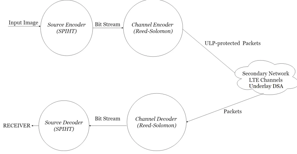
Figure 4.1 shows the proposed end-to-end system setup in the secondary network, where it is operating under the underlay DSA paradigm.

Figure 4.1: End-to-end system setup

indepen-CHAPTER 4. PROPOSED METHODOLOGY

dently designed. Regular JSCC setup is very effective for multimedia transmissions because of its ability to trade off between distortion and compression rate to reduce consumption of bandwidth [20]. This setup is similar to those proposed by Chaoub and Ibn-Elhaj [14], Mohr and Riskin [2], and Chande and Farvardin [18]. However, Chaoub and Ibn-Elhaj’s model operates under the interweave DSA paradigm, where the secondary network is ”opportunistic” in its transmissions. This scheme finds spectrum holes through the estimation of the primary network’s arrival as a Poisson process. The setup in this thesis operates under the underlay DSA paradigm and can transmit at any time and at any frequency band, providing that the interference temperature caused at the primary network is kept at a reasonable level. Mohr and Riskin uses only a single channel while incorporating different channel loss profiles such as uniform, binomial, and exponential distributions [2]. This thesis allows for multi-channel transmissions. Finally Chande and Farvardin utilizes rate-compatible punctured convolutional codes as channel codes so that the transmission is optimized at any transmission rate; whereas this work uses Reed-Solomon codes.

4.2

Implementation Details

4.2.1 Source Encoder - SPIHT

CHAPTER 4. PROPOSED METHODOLOGY

SPIHT encoding and decoding as well as evaluating results.

Figure 4.2: Block diagram of the research tool’s usage in this work

CHAPTER 4. PROPOSED METHODOLOGY

4.2.2 Channel Encoder

The channel encoder is designed in a way to maximize the expected PSNR for the image, taken into account various factors such as the PSNR obtained at different source bit stream truncation cutoff percentages, the number of channels available for transmission, the capacity of such channels, and the number of packets intended to be sent.

a) RS Coding

RS coding is used here as erasure codes to provide the forward error correction (FEC) property to the bit stream, now placed in source packets, and protect it from channel errors. For the codeRS(N, k) containingN packets (or symbols), the entire codeword is in error if there are more thant =bN−k

2 cpacket losses. If the probability of packet

loss is π, for each value of m > t, the probability of the codeword being in error is equivalent to the probability of losing any m packets out of the original N:

Pe(N, m, π) =

N m

πm(1−π)N−m (4.1)

Therefore, the probability of decoding error for code RS(N, k) is the probability of losing t or more packets based on Equation 4.1, and also as described in [21]:

Pe(N, t, π) = N

X

m=t+1

N m

πm(1−π)N−m (4.2)

b) Channel Properties

CHAPTER 4. PROPOSED METHODOLOGY

through the channel. Kwasinski and Shah Mohamadi in [17] were able to implement a cognitive engine that allows the secondary users to transmit autonomously at the largest possible throughput value allowed by the PN. The result of their work is shown in Figure 4.3 where the PN load and the secondary network throughput was calculated under different operating conditions. Out of these results, utilized in this thesis is the curve where the relative throughput change at the PN is less than 2% and seven probe messages are transmitted, because this condition affects the primary network the least (only 2% relative throughput change compared to 5% and 10% in others). For this curve, the values of the PN load and the secondary network throughput formed a linear relationship, allowing the throughput to be estimated based on the PN load at any point in time.

Figure 4.3: Average secondary network throughput under different PN loads [17]

CHAPTER 4. PROPOSED METHODOLOGY

Table 4.1: PN load and secondary network throughput, PN relative throughput change = 2%

Primary Network Load Secondary Network Throughput [Mbps]

0.16 0.1325

0.32 0.1

0.48 0.07

0.64 0.05

Y, the relationship between X and Y can be approximated from Figure 4.3 as

Y =aX+b (4.3)

Where a is calculated to be -0.1734 and b is calculated to be 0.1535, using linear regression for the data points given in Table 4.1. Because X is a random variable,

Y, as a function of X, is also a random variable. As the primary network load, we assumed that X follows an uniform distribution between 0.16 and 0.64, which means its cdf is

FX(x) =

x−0.16

0.48 . (4.4) From equation 4.3 the cdf of Y is calculated as,

FY(y) = 1−FX

y−b a

, a <0. (4.5)

Combining (4.4) and (4.5) the cdf of Y is

FY(y) = 1− y−b

a −0.16

0.48 = 1−y−b−0.16a

0.48a

= −1

0.48ay+z,

CHAPTER 4. PROPOSED METHODOLOGY

and, therefore, the pdf of Y is

fY(y) = FY0 (y)

= −1 0.48a =

1 0.0832.

(4.7)

Y, therefore, is uniformly distributed between 0.1325 and 0.05.

c) LTE

The setup for this research consists of a multichannel CR network, where there are multiple LTE channels. Each channel corresponds to one resource block as part of a LTE frame lasting 10ms in duration. The frame can contain 20 RBs horizontally and up to 50 RBs vertically if the bandwidth is 10Mhz. Figure 4.4 shows an illustration of an FDD frame, where a frame contains 120 RBs (20 horizontal, 6 vertical for 1.4MHz bandwidth) at a duration of 0.5ms each.

Figure 4.4: Illustration of an FDD frame [22]

CHAPTER 4. PROPOSED METHODOLOGY

1s/0.5ms= 2000 RBs. This leads to the number of bits per RB as:

1000000Y[bits/sec]

2000[RB/sec] = 500Y[bits/RB]. (4.8)

As Y takes values between 0.05 and 0.1325, the number of bits per RB is between 25 and 66. For a horizontal segment of the frame with 20 RBs in it, the capacity of a channel, then, is anywhere from 500[bits/f rame] to 1320[bits/f rame]. The more channels that exist, the higher the amount of bits that could be sent over through every channel without exceeding each channel capacity.

d) ULP FEC Allocation Problem Description

The ULP assignment of error-correction bits to packets in the stream needs to maxi-mize the expected quality of the output image, or in other words, the expected PSNR of the output image, denoted as P SN R. Given RS code (N, k) where the probability of symbol error isπ, as well as the total amount of source packets beingS, P SN Ris calculated using the following formula:

P SN R=∆

S

X

i=0

P SN R(Pi)Pi|0(π) (4.9)

where: P SN R(Pi) is the PSNR performance of the source coder after the ith packet

is decoded successfully, and the conditional probability Pi|0(π), introduced in [11] as

CHAPTER 4. PROPOSED METHODOLOGY

first 0 packets are decoded correctly, is defined as

Pi|0(π) ∆ =               

Pe(N,1, π), i= 0,

Pe(N, i+ 1, π)Qi_j=1(1−Pe(N, j, π)), i= 1,2, . . . , S −1,

QS

j=1(1−Pe(N, j, π)), i=S,

(4.10)

where Pe(N, t, π) was defined in (4.2).

Denote the family of error correction-detection channel codes by C ={c1, c2, . . . , cN}

and the Reed-Solomon code rates to be rc(ci), i = 1, . . . , N. This means that a

codeword for the source packet with lengthk bits and protected by codeci has length

k/rc(ci) bits. Now define the probability of packet decoding failure for a given channel

with codeci ∈ C to bePe(ci) (soPe(c0) = 1). With that in mind, the ULP allocation

comes into play to assign a channel code to each source packet before transmission. A code allocation policy φ is created to allocate channel code ci

φ ∈ C to the ith

packet out of the source coder. The policy φ contains a sequence of channel codes

c1_φ, c2_φ, . . . , cN_φ . The normalized transmission rate for such policy (in channel bits per source sample), given that rs is the bits per sample source packet, is therefore

RTπ

∆ = S X i=1 rs

rc(ciφ)

. (4.11)

The optimization problem then is defined as

maxP SN R subject toRTπ ≤R (4.12)

CHAPTER 4. PROPOSED METHODOLOGY

e) Solving the ULP FEC Allocation Problem

For RS code, the family code to pick from is {1/N,2/N, . . . , N/N}. Each source packet out of S in the stream will be assigned a code from this list, and therefore there areNS possible ways to assign FEC bits to the packets. TO find the best ULP FEC allocation, every single combination out of theseNS _{ways is examined, and the}

combination that yields the highest expectedP SN Ris chosen to encode the packets.

From (4.10) it could be seen that the conditional probability Pi|0(π) is constant ifS,

the number of packets, as well asπ, the probability of symbol error, stay the same. If

Pi|0(π) is constant, according to Equation 4.9, the value of the quantity P SN R(Pi)

determines the maximum P SN R for the image.

The calculation of P SN R(Pi) depends on many factors. First, from the channel

statistics, it is possible to find the maximum capacity of a channel to send bits through. Equation (4.8) can be used to find the maximum amount of bits a chan-nel can handle per frame, which is 20 times of the amount the chanchan-nel can handle per resource block. The total amount of bits the channel can handle is simply the sum of its subchannels. For example, if the subchannels have the Y-values equal to

{0.05,0.08,0.1}, then their respective bits per resource block is {25,40,50}, which leads to the capacity per channel being{500,800,1000}and the total amount of bits possible to send equal to 2300. Denote this quantity, the calculated channel capacity, as V. Then the channel encoder can only send V amount of bits through, and since the stream is already SPIHT-encoded, the channel encoder will send the first V bits of the stream as shown in Figure 4.5. Because there are S packets and the codeword length is N, that leaves b V

SNc bits per packet, information or redundancy. A RS

Code (N, k) will select kb V

SNc bits from the stream as data, while leaving the rest

CHAPTER 4. PROPOSED METHODOLOGY

Figure 4.5: Bits selection from the output SPIHT stream

The number of bits theoretically received up to the ith _{packet is calculated, which}

will give the packet loss rate as 1 - (number of bits received) / (bit stream original length). P SN R(Pi) can be found by performing linear interpolation on the PSNR

versus packet loss rate curve.

4.2.3 Rest of System

Assume that the channel loss profile indicates that the transmission success proba-bility for every packet to be 80%. The transmission criteria is that all packets should ideally transmit in one channel only, however each packet can be split up in many parts to transmit at once over multiple channels. Once the packets go through the lossy channels, the channel decoder is notified at the RB level whether the content in the RBs are lost over the channel, and if so, at which location in the frame. These information are useful at determining the faulty RS codes, which have more than the acceptable amount of packet losses, to discard them. If the code containing layer i

is discarded, no more decoding is further needed; the stream has to receive layer i

Chapter 5

Experimental Evaluation

5.1

Experimental Setup

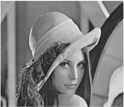
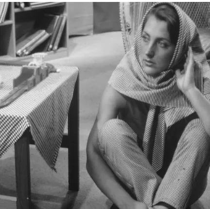
The images used to test the system setup are 512 x 512 bitmap images of Lena, Goldhill and Barbara, as shown in Figures 5.1, 5.2, and 5.3 respectively. For SPIHT encoding, all of the SPIHT properties are selected so that the compression of the stream is the most effective: SPIHT utilizes the 9/7-tap biorthogonal wavelet filter, with 8 filtering levels and 11 bit planes to decode. The compression ratio is set to 8, which is equivalent to the bits per pixel rate being exactly 1.0. Number of packets (S) is set to 5, codeword length (N) for RS coding is set to 14. The primary network load is randomized from 0.16 to 0.64 using (4.7), from which the channel capacity is calculated and become part of the algorithm to solve the ULP FEC allocation problem.

5.1.1 ELP Test

CHAPTER 5. EXPERIMENTAL EVALUATION

Figure 5.1: Original Lena image

CHAPTER 5. EXPERIMENTAL EVALUATION

Figure 5.3: Original Barbara image

assignment is the ELP allocation with maximum P SN R. At this point, all layers should have about the same amount of source packets, and therefore about the same amount of error correction packets. Each of the redesigned combinations, then, will produce a maximumP SN Rvalue and the most optimal code rate assignment, which is then compared to the results obtained through ULP.

5.2

Results and Analysis

5.2.1 SPIHT Encoder

CHAPTER 5. EXPERIMENTAL EVALUATION

original SPIHT work and contained a collection of different bits per pixel (bpp) rate. It could be seen that the performances are very similar in both case for both Lena and Goldhill images; however, the original SPIHT simulation results does not feature PSNR values at 0.2bpp or less. There is a significant dropoff in PSNR at around 95% packet loss rate. Overall, the similarity in terms of results for the SPIHT Encoder ensures that the bit stream is encoded correctly using the given tool.

(a) Packet loss vs. PSNR

(b) BPP vs. PSNR [8]

Figure 5.4: Comparison of SPIHT encoding efficiencies: (a) with the tool (b) original code [8]

Figure 5.5 again demonstrates that the tool performs as expected. The pattern of PSNRs is similar for both images, and both suffer a dropoff in quality near the 95% mark.

5.2.2 Channel Encoder

CHAPTER 5. EXPERIMENTAL EVALUATION

(a) Compression Ratio 8 (b) Compression Ratio 40

Figure 5.5: Comparison of SPIHT encoding efficiencies with the tool (a) compression ratio 8 (b) compression ratio 40

different number of channels of 3, 6, 12, 24 and 48, and two different codeword length of 14 and 15. The varying channel packet loss rates were chosen such that the setup can be tested under varying packet loss conditions, with the most extreme condition being 40% channel packet loss rate. The number of channels were selected such that a varying amount of channel bandwidth was tested with the setup, and that at 48 channels, taking up three horizontal bands of a LTE frame, the channel bandwidth is large enough to accommodate all of the source bit stream. Because the primary network load is random, the secondary network throughput and the channel bandwidths are also random. Therefore, to accurately assess the results of the setup, 20 simulations were conducted, each with a randomized primary network load; the code rate selections as well as the P SN R results were averaged over these 20 runs.

a) Codeword length 14

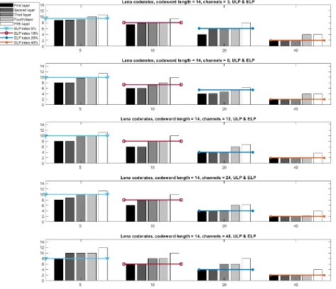
CHAPTER 5. EXPERIMENTAL EVALUATION

loss rate. Then each group has five bars representing the ULP rate selection for each of the five layers. For all groups in the graph, the ULP rate selection indicates the number of information packets included in the codeword of length 14. Each group also contains a horizontal line, indicating the ELP code rate selection.

It could be seen from Figure 5.6 that for all groups in the graph, the ULP rate selection is unequal for all layers: the rate is non-decreasing from the first layer to the last in each group, as is to be expected because higher loss rate will require larger error protection. In other words, the first layer is protected the most and no less than the second layer, the second layer is protected no less than the third layer, and so on. The reason is that as the bit stream from SPIHT encoding is embedded, layers from first to last have decreasing amount of importance, and furthermore, a layer can only be used for decoding if all the previous layers have been received with no errors. As indicated in (4.9), maximizing P SN R is to maximizePi|0(π) when possible, and

maximizing Pi|0(π) generally means increasing the protection for the more important

CHAPTER 5. EXPERIMENTAL EVALUATION

stream, and therefore increasing the channel bandwidth to transmit only helps with transmitting the latter part of the stream, which has very little effect on the decoded image quality because of its lower importance. Both ULP and ELP code rate selection values in all groups, when rounded to the nearest integer, are mostly even due to the effect of padding.

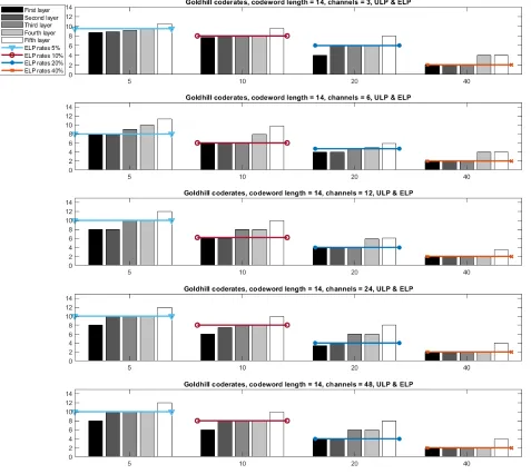
Similar conclusions can also be drawn from Figures 5.7 and 5.8, which show the results of code rate selection for the Goldhill and Barbara images, averaged after 20 simulations, with codeword length 14 and for both ULP and ELP frameworks. For Goldhill, the ELP rate selection for all groups, compared to the ULP rate selection, tends to protect the first two layers less (rather than three for Lena) and the last three layers more (rather than two for Lena). This is possibly a result of the Goldhill image relying on less amount of important packets to decode than Lena, a consequence of different image compositions: one describes a scenery and the other describes a person’s face.

Figure 5.9 shows the P SN R results for Lena, averaged after 20 simulations, with codeword length 14 and using the ULP framework. The benchmark line indicates the PSNR value of the Lena image when transmitted without errors. Each curve represents theP SN Rfor a channel packet loss rate with varying number of channels. TheP SN Rcorresponds directly to the decoded image quality; the higher theP SN R

value, the better the decoded image quality is. For the test images in this thesis, the

P SN Ris considered good, acceptable, or bad based on the values in Table 5.1. Good or benchmark P SN R means that the decoded image quality is excellent; acceptable

P SN R means that despite some distortions, the decoded image is still recognizable; and bad P SN R means that the decoded image is no longer recognizable.

It is clear from the figure that as channel packet loss rate increases, the P SN R

CHAPTER 5. EXPERIMENTAL EVALUATION

Figure 5.6: Lena’s average code rate selection results for ULP and ELP, codeword length 14

rate generally means Pi|0(π) decreases, which from the calculation ofP SN R in (4.9)

CHAPTER 5. EXPERIMENTAL EVALUATION

Figure 5.7: Goldhill’s average code rate selection results for ULP and ELP, codeword length 14

CHAPTER 5. EXPERIMENTAL EVALUATION

Figure 5.8: Barbara’s average code rate selection results for ULP and ELP, codeword length 14

CHAPTER 5. EXPERIMENTAL EVALUATION

Images Benchmark Good Acceptable Bad Lena 39.950 26 - 39.95 20-26 <20 Goldhill 35.873 23 - 35.873 19-23 <19 Barbara 35.820 23 - 35.82 19-23 <19

Table 5.1: P SN R values classification for the test images

Similar conclusions can also be drawn from Figures 5.10 and 5.11, which show the

P SN R results for the Goldhill and Barbara images, averaged after 20 simulations, with codeword length 14 and using the ULP framework.

Figure 5.9: Lena’s average P SN R results for ULP, codeword length 14

CHAPTER 5. EXPERIMENTAL EVALUATION

Figure 5.10: Goldhill’s average P SN R results for ULP, codeword length 14

Figure 5.11: Barbara’s averageP SN R results for ULP, codeword length 14

as manifestations of Figure 5.10 and 5.11.

CHAPTER 5. EXPERIMENTAL EVALUATION

Figure 5.12: Lena’s decoded images using ULP with codeword length 14

Lena with codeword length 14 using the ULP framework, using the P SN R values obtained through the ELP framework as a reference. Each curve represents the

P SN R difference for a channel packet loss rate with varying number of channels, where each point in the curve is calculated in this formula:

P SN R difference =P SN R for ULP−P SN R for ELP (5.1)

CHAPTER 5. EXPERIMENTAL EVALUATION

Figure 5.13: Goldhill’s decoded images using ULP with codeword length 14

Figure 5.6, in which ELP tends to protect more important layers less and less impor-tant layers more than ULP does, resulting in theP SN Rvalue being smaller asPi|0(π)

is smaller for ELP due to the higher code rates chosen at the more important layers. This is also observed in Figures 5.16 and 5.17 for Goldhill and Barbara respectively, which confirms ULP’s superior performance over ELP for codeword length 14.

CHAPTER 5. EXPERIMENTAL EVALUATION

Figure 5.14: Barbara’s decoded images using ULP with codeword length 14

CHAPTER 5. EXPERIMENTAL EVALUATION

Figure 5.15: Lena’s average P SN Rresults for ULP relative to ELP, codeword length 14

Figure 5.16: Goldhill’s averageP SN R results for ULP relative to ELP, codeword length 14

CHAPTER 5. EXPERIMENTAL EVALUATION

Figure 5.17: Barbara’s averageP SN R results for ULP relative to ELP, codeword length 14

padding. Similar conclusions can also be drawn from Figures 5.19 and 5.20, which show the results of code rate selection for the Goldhill and Barbara images, averaged after 20 simulations, with codeword length 15 and for both ULP and ELP frameworks.

Figure 5.21 shows the P SN R results for Lena, averaged after 20 simulations, with codeword length 15 and using the ULP framework. It could be seen from the figure that except for the data points in the 40% channel packet loss rate curve, the difference in performance between codeword length 15 and 14 is small enough that the decoded images would look extremely similar in both cases. This is also observed in Figures 5.23 and 5.22 where the P SN R results for Barbara and Goldhill are shown.

CHAPTER 5. EXPERIMENTAL EVALUATION

Figure 5.18: Lena’s average code rate selection results for ULP and ELP, codeword length 15

anyway), all of the relative values in Figure 5.24 are positive, showing the higher

CHAPTER 5. EXPERIMENTAL EVALUATION

Figure 5.19: Goldhill’s average code rate selection results for ULP and ELP, codeword length 15

CHAPTER 5. EXPERIMENTAL EVALUATION

Figure 5.20: Barbara’s average code rate selection results for ULP and ELP, codeword length 15

value being smaller asPi|0(π) is smaller for ELP due to the higher code rates chosen at

CHAPTER 5. EXPERIMENTAL EVALUATION

Figure 5.21: Lena’s average P SN Rresults for ULP, codeword length 15

Figure 5.22: Goldhill’s average P SN R results for ULP, codeword length 14

CHAPTER 5. EXPERIMENTAL EVALUATION

Figure 5.23: Barbara’s averageP SN R results for ULP, codeword length 15

CHAPTER 5. EXPERIMENTAL EVALUATION

Figure 5.25: Goldhill’s averageP SN R results for ULP relative to ELP, codeword length 15

Chapter 6

Conclusions & Future Work

The ever increasing demands for spectrum access and the growing amount of multi-media communication needs will only increase the usage of CRs in wireless networks for multimedia transmissions as means to dynamically access the radio spectrum while operating with the best possible throughput amount. This work proposed an end-to-end JSCC system setup for transmissions of images over a lossy multichan-nel CR network operating with the underlay DSA paradigm. The system contains a pair of jointly-configured source-channel codecs: the source encoder is in the form of SPIHT, while the channel encoder processes information about the bit stream and the channel characteristic so that it can assign packets the appropriate amount of FEC bits to maximize the expected PSNR of the output image. Theoretical analysis of the code rate selection process is supported by the practical simulations of an image transmission under this system.

ac-CHAPTER 6. CONCLUSIONS & FUTURE WORK

Bibliography

[1] S. Haykin, “Cognitive radio: brain-empowered wireless communications,” IEEE Journal on Selected Areas in Communications, vol. 23, no. 2, pp. 201–220, Feb 2005.

[2] A. E. Mohr, E. A. Riskin, and R. E. Ladner, “Unequal loss protection: graceful degradation of image quality over packet erasure channels through forward error correction,” IEEE Journal on Selected Areas in Communications, vol. 18, no. 6, pp. 819–828, June 2000.

[3] J. Mitola, “Cognitive radio architecture evolution,” Proceedings of the IEEE, vol. 97, no. 4, pp. 626–641, 2009.

[4] M. Song, C. Xin, Y. Zhao, and X. Cheng, “Dynamic spectrum access: from cognitive radio to network radio,”IEEE Wireless Communications, vol. 19, no. 1, pp. 23–29, February 2012.

[5] A. Goldsmith, S. A. Jafar, I. Maric, and S. Srinivasa, “Breaking spectrum grid-lock with cognitive radios: An information theoretic perspective,” proc. IEEE, vol. 97, no. 5, pp. 894–914, 2009.

[6] V. Towhidlou and M. Shikh-Bahaei, “Cross-layer design in cognitive radio standards,” CoRR, vol. abs/1712.05003, 2017. [Online]. Available: http://arxiv.org/abs/1712.05003

[7] N. Malheiros, D. Kliazovich, F. Granelli, E. Madeira, and N. L. da Fonseca, “A cognitive approach for cross-layer performance management,” in 2010 IEEE Global Telecommunications Conference GLOBECOM 2010. IEEE, 2010, pp. 1–5.

[8] A. Said and W. A. Pearlman, “A new, fast, and efficient image codec based on set partitioning in hierarchical trees,” IEEE Transactions on circuits and systems for video technology, vol. 6, no. 3, pp. 243–250, 1996.

[9] M. Akter, M. Reaz, F. Mohd-Yasin, and F. Choong, “A modified-set partition-ing in hierarchical trees algorithm for real-time image compression,” Journal of Communications Technology and Electronics, vol. 53, no. 6, pp. 642–650, 2008. [10] A. Kwasinski, “Joint source-channel coding for delay-constrained iterative

BIBLIOGRAPHY

[11] A. Kwasinski, P. Cosman, and V. Chande, Joint Source-Channel Coding, ser. Wiley - IEEE. Wiley, 2019, (in press). [Online]. Available: https: //books.google.ae/books?id=TSKJMAEACAAJ

[12] H. Ha and C. Yim, “Scalable video transmission over wireless networks based on loss distribution and layer information,”Wireless Personal Communications, vol. 83, no. 3, pp. 2013–2028, 2015.

[13] S. B. Wicker and V. K. Bhargava, Reed-Solomon codes and their applications. John Wiley & Sons, 1999.

[14] A. Chaoub and E. Ibn-Elhaj, “Cross layer design for equal and unequal loss protection frameworks in cognitive radio networks,”Computers & Electrical En-gineering, vol. 39, no. 2, pp. 571–581, 2013.

[15] H. Kushwaha, Y. Xing, R. Chandramouli, and H. Heffes, “Reliable multimedia transmission over cognitive radio networks using fountain codes,”Proceedings of the IEEE, vol. 96, no. 1, pp. 155–165, 2007.

[16] A. Chaoub, E. I. Elhaj, and J. El Abbadi, “Multimedia traffic transmission over cognitive radio networks using multiple description coding,” in International conference on advances in computing and communications. Springer, 2011, pp. 529–543.

[17] F. S. Mohammadi and A. Kwasinski, “Neural network cognitive engine for au-tonomous and distributed underlay dynamic spectrum access,” arXiv preprint arXiv:1806.11038, 2018.

[18] V. Chande and N. Farvardin, “Joint source-channel coding for progressive trans-mission of embedded source coders,” in Proceedings DCC’99 Data Compression Conference. IEEE, 1999, pp. 52–61.

[19] A. Kwasinski and W. Wang, “Cooperative learning for reduced complexity cross-layer cognitive radio,” in Personal Indoor and Mobile Radio Communications (PIMRC), 2011 IEEE 22nd International Symposium on. IEEE, 2011, pp. 374– 378.

[20] M. F. Sabir, H. R. Sheikh, R. W. Heath, and A. C. Bovik, “A joint source-channel distortion model for jpeg compressed images,” in2004 International Conference on Image Processing, 2004. ICIP’04., vol. 5. IEEE, 2004, pp. 3249–3252. [21] D. Divsalar and J. Yuen, “Performance of concatenated reed-solomon/viterbi

channel coding,” The Telecommunications and Data Acquisition Progress Jour-nal, pp. 81–94, 1982.