Deep Joint Source-Channel Coding for
Wireless Image Transmission
Eirina Bourtsoulatze, David Burth Kurka and Deniz G¨
und¨
uz
Abstract—We propose a joint source and channel coding (JSCC) technique for wireless image transmis-sion that does not rely on explicit codes for either compression or error correction; instead, it directly maps the image pixel values to the complex-valued channel input symbols. We parameterize the encoder and decoder functions by two convolutional neural networks (CNNs), which are trained jointly, and can
be considered as an autoencoder with a non-trainable
layer in the middle that represents the noisy commu-nication channel. Our results show that the proposed deep JSCC scheme outperforms digital transmission concatenating JPEG or JPEG2000 compression with a capacity achieving channel code at low signal-to-noise ratio (SNR) and channel bandwidth values in the presence of additive white Gaussian noise (AWGN). More strikingly, deep JSCC does not suffer from the “cliff effect”, and it provides a graceful performance degradation as the channel SNR varies with respect to the SNR value assumed during training. In the case of a slow Rayleigh fading channel, deep JSCC learns noise resilient coded representations and significantly outperforms separation-based digital communication at all SNR and channel bandwidth values.
Index Terms—Joint source-channel coding, deep neural networks, image communications.
I. Introduction
Modern communication systems employ a two step encoding process for the transmission of image/video data
(see Fig. 1a for an illustration): (i)the image/video data
is first compressed with a source coding algorithm in order to get rid of the inherent redundancy, and to reduce
the amount of transferred information; and (ii) the
com-pressed bitstream is first encoded with an error correcting code, which enables resilient transmission against errors,
and then modulated. Shannon’sseparation theoremproves
that this two-step source and channel coding approach is optimal theoretically in the asymptotic limit of infinitely long source and channel blocks [1]. While in practical
E. Bourtsoulatze is with the Communications and Information Systems Group, Department of Electronic and Electrical Engineer-ing, University College London, London, UK. D. Burth Kurka and D. G¨und¨uz are with the Information Processing and Communications Laboratory, Department of Electrical and Electronic Engineering, Imperial College London, London, UK.
E-mails:[email protected],[email protected], [email protected]
This work has been funded by the European Union’s Horizon 2020 research and innovation programme under the Marie Sk lodowska-Curie fellowship (grant agreement No. 750254) and by the European Research Council (ERC) through the Starting Grant BEACON (grant agreement No. 725731).
applications joint source and channel coding (JSCC) is known to outperform the separate approach [2], sepa-rate architecture is attractive for practical communica-tion systems thanks to the modularity it provides. More-over, highly efficient compression algorithms (e.g. JPEG, JPEG2000, WebP [3]) and near-optimal channel codes (e.g. LDPC, Turbo codes) are employed in practice to approach the theoretical limits. However, many emerging applications from the Internet-of-things to autonomous driving and to tactile Internet require transmission of im-age/video data under extreme latency, bandwidth and/or energy constraints, which preclude computationally de-manding long-blocklength source and channel coding tech-niques.
We propose a JSCC technique for wireless image trans-mission that directly maps the image pixel values to the complex-valued channel input symbols. Inspired by the success of unsupervised deep learning (DL) methods, in particular, the autoencoder architectures [4], [5], we design an end-to-end communication system, where the encoding and decoding functions are parameterized by two convolutional neural networks (CNNs) and the communi-cation channel is incorporated in the neural network (NN)
architecture as a non-trainable layer; hence, the namedeep
JSCC. Two channel models, the additive white Gaussian
noise (AWGN) channel and the slow Rayleigh fading chan-nel, are considered in this work due to their widespread adoption in representing realistic channel conditions. The proposed solution is readily extendable to other channel models, as long as they can be represented as a non-trainable NN layer with a differentiable transfer function. DL-based methods, and, particularly, autoencoders, have recently shown remarkable results in image com-pression, achieving or even surpassing the performance of
state-of-the-art lossy compression algorithms. Ball´eet al.
[6] propose an end-to-end optimized image compression method, consisting of a nonlinear analysis transformation, a uniform quantizer, and a nonlinear synthesis trans-formation. Their method exhibits better rate-distortion performance than JPEG and JPEG2000 in most images, while the visual quality, as captured by the MS-SSIM metric, improves for all test images and over all bitrate values. A compressive autoencoder is used in [7], where the authors propose to use a proxy of the quantization step only in the backward propagation, while keeping the rounding in the forward step. The authors of [8] com-plement the autoencoder based compression architecture with adversarial loss to achieve realistic reconstructions
a convolutional autoencoder based lossy image compres-sion architecture, which achieves on average a 13.5% rate saving versus JPEG2000 on the Kodak image dataset. The advantage of DL-based methods for lossy compres-sion versus conventional comprescompres-sion algorithms lies in their ability to extract complex features from the train-ing data thanks to their deep architecture, and the fact that their model parameters can be trained efficiently on large datasets through backpropagation. While common compression algorithms, such as JPEG, apply the same processing pipeline to all types of images (e.g., DCT trans-form, quantization and entropy coding in JPEG), the DL-based image compression algorithms learn the statistical characteristics from a large training dataset, and optimize the compression algorithm accordingly, without explicitly specifying a transform or a code.
At the same time, the potential of DL has also been capitalized by researchers to design novel and efficient coding and modulation techniques in communications. In particular, the similarities between the autoencoder architecture and the digital communication systems have motivated significant research efforts in the direction of modelling end-to-end communication systems using the autoencoder architecture [10], [11]. Some examples of such designs include decoder design for existing channel codes [12], [13], blind channel equalization [14], learning physical layer signal representation for SISO [11] and MIMO [15] systems, OFDM systems [16], [17], JSCC of text messages [18] and JSCC for MNIST images for analog storage [19]. In this work, we leverage the recent success of DL methods in image compression and communication system design to propose a novel JSCC algorithm for image trans-mission over wireless communication channels. We con-sider both time-invariant and fading AWGN channels, and compare the performance of our algorithm to the state-of-the-art compression algorithms (JPEG and JPEG2000, in particular) combined with capacity-achieving channel codes. We show through experiments that our solution achieves superior performance in low signal-to-noise ratio (SNR) regimes and for limited channel bandwidth, over a time-invariant AWGN channel, even though the separation scheme is assumed to be operating at the channel capacity despite the short blocklengths. While we have mainly focused on the peak signal-to-noise ratio (PSNR) as the performance measure, we show that the deep JSCC can provide even better results when measured in terms of the structural similarity index (SSIM), which better captures the perceived visual quality of the reconstructed images. More interestingly, we demonstrate that our approach is resilient to variations in channel conditions, and does not suffer from abrupt quality degradations, known as the “cliff effect” in digital communication systems: deep JSCC algorithm exhibits graceful performance degradation when the channel conditions deteriorate. This latter property is particularly attractive when broadcasting the same image to multiple receivers with different channel qualities, or when transmitting to a single receiver over an unknown fading channel. Indeed, we show that the proposed deep
JSCC scheme achieves a remarkable performance over a slow Rayleigh fading channel by learning coded represen-tations robust to channel quality fluctuations and outper-forms a separation-based digital transmission scheme even at high SNR and large channel bandwidth scenarios.
This is the first time an end-to-end joint source-channel coding architecture is trained for wireless transmission of high-resolution images over AWGN and fading channels. This architecture allows training for other performance measures or other source signals (e.g., video) as well. Moreover, while the training of the deep JSCC algo-rithm can be fairly time consuming, once the network is trained, the encoding and decoding tasks become ex-tremely fast, compared to applying advanced image com-pression/decompression algorithms followed by capacity-approaching channel coding and decoding. We believe this may be key to enabling many low-latency applications that require the transmission of high data rate content at the wireless edge, such as image/video sensor data from autonomous cars or drones, or emerging AR/VR applications. We also emphasize that the employed neural network architecture is quite efficient consisting of fully convolutional layers. With the rapid advances in hardware accelerators specially optimized for CNNs [20], [21], we believe the deep JSCC can very soon be deployed directly on mobile wireless devices.
The rest of the paper is organized as follows. In Sec-tion II, we introduce the system model, provide some background on the conventional wireless image trans-mission systems and their limitations, and motivate our novel approach. We introduce the proposed deep JSCC architecture in Section III. Section IV is dedicated to the evaluation of the performance of the proposed deep JSCC scheme, and its comparison with the conventional separate JSCC schemes over both static and fading AWGN channels. Finally, the paper is concluded in Section V.
II. Background and Problem Formulation We consider image transmission over a point-to-point wireless communication channel. The transmitter maps
the input image x ∈ Rn to a vector of complex-valued
channel input symbols z ∈ Ck. Following the JSCC
literature, we will call the image dimensionnas thesource
bandwidth, and the channel dimension k as the channel bandwidth. We typically have k < n, which is called band-width compression. We will refer to the ratiok/nas band-width compression ratio. Due to practical considerations in real-world communication systems, e.g., limited energy,
interference, etc., the output of the transmitter may be
required to satisfy a certain power constraint, such as peak and/or average power constraints. The output signal
z is then transmitted over the channel, which degrades
the signal quality due to noise, fading, interference or other channel impairments. The corrupted output of the
communication channel ˆz ∈ Ck is fed to the receiver,
which produces an approximate reconstruction ˆx ∈ Rn
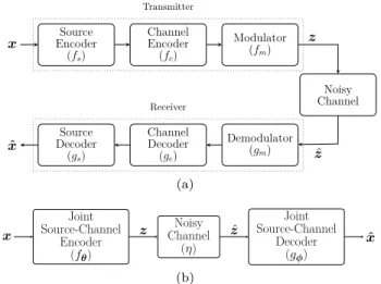
x EncoderSource (fs) Channel Encoder (fc) Modulator (fm) Noisy Channel Demodulator (gm) Channel Decoder (gc) Source Decoder (gs) ˆ x Transmitter Receiver z ˆ z (a) x Joint Source-Channel Encoder (fθ) Noisy Channel (η) Joint Source-Channel Decoder (gφ) ˆ x z zˆ (b)
Fig. 1. Block diagram of the point-to-point image transmission system: (a) components of the conventional processing pipeline and (b) components of the proposed deep JSCC algorithm.
In conventional image transmission systems, depicted in Fig. 1a, the transmitter performs three consecutive
independent steps in order to generate the signalz
trans-mitted over the channel. First, the source redundancies
are removed with a source encoder fs, which is typically
one of the commonly used compression methods (e.g.,
JPEG/JPEG2000, WebP). A channel codefc(e.g., LDPC,
Turbo code) is then applied to the compressed bitstream in order to protect it against the impairments introduced by the communication channel. Finally, the coded bitstream
is modulated with a modulation scheme fm (e.g., BPSK,
16-QAM) which maps the bits to complex-valued samples. The modulated symbols are then carried by the I and Q digital signal components over the communication link (the latter two components are often combined into a single coded-modulation step [22]).
The decoder inverts these operations in the reverse order. It first demodulates and maps the complex-valued channel output samples to a sequence of bits (or, log
likelihood ratios) with a demodulation scheme gm that
matches the modulator fm. It then decodes the channel
code with a channel decoding algorithm gc, and finally
provides an approximate reconstruction of the transmitted image from the (possibly corrupted) compressed bitstream
by applying the appropriate decompression algorithm,gs.
Though the above encoding process is highly optimized and widely adopted in image transmission systems [23], its performance may suffer severely when the channel conditions differ from those for which the system has been optimized. Although the source and channel codes can be designed separately, their rates are chosen jointly targeting a specific channel quality, i.e., assuming that a capacity achieving channel code can be employed, the compression rate is chosen to produce exactly the amount of data that can be reliably transmitted over the channel. However, when the experienced channel condition is worse than the one for which the code rates are chosen, the error prob-ability increases rapidly, and the receiver cannot receive
the correct channel codeword with a high probability. This leads to a failure in source decoder as well, resulting in a significant reduction in the reconstruction quality.
Similarly, the separate design cannot benefit from im-proved channel conditions either; that is, once the source and channel coding rates are fixed, no matter how good the channel is, the reconstruction quality remains the same as long as the channel capacity is above the target rate. These two characteristics are known as the “cliff effect”. Various joint source-channel coding schemes have been proposed in the literature to overcome the “cliff effect” [24], [25], and to obtain graceful degradation of the signal quality with channel SNR, which typically combine multi-layer digital codes with multi-layer compression for unequal error protection.
In this paper we take a radically different approach, and leverage the properties of uncoded transmission [26]–[28] by directly mapping the real pixel values to the complex-valued samples transmitted over the communication chan-nel. Our goal is to design a JSCC scheme that bypasses the transformation of the pixel values to a sequence of bits, which are then mapped again to complex-valued channel inputs; and instead, directly maps the pixel values to channel inputs as in [27], [28].
III. DL-based JSCC
Our design is inspired by the recent successful applica-tion of deep NNs (DNNs), and autoencoders, in particular, to the problem of source compression [6], [7], [9], [29], as well as by the first promising results in the design of end-to-end communication systems using autoencoder architectures [10], [11].
The block diagram of the proposed JSCC scheme is
shown in Fig. 1b. The encoder maps the n-dimensional
input image x to a k-length vector of complex-valued
channel input samplesz, which satisfies the average power
constraint k1E[z∗z] ≤ P, by means of a deterministic
encoding function fθ : Rn → Ck. The encoder function
fθ is parameterized using a CNN with parameters θ.
The encoder CNN comprises a series of convolutional layers followed by parametric ReLU (PReLU) activation functions [30] and a normalization layer. The convolutional layers extract the image features, which are combined to form the channel input samples, while the nonlinear activation functions allow to learn a non-linear mapping from the source signal space to the coded signal space.
The output ˜z ∈Ck of the last convolutional layer of the
encoder is normalized according to:
z= √
kP√z˜ ˜
z∗z˜ (1)
where ˜z∗ is the conjugate transpose of ˜z, such that
the channel input z satisfies the average transmit power
constraintP.
Following the encoding operation, the joint
source-channel coded sequencez is sent over the communication
channel by directly transmitting the real and imaginary parts of the channel input samples over the I and Q
components of the digital signal. The channel introduces random corruption to the transmitted symbols, denoted by η :Ck →
Ck. To be able to optimize the communication
system in Fig. 1b in an end-to-end manner, the communi-cation channel must be incorporated into the overall NN architecture. We model the communication channel as a series of non-trainable layers, which are represented by
the transfer function ˆz = η(z). We consider two widely
used channel models:(i)the AWGN channel, and(ii)the
slow fading channel. The transfer function of the Gaussian channel isηn(z) =z+n, where the vectorn∈Ckconsists of independent identically distributed (i.i.d.) samples from a circularly symmetric complex Gaussian distribution, i.e.,
n∼ CN(0, σ2I
k), whereσ2 is the average noise power. In
the case of slow fading channel, we adopt the commonly used Rayleigh slow fading model. The multiplicative effect of the channel gain on the transmitted signal is captured
by the channel transfer function ηh(z) = hz, where
h ∼ CN(0, Hc) is a complex normal random variable.
The joint effect of channel fading and Gaussian noise can be modelled by the composition of the transfer functions ηh and ηn: η(z) = ηn(ηh(z)) = hz +n. Other channel
models can be incorporated into the end-to-end system in a similar manner with the only requirement that the channel transfer function is differentiable in order to allow gradient computation and error back propagation.
The receiver comprises a joint source-channel decoder. The decoder maps the corrupted complex-valued signal
ˆ
z = η(z) ∈ Ck to an estimation of the original input
ˆ
x ∈ Rn using a decoding function g
φ : Ck → Rn. Similarly to the encoding function, the decoding function is parameterized by the decoder CNN with parameter
set φ. The NN decoder inverts the operations performed
by the encoder by passing the received (and possibly
corrupted) coded signal ˆz through a series of transpose
convolutional layers (with non linear activation functions)
in order to map the image features to an estimate ˆxof the
originally transmitted image.
The encoding and decoding functions are designed jointly to minimize the average distortion between the
original input image xand its reconstruction ˆxproduced
by the decoder:
(θ∗,φ∗) = arg min
θ,φ E
p(x,ˆx)[d(x,xˆ)], (2)
where d(x,xˆ) is a given distortion measure, and p(x,xˆ) is the joint probability distribution of the original and reconstructed images. Since the true distribution of the
input data p(x) is often unknown, an analytical form of
the expected distortion in Eq. (2) is also unknown. We, therefore, estimate the expected distortion by sampling from an available dataset.
IV. Evaluation
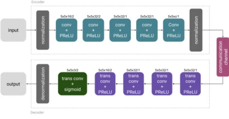
To demonstrate the potential of our proposed deep JSCC scheme, we use the NN architecture depicted in Fig. 2. At the encoder, the normalization layer is followed by five convolutional layers. Since the statistics of the input
Fig. 2. Encoder and decoder NN architectures used in the imple-mentation of the proposed deep JSCC scheme.
data are generally not known at the decoder, the input images are normalized by the maximum pixel value 255,
producing pixel values in the [0,1] range. The notation
F×F×K/Sdenotes a convolutional layer withK filters
of spatial extent (or size) F and stride S. The values of
the hyperparametersF, K andS used in our experiments
are given in Fig. 2. PReLU activation function is applied to the output of all convolutional layers. The output of
the last convolutional layer, which consists of 2k units, is
followed by another normalization layer which enforces the average power constraint specified in Eq. (1). The output
of the normalization layer is combined into k
complex-valued channel input samples and forms the encoded signal representation, which is transmitted over the channel.
The decoder inverts the operations performed by the
encoder. The real and imaginary parts of thek
complex-valued noisy channel output samples are combined into
2k values which are fed into the transpose convolutional
layers. The latter progressively transform the corrupted image features into an estimation of the original input image, while upsampling it to the correct resolution. The hyperparameters of the decoder layers mirror the corresponding values of the encoder layers (Fig. 2). The output of all transpose convolutional layers of the decoder except for the last one are passed through a PReLU activation function, while a sigmoid nonlinearity is applied to the output of the last transpose convolutional layer
in order to produce values in the [0,1] range. Finally, a
denormalization layer multiplies the output values by 255
in order to generate pixel values within the [0,255] range.
The above architecture is implemented in Tensorflow [31]. We use the Adam optimization framework [32], which is a form of stochastic gradient descent. Our loss function is the average mean squared error (MSE) between the
original input image x and the reconstruction ˆx at the
output of the decoder, defined as:
L= 1 N N X i=1 d(xi,xˆi), (3)
whered(x,xˆ) =n1||x−xˆ||2is the mean squared-error
various bandwidth compression ratios k/n, we vary the
number of filters K in the last convolutional layer of
the encoder. Since our architecture is fully convolutional, it can be trained and deployed on input images of any resolution.
The performance of the deep JSCC algorithm, as well as of all benchmark schemes is quantified in terms of PSNR. The PSNR metric measures the ratio between the maximum possible power of the signal and the power of the noise that corrupts the signal. The PSNR is defined as follows:
PSNR = 10 log10
MAX2
MSE (dB). (4)
where MSE =d(x,xˆ) is the mean squared-error between
the reference imagexand the reconstructed image ˆx, and
MAX is the maximum possible value of the image pixels. All our experiments are conducted on 24-bit depth RGB images (8 bits per pixel per colour channel), thus MAX =
28−1 = 255.
The channel SNR is defined as:
SNR = 10 log10
P
σ2 (dB), (5)
and represents the ratio of the average power of the coded signal (channel input signal) to the average noise power.
Recall that P is the average power of the channel input
signal after applying the power normalization layer at the encoder of the proposed JSCC scheme. For benchmark
schemes that use explicit signal modulation, P is the
average power of the symbols in the constellation. Without
loss of generality, we set the average signal power toP = 1
for all experiments.
A. Evaluation on CIFAR-10 dataset
We start by evaluating our deep JSCC scheme on the CIFAR-10 image dataset. The training data consists of
50000 32×32 training images [33] combined with
ran-dom realizations of the channel under consideration. The performance of the proposed JSCC scheme is tested on 10000 test images from the CIFAR-10 dataset, which are distinct from the images used for training. We initially set the learning rate to 10−3and reduce it after 500k iterations
to 10−4. We use a mini-batch size of 64 samples and train
our models until the performance on the test set does not improve further. However, we would like to emphasize that we do not use the test set images to optimize the network hyperparameteres. During performance evalua-tion we transmit each image 10 times in order to mitigate the effect of randomness introduced by the communication channel.
We first investigate the performance of our proposed deep JSCC algorithm in the AWGN setting, i.e., the
channel transfer function is η=ηn. We vary the SNR by
varying the noise variance σ2 and compare the proposed
deep JSCC algorithm with an upper bound on any digital transmission scheme, which employs JPEG or JPEG2000 for source compression. The computation of the upper
bound is based on the Shannon’s separation theorem, which states that the necessary and sufficient condition for reliable communication over a discrete memoryless channel
with channel capacityC is
nR≤kC. (6)
The above expression defines the maximum rate
Rmax=
k
nC (7)
for a channel with capacityC at which the source can be
compressed and transmitted with arbitrarily small proba-bility of error. Thus, to compute the upper bound, we first compute the maximum number of bits per source sample
Rmax using Eq. (7), whereC= log2(1 + SNR) for a
com-plex AWGN channel. This is the maximum rate for source compression that is guaranteed reliable transmission over the channel. Since JPEG and JPEG2000 cannot compress the image data at an arbitrarily low bitrate, we also
compute the minimum bitrate value Rmin beyond which
compression results in complete loss of information and the original image cannot be reconstructed. If, for a given set
of values ofn,kandC, the minimum rateRminexceeds the
maximum allowable rateRmax, we assume that the image
cannot be reliably transmitted and each color channel is reconstructed to the mean value of all the pixels for that
channel. WhenRmin< Rmax, we compress the images at
the largest rateRthat satisfiesR≤Rmax (since, again, it
is not always possible to achieve an arbitrary target bitrate
Rmax with JPEG or JPEG2000 compression software),
and measure the distortion between the reference image and the compressed one, assuming that the compressed bitstream can be transmitted without errors.
We would like to note that we do not use any explicit practical channel coding and modulation scheme in the computation of the bound. Compressing the source at rate
Rmax and assuming error-free transmission at this rate,
implicitly suggests that one would need to use a capacity-achieving combination of channel code and modulation scheme to achieve reliable transmission. Thus, the perfor-mance of any digital transmission scheme that employs an actual channel coding scheme and modulation along with JPEG/JPEG2000 compression will be inferior to this upper bound.
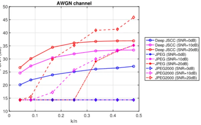
Fig. 3 illustrates the performance of the proposed deep JSCC algorithm with respect to the bandwidth
compression ratio, k/n, in different SNR regimes. This
performance is compared against the upper bound on the performance of any digital scheme that employs JPEG/JPEG2000 for compression. We note that the threshold behavior of the upper bound in the figure is not due to the “cliff effect”. The initial flat part of these curves is due to the fact that JPEG and JPEG2000 completely break down in this region, i.e., the maximum transmission
rateRmaxis below the minimum number of bits per pixel,
Rmin, required to compress the images at the worst quality
0 0.1 0.2 0.3 0.4 0.5 k/n 10 15 20 25 30 35 40 45 50 PSNR (dB) AWGN channel Deep JSCC (SNR=0dB) Deep JSCC (SNR=10dB) Deep JSCC (SNR=20dB) JPEG (SNR=0dB) JPEG (SNR=10dB) JPEG (SNR=20dB) JPEG2000 (SNR=0dB) JPEG2000 (SNR=10dB) JPEG2000 (SNR=20dB)
Fig. 3. Performance of the deep JSCC algorithm on CIFAR-10 test images over an AWGN channel with respect to the compression ratio, k/n, for different SNR values. For each case, the same SNR value is used in training and evaluation.
We observe that, in very bad channel conditions (e.g., for SNR=0dB), the digital schemes deploying JPEG or JPEG2000 would break down, while with the proposed deep JSCC scheme transmission is possible with reason-ably good performance. At medium and high SNRs and for limited channel bandwidth, i.e., for k/n∈ [0.04,0.2], the performance of the proposed deep JSCC scheme is considerably above the one that can be achieved by JPEG and JPEG2000 even assuming that reliable transmission
at channel capacity is possible1. Even when the channel
bandwidth becomes less constrained, i.e., for k/n > 0.3,
the performance of the deep JSCC scheme remains com-petitive with its JPEG/JPEG2000 counterparts. The sat-uration of the proposed deep JSCC scheme in the large channel bandwidth regime is possibly due to the limited capability of the particular autoencoder architecture em-ployed, which may be improved, for example, by employing a different activation function than PReLU as in [6], or through incremental training as in [7].
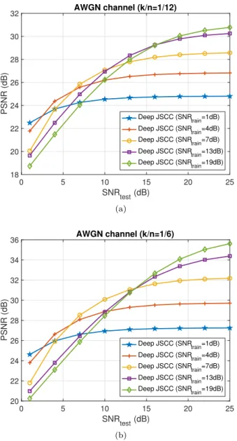
We next study the robustness of the proposed deep JSCC scheme to variations in channel conditions. Figs. 4a and 4b illustrate the average PSNR of the reconstructed images versus the SNR of the AWGN channel for two
different values of bandwidth compression ratio,k/n. Each
curve in Figs. 4a and 4b is generated by training our end-to-end system for a specific channel SNR value,
de-noted as SNRtrain, and then evaluating the performance
of the learned encoder/decoder parameters on the test
images for varying SNR values, denoted as SNRtest. In
other words, each curve represents the performance of the proposed JSCC scheme optimized for channel SNR equal
to SNRtrain, and deployed in different channel conditions
with SNR equal to SNRtest. These results provide an
in-sight into the performance of the proposed algorithm when
1While near capacity-achieving channel codes exist for the AWGN channel, these typically require very large blocklengths. It is known that the achievable rates guaranteeing a low block error probability for the blocklengths considered here are below the capacity [34] for the entire range of compression ratio values. Therefore, the upper bounds in Fig. 3 are typically not achievable.
the channel conditions are different from those for which the end-to-end system is optimized and demonstrate the robustness of the proposed JSCC to variations in channel
quality. We can observe that for SNRtest < SNRtrain,
i.e., when the channel conditions are worse than those for which the encoder/decoder have been optimized, our deep JSCC algorithm does not suffer from the “cliff effect” observed in digital systems. Unlike digital systems, where the quality of the decoded signal drops sharply when
SNRtest drops below a critical threshold value, the deep
JSCC scheme is more robust to channel quality fluctu-ations and exhibits a gradual performance degradation as the channel deteriorates. Such behavior is akin to the performance of an analog scheme [24], [26], [28], and is attributed to the capability of the autoencoder to map similar images/features to nearby points in the channel
input signal space; thus, with decreasing SNRtest the
decoder can still obtain a reconstruction of the original image.
On the other hand, when SNRtest increases above
SNRtrain, we observe initially a gradual improvement in
the quality of the reconstructed images before the
per-formance finally saturates as SNRtest increases beyond
a certain value. The performance in the saturation re-gion is driven solely by the amount of compression im-plicitly decided during the training phase for the
tar-get value SNRtrain. It is worth noting that performance
saturation does not occur at SNRtest = SNRtrain as
in digital image/video transmission systems [27], but at SNRtest > SNRtrain. This behavior indicates that the
proposed JSCC scheme determines an implicit trade-off between the amount of error protection and compression, which does not necessarily target an error-free
transmis-sion when the system operates at SNRtest = SNRtrain. We
also note that when the encoder/decoder are optimized
for very high SNRtrain, and SNRtest > SNRtrain, the
system boils down to an ordinary autoencoder, and its performance is solely limited by the degree-of-freedom
imposed by the bandwidth compression ratiok/n, i.e., the
dimension of the bottleneck layer of the autoencoder. Next we study the performance of our deep JSCC scheme under the assumption of a slow Rayleigh fading channel with AWGN. In this case, the channel transfer
function is η(z) = hz +n, where h ∼ CN(0, Hc) and
n∼ CN(0, σ2I
k). In this experiment, we do not assume
channel state information either at the receiver or the transmitter, or consider the transmission of pilot signals.
As we assume slow fading, the channel gain h is
ran-domly sampled from the complex Gaussian distribution
CN(0, Hc) for each transmitted image and remains
con-stant during the transmission of the entire image, and changes independently to another state for the next image.
We set Hc= 1 and vary the noise varianceσ2 to emulate
varying average channel SNR.
In Fig. 5, we plot the performance of the proposed deep JSCC algorithm over a slow Rayleigh fading channel as
a function of the bandwidth compression ratio, k/n, for
0 5 10 15 20 25 SNRtest (dB) 18 20 22 24 26 28 30 32 PSNR (dB) AWGN channel (k/n=1/12) Deep JSCC (SNRtrain=1dB) Deep JSCC (SNR train=4dB) Deep JSCC (SNRtrain=7dB) Deep JSCC (SNRtrain=13dB) Deep JSCC (SNR train=19dB) (a) 0 5 10 15 20 25 SNRtest (dB) 20 22 24 26 28 30 32 34 36 PSNR (dB) AWGN channel (k/n=1/6) Deep JSCC (SNR train=1dB) Deep JSCC (SNRtrain=4dB) Deep JSCC (SNRtrain=7dB) Deep JSCC (SNRtrain=13dB) Deep JSCC (SNRtrain=19dB) (b)
Fig. 4. Performance of the deep JSCC algorithm on CIFAR-10 test images with respect to the channel SNR over an AWGN channel for bandwidth compression ratios (a)k/n= 1/12 and (b)k/n= 1/6. Each curve is obtained by training the encoder/decoder network for a particular channel SNR value.
of channel state information, the capacity of this channel in the Shannon sense is zero, since no positive rate can be guaranteed reliable transmission at all channel conditions; that is, for any positive transmission rate, the channel capacity will be below the transmission rate with a non-zero probability. Therefore, we calculate an upper bound on any digital transmission scheme designed for the aver-age SNR value. i.e., for SNR = 10 log10E[h2]P
σ2 , which uses
JPEG/JPEG2000 for compression. Similarly to the case of the AWGN channel, we assume that the source image is compressed with JPEG/JPEG2000 at rate that is equal to the capacity of the complex AWGN channel at the average SNR value. That is, we calculate the maximum number of bits that can be transmitted reliably using Eq. (7), where the channel capacity is calculated for the average SNR value. If the channel capacity is below this value due
0 0.2 0.4 0.6 0.8 1 k/n 12 14 16 18 20 22 24 26 28 30 32 PSNR (dB)
Slow Rayleigh fading channel
Deep JSCC (SNR=0dB) Deep JSCC (SNR=10dB) Deep JSCC (SNR=20dB) JPEG (SNR=0dB) JPEG (SNR=10dB) JPEG (SNR=20dB) JPEG2000 (SNR=0dB) JPEG2000 (SNR=10dB) JPEG2000 (SNR=20dB)
Fig. 5. Performance of the deep JSCC algorithm on CIFAR-10 test images over a slow Rayleigh fading channel with respect to the bandwidth compression ratio,k/n, for different SNR values. For each case, the same target SNR value is used in training and evaluation.
to fading, an outage occurs, and the mean pixel values are used for reconstruction, i.e., maximum distortion is reached. If the channel capacity is above the transmission rate, the transmitted codeword can be decoded reliably. We observe that deep JSCC beats the upper bound on the digital transmission schemes at all SNR and bandwidth compression values. This result emphasizes the benefits of the proposed deep JSCC technique when communicating over a time-varying channel, or multicasting to multiple receivers with varying channel states.
We illustrate the robustness of the proposed deep JSCC scheme to variations of the average channel SNR in a slow Rayleigh fading channel in Figs. 6a and 6b. We observe that, while the performance of the deep JSCC scheme drops compared to the static AWGN channel, the quality of the reconstructed images is still reasonable, despite the lack of channel state information. This suggests that the network learns to estimate the channel state, and adapts the decoder accordingly; that is, the proposed deep JSCC scheme combines not only source coding, channel coding, and modulation, but also channel estimation, into one single component, whose parameters are learned through training.
B. Evaluation on the Kodak dataset
We also evaluate the proposed deep JSCC scheme on higher resolution images. To this end, we train our NN architecture on the Imagenet dataset [35] which consists
of 1.2 million images. The images are randomly cropped to
patches of size 128×128 and fed into the network in
mini-batches of 32 samples. We set the learning rate to 10−4
and train the models until convergence. The evaluation
is performed on the Kodak image dataset2 consisting of
24 768×512 images. During evaluation, each image is
transmitted 100 times, so that the performance can be averaged over multiple realizations of the random channel. We first investigate the performance of the proposed deep JSCC algorithm over an AWGN channel by varying
0 5 10 15 20 25 SNRtest (dB) 18 20 22 24 26 28 30 PSNR (dB)
Slow Rayleigh fading channel (k/n=1/6)
Deep JSCC (SNRtrain=1dB) Deep JSCC (SNR train=4dB) Deep JSCC (SNRtrain=7dB) Deep JSCC (SNRtrain=13dB) Deep JSCC (SNR train=19dB) (a) 0 5 10 15 20 25 SNRtest (dB) 18 20 22 24 26 28 30 32 PSNR (dB)
Slow Rayleigh fading channel (k/n=1/3)
Deep JSCC (SNR train=1dB) Deep JSCC (SNRtrain=4dB) Deep JSCC (SNRtrain=7dB) Deep JSCC (SNRtrain=13dB) Deep JSCC (SNRtrain=19dB) (b)
Fig. 6. Performance of the deep JSCC algorithm on CIFAR-10 test images with respect to the average channel SNR over an AWGN slow Rayleigh fading channel for bandwidth compression ratios (a) k/n = 1/6 and (b)k/n= 1/3. Each curve is obtained by training the encoder/decoder network for a particular channel SNR value.
the noise powerσ2. The performance of the proposed deep
JSCC algorithm is compared against digital transmission schemes that use JPEG/JPEG2000 for image compres-sion followed by practical channel coding and modulation
schemes. We use all possible combinations of (4096,8192),
(4096,6144), and (2048,6144) LDPC codes (which
corre-spond to 1/2, 2/3 and 1/3 rate codes) with BPSK, 4-QAM,
16-QAM and 64-QAM digital modulation schemes. For the sake of legibility, we only present the best performing digital transmission schemes and omit those that perform similarly, or whose performance in terms of PSNR is below 15dB.
Figs. 7 and 8 show the performance of the proposed deep JSCC scheme and the digital transmission schemes in an AWGN channel as a function of the test SNR for
bandwidth compression ratiosk/n= 1/12 andk/n= 1/6,
-2 1 4 7 10 13 16 19 22 25 SNRtest (dB) 19 21 23 25 27 29 31 33 35 PSNR (dB)
AWGN channel (k/n=1/12), JPEG
Deep JSCC (SNR train=-2dB) Deep JSCC (SNR train=1dB) Deep JSCC (SNR train=4dB) Deep JSCC (SNR train=7dB) Deep JSCC (SNRtrain=13dB) Deep JSCC (SNRtrain=19dB) 1/2 rate LDPC + 4QAM 2/3 rate LDPC + 4QAM 1/2 rate LDPC + 16QAM 2/3 rate LDPC + 16QAM 1/2 rate LDPC + 64QAM 2/3 rate LDPC + 64QAM (a) -2 1 4 7 10 13 16 19 22 25 SNRtest (dB) 19 21 23 25 27 29 31 33 35 37 PSNR (dB)
AWGN channel (k/n=1/12), JPEG2000
Deep JSCC (SNR train=-2dB) Deep JSCC (SNR train=1dB) Deep JSCC (SNR train=4dB) Deep JSCC (SNRtrain=7dB) Deep JSCC (SNRtrain=13dB) Deep JSCC (SNR train=19dB) 1/2 rate LDPC + 4QAM 2/3 rate LDPC + 4QAM 1/2 rate LDPC + 16QAM 2/3 rate LDPC + 16QAM 1/2 rate LDPC + 64QAM 2/3 rate LDPC + 64QAM (b)
Fig. 7. Performance comparison of deep JSCC with baseline digital transmission schemes on the Kodak image dataset over AWGN channel for bandwidth compression ratio k/n = 1/12. The digital schemes employ (a) JPEG and (b) JPEG2000 for image compression and various channel codes and modulation schemes.
respectively. The results illustrate that our deep JSCC scheme significantly outperforms the baseline digital trans-mission schemes that use JPEG (the most widely used image compression algorithm) for low channel bandwidth and low SNR regimes, while it performs on par with the benchmark schemes for high bandwidth and high SNR values. Most importantly, our deep JSCC scheme does not suffer from the “cliff effect” observed in the digital transmission schemes. The inefficacy of the latter stems from the fact that, once the channel code and modulation scheme have been selected for a target SNR value, the number of bits available for compression is fixed and, thus, the quality of the reconstructed images does not improve with SNR. At the same time, when the channel quality drops below the target SNR value, the channel code is not able to deal with the increasing error rate, which leads to significant degradation in the quality of the reconstructed images. Contrarily to the digital transmission schemes, our deep JSCC scheme exhibits a graceful degradation of performance when the channel quality drops below the target SNR value, while the performance does not saturate immediately when the channel conditions improve beyond
the target SNR.
When compared to schemes that use JPEG2000 for source compression, our JSCC algorithm outperforms the benchmark digital transmission schemes in AWGN chan-nels only in very low SNR regimes and for low channel bandwidth. However, we believe that by using a deeper neural network architecture, and by employing more so-phisticated activation and loss functions the performance of the deep JSCC algorithm can be further improved.
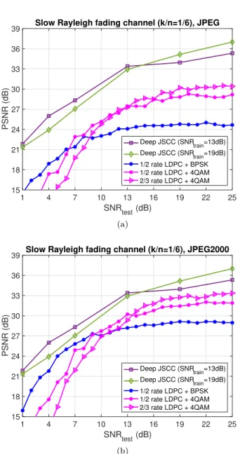
We next evaluate the performance of our deep JSCC algorithm on the Kodak image dataset over time-varying channels. Fig. 9 depicts the performance of deep JSCC and the benchmark digital transmission schemes in a slow Rayleigh fading channel for bandwidth compression ratio
k/n= 1/6. We set the average channel gain toHc = 1 and
vary the average SNR by varying the noise power σ2. In
these simulations, we assume that, in both the proposed scheme and the baseline digital transmission schemes, the phase shift introduced by the fading channel is known at the receiver, making the model equivalent to a real fading channel with double the bandwidth as only the channel gain changes randomly for each image transmission pe-riod. For the sake of readability, we only keep the best performing digital transmission schemes among all
possi-ble combinations of 1/2, 2/3 and 1/3 rate LDCP codes
and BSPK, 4-QAM, 16-QAM and 64-QAM modulation schemes. We can observe that due to the sensitivity of digital transmission schemes to the varying channel error rate as a result of varying channel SNR, the performance of the digital schemes that use separate source compression with JPEG/JPEG2000 followed by channel coding and modulation, is inferior to the performance of the proposed deep JSCC. While the digital transmission schemes per-form well only in channel conditions for which they have been optimized, our deep JSCC scheme is more robust to channel quality fluctuations. Despite being trained for a specific average channel quality, deep JSCC is able to learn robust coded representations of the images that are resilient to fluctuations in the channel quality. The latter property is highly advantageous when transmitting over time-varying channels or to multiple receivers with different channel qualities.
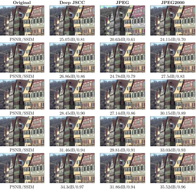
Finally, a visual comparison of the reconstructed im-ages for the source and channel coding schemes under consideration in AWGN channels is presented in Figs. 10 and 11. For the digital transmission schemes deploy-ing JPEG/JPEG2000, the images are transmitted usdeploy-ing the best-performing separate source and channel coding scheme for the target SNR value. Each row corresponds to a different channel SNR value starting from low SNR at the top (1dB) and progressing to high SNR (19dB) at the bottom. For each reconstruction, we report the PSNR and the SSIM [36] values. Fig. 10 illustrates an example where the deep JSCC outperforms the best performing digital scheme that deploys JPEG for source compression in terms of PSNR. More interestingly, although deep JSCC presents worse performance in terms of PSNR when compared to the separate scheme employing JPEG2000, its SSIM
val--2 1 4 7 10 13 16 19 22 25 SNRtest (dB) 19 21 23 25 27 29 31 33 35 37 39 PSNR (dB)
AWGN channel (k/n=1/6), JPEG
Deep JSCC (SNRtrain=-2dB) Deep JSCC (SNR train=1dB) Deep JSCC (SNR train=4dB) Deep JSCC (SNR train=7dB) Deep JSCC (SNR train=13dB) Deep JSCC (SNRtrain=19dB) 1/2 rate LDPC + 4QAM 2/3 rate LDPC + 4QAM 1/3 rate LDPC + 4QAM 1/2 rate LDPC + 16QAM 2/3 rate LDPC + 16QAM 1/2 rate LDPC + 64QAM 2/3 rate LDPC + 64QAM (a) -2 1 4 7 10 13 16 19 22 25 SNRtest (dB) 18 20 22 24 26 28 30 32 34 36 38 40 42 PSNR (dB)
AWGN channel (k/n=1/6), JPEG2000
Deep JSCC (SNR train=-2dB) Deep JSCC (SNR train=1dB) Deep JSCC (SNR train=4dB) Deep JSCC (SNR train=7dB) Deep JSCC (SNR train=13dB) Deep JSCC (SNR train=19dB) 1/2 rate LDPC + BPSK 1/2 rate LDPC + 4QAM 2/3 rate LDPC + 4QAM 1/3 rate LDPC + 4QAM 1/2 rate LDPC + 16QAM 2/3 rate LDPC + 16QAM 1/2 rate LDPC + 64QAM 2/3 rate LDPC + 64QAM (b)
Fig. 8. Performance comparison of deep JSCC with baseline digital transmission schemes on the Kodak image dataset over AWGN channels with bandwidth compression ratiok/n= 1/6. The digital schemes employ (a) JPEG and (b) JPEG2000 for image compression and various channel codes and modulation schemes.
ues are consistently higher, indicating superior perceived visual quality. Fig. 11 shows an example where for high SNR values the digital transmission schemes outperform deep JSCC in the PSNR metric, but deep JSCC can still achieve comparable SSIM values when compared to the scheme using JPEG. We can see that JPEG produces visible blocking artefacts, especially in channels with low SNR, which are not present in the images transmitted with deep JSCC. The noise introduced by deep JSCC appears to be smoother than the noise of JPEG thanks to the direct mapping of source values to soft channel input values. Note that the deep JSCC can also be trained with SSIM as the loss function, which can further improve its performance in terms of the SSIM metric.
C. Computational complexity
In this section, we provide a brief discussion of the computational complexity of the proposed JSCC algo-rithm. Let us first consider the proposed encoder/decoder network. The most computationally costly operations in the encoder/decoder are the 2D convolutions/transpose convolutions, as they involve multiplications and
addi-1 4 7 10 13 16 19 22 25 SNRtest (dB) 15 18 21 24 27 30 33 36 39 PSNR (dB)
Slow Rayleigh fading channel (k/n=1/6), JPEG
Deep JSCC (SNRtrain=13dB) Deep JSCC (SNR train=19dB) 1/2 rate LDPC + BPSK 1/2 rate LDPC + 4QAM 2/3 rate LDPC + 4QAM (a) 1 4 7 10 13 16 19 22 25 SNRtest (dB) 15 18 21 24 27 30 33 36 39 PSNR (dB)
Slow Rayleigh fading channel (k/n=1/6), JPEG2000
Deep JSCC (SNRtrain=13dB) Deep JSCC (SNRtrain=19dB) 1/2 rate LDPC + BPSK 1/2 rate LDPC + 4QAM 2/3 rate LDPC + 4QAM (b)
Fig. 9. Performance comparison of deep JSCC with baseline digital transmission schemes on the Kodak image dataset over slow Rayleigh fading channels with bandwidth compression ratio k/n= 1/6. The digital schemes employ (a) JPEG and (b) JPEG2000 for image compression and various channel codes and modulation schemes.
tions. The computational cost of a single convolutional
layer isF×F×D×K×W×H [37], whereF is the filter
size, K is the number of filters,D is the number of input
channels and W ×H is the size of the feature map. The
computational complexity of the encoder/decoder network is, thus,OIWIH
whereIW andIH are the input image
width and height, respectively. This implies that the com-putational complexity of the proposed encoder/decoder is linear in the number of pixels of the input image, as only the feature map width and height depend on the image dimensions, while all other factors are constant and inde-pendent of the image size. The JPEG encoding/decoding complexity is also linear in the number of pixels [38], while LDPC codes have linear encoding/decoding times [39]. Thus, the computational complexity of a separate joint source and channel coding scheme, which employs JPEG
for compression and LDPC codes for channel coding, is also linear in the size of the input image, i.e., OIWIH
. To complete our discussion of computational complex-ity, we have measured the average run time of the pro-posed algorithm on a Linux server with eight 2.10GHz Intel Xeon E5-2620V4 CPUs and a Tesla K80 GPU. The measurements were performed on the Kodak color
images with a resolution of 768×512 pixels. The average
run time refers to the average time required to encode and decode one image using the proposed deep JSCC architecture. The average run time achieved by our GPU implementation is 18ms per image, while the average run time on CPU is 387ms. As a comparison, the average time required for the JPEG encoding and decoding of the above images, as reported in the literature, varies from 30ms [8] to 390ms [9], while for the JPEG2000 algorithm the average encoding and decoding time on these images is even higher (e.g., 430-590ms [8], [9]). This time must be further augmented by the time needed to encode/decode the compressed bitstream with a channel code. The above proves that our method is competitive with the baseline separate source and channel coding approaches not only in terms of quality, but also in terms of computational complexity.
V. Conclusions and Future Work
We have proposed a novel deep JSCC architecture for image transmission over wireless channels. In this archi-tecture, the encoder maps the input image directly to channel inputs. The encoder and the decoder functions are modeled as complementary CNNs, and trained jointly on the dataset to minimize the average MSE of the reconstructed image. We have compared the performance of this deep JSCC scheme with conventional separation-based digital transmission schemes, which employ widely used image compression algorithms followed by capacity-achieving channel codes. We have shown through exten-sive numerical simulations that deep JSCC outperforms separation-based schemes, especially for limited channel bandwidth and low SNR regimes. More significantly, deep JSCC is shown to provide a graceful degradation of the reconstruction quality with channel SNR. This observation is then used to benefit from the proposed scheme when communicating over a slow fading channel; deep JSCC performs reasonably well at all average SNR values, and outperforms the proposed separation-based transmission scheme at any channel bandwidth value.
In the case of DL-based JSCC, the encoder and decoder networks learn not only to communicate reliably over the channel (as in [11], [13]), but also to compress the images efficiently. For a perfect channel with no noise, if the source bandwidth is greater than the channel bandwidth,
i.e., n > k, the encoder-decoder NN pair is equivalent
to an undercomplete autoencoder [5], which effectively
learns the most salient features of the training dataset. However, in the case of a noisy channel, simply learning a good low-dimensional representation of the input is not
Original Deep JSCC JPEG JPEG2000 PSNR/SSIM 25.07dB/0.81 20.63dB/0.61 24.11dB/0.70 PSNR/SSIM 26.86dB/0.86 24.78dB/0.79 27.5dB/0.83 PSNR/SSIM 28.45dB/0.90 27.14dB/0.86 30.15dB/0.89 PSNR/SSIM 31.46dB/0.94 29.81dB/0.91 33.03dB/0.93 PSNR/SSIM 34.3dB/0.97 31.86dB/0.94 35.52dB/0.96
Fig. 10. Examples of reconstructed images produced by the deep JSCC algorithm and the baseline digital schemes that use JPEG/JPEG2000 for image compression for AWGN channel and bandwidth compression ratiok/n= 1/6. From top to bottom, the rows correspond to SNR values of 1dB, 4dB, 7dB, 13dB and 19dB.
sufficient. The network should also learn to map the salient features to nearby representations so that similar images can be reconstructed despite the presence of noise. We also note that, the resilience to channel noise acts as a sort of a regularizer for the autoencoder. For example, when there is no channel noise, if the channel bandwidth is larger than the source bandwidth, i.e.,n < k, we obtain an overcomplete autoencoder, which can simply learn to replicate the image. However, when there is channel noise, even an overcomplete autoencoder learns a non-trivial mapping that is resilient to channel noise, similarly to denoising autoencoders.
The next step in improving the performance of the deep JSCC scheme is to exploit more advanced NN architec-tures in the autoencoder that have been shown to improve the compression performance [6], [40]. We will also explore
the performance of the system for non-Gaussian channels as well as for channels with memory, for which we do not have capacity-approaching channel codes. We expect that the benefits of the proposed NN-based JSCC scheme will be more evident in these non-ideal settings.
References
[1] T. M. Cover and J. A. Thomas,Elements of Information The-ory. Wiley-Interscience, 1991.
[2] F. Zhai, Y. Eisenberg, and A. K. Katsaggelos, “Joint source-channel coding for video communications,” in Handbook of Image and Video Processing, 2nd ed., A. Bovik, Ed. Burlington: Academic Press, 2005.
[3] Google, “WebP compression study.” [Online]. Available: https: //developers.google.com/speed/webp/docs/webp study [4] Y. Bengio, “Learning deep architectures for AI,” Found. and
Trends in Machine Learning, vol. 2, no. 1, pp. 1–127, Jan. 2009. [5] I. Goodfellow, Y. Bengio, and A. Courville,Deep learning. MIT
Original Deep JSCC JPEG JPEG2000 N/A PSNR/SSIM 30.69dB/0.87 22.68dB/0.67 PSNR/SSIM 31.92dB/0.89 31.65dB/0.86 36.40dB/0.92 PSNR/SSIM 32.90dB/0.90 34.36dB/0.91 38.46dB/0.94 PSNR/SSIM 35.34dB/0.93 36.45dB/0.93 40.5dB/0.96 PSNR/SSIM 36.83dB/0.94 37.79dB/0.95 41.96dB/0.96
Fig. 11. Examples of reconstructed images produced by the deep JSCC algorithm and the baseline digital schemes that use JPEG/JPEG2000 for image compression for AWGN channel and bandwidth compression ratiok/n= 1/12. From top to bottom, the rows correspond to SNR values of 1dB, 4dB, 7dB, 13dB and 19dB.
[6] J. Balle, V. Laparra, and E. P. Simoncelli, “End-to-end opti-mized image compression,” inProc. of Int. Conf. on Learning Representations (ICLR), Apr. 2017, pp. 1–27.
[7] L. Theis, W. Shi, A. Cunnigham, and F. Husz´ar, “Lossy image compression with compressive autoencoders,” inProc. of the Int. Conf. on Learning Representations (ICLR), 2017.
[8] O. Rippel and L. Bourdev, “Real-time adaptive image compres-sion,” inProc. Int. Conf. on Machine Learning (ICML), vol. 70, Aug. 2017, pp. 2922–2930.
[9] Z. Cheng, H. Sun, M. Takeuchi, and J. Katto, “Deep convolu-tional autoencoder-based lossy image compression,” inProc. of Picture Coding Symposium (PCS), San Francisco, CA, 2018, pp. 253–257.
[10] T. J. O’Shea, K. Karra, and T. C. Clancy, “Learning to commu-nicate: Channel auto-encoders, domain specific regularizers, and attention,” inProc. of IEEE Int. Symp. on Signal Processing and Information Technology (ISSPIT), Dec. 2016, pp. 223–228. [11] T. O’Shea and J. Hoydis, “An introduction to deep learning for the physical layer,”IEEE Transactions on Cognitive Commu-nications and Networking, vol. 3, no. 4, pp. 563–575, Dec 2017. [12] H. Kimet al., “Communication algorithms via deep learning,” in Proc. of Int. Conf. on Learning Representations (ICLR), 2018.
[13] E. Nachmaniet al., “Deep learning methods for improved decod-ing of linear codes,”IEEE Journal of Selected Topics in Signal Processing, vol. 12, no. 1, pp. 119–131, Feb 2018.
[14] A. Caciularu and D. Burshtein, “Blind channel equalization using variational autoencoders,” in Proc. IEEE Int. Conf. on Comms. Workshops, Kansas City, MO, May 2018, pp. 1–6. [15] T. J. O’Shea, T. Erpek, and T. C. Clancy, “Deep learning based
MIMO communications,”arXiv:1707.07980 [cs.IT], 2017. [16] A. Felix, S. Cammerer, S. Dorner, J. Hoydis, and S. ten Brink,
“OFDM autoencoder for end-to-end learning of communications systems,” inProc. IEEE Int. Workshop Signal Proc. Adv. Wire-less Commun. (SPAWC), Jun. 2018.
[17] H. Ye, G. Y. Li, and B. Juang, “Power of deep learning for channel estimation and signal detection in OFDM systems,” IEEE Wireless Communications Letters, vol. 7, no. 1, pp. 114– 117, Feb. 2018.
[18] N. Farsad, M. Rao, and A. Goldsmith, “Deep learning for joint source-channel coding of text,” in Proc. IEEE Int. Conf. on Acoustics, Speech and Signal Processing (ICASSP), Apr. 2018. [19] R. Zarcone et al., “Joint source-channel coding with neural networks for analog data compression and storage,” in 2018 Data Compression Conference, March 2018, pp. 147–156.
[20] A. Ignatovet al., “AI benchmark: Running deep neural networks on android smartphones,” inComputer Vision – ECCV 2018 Workshops, L. Leal-Taix´e and S. Roth, Eds. Cham: Springer, 2019, pp. 288–314.
[21] R. A. Solovyev, A. A. Kalinin, A. G. Kustov, D. V. Telpukhov, and V. S. Ruhlov, “FPGA implementation of convolutional neural networks with fixed-point calculations,” CoRR, vol. abs/1808.09945, 2018.
[22] A. G. Fabregas, A. Martinez, and G. Caire, “Bit-interleaved coded modulation,”Foundations and Trends in Communica-tions and Information Theory, vol. 5, no. 1-2, pp. 1–153, 2008. [23] N. Thomos, N. V. Boulgouris, and M. G. Strintzis, “Optimized transmission of JPEG2000 streams over wireless channels,” IEEE Trans. on Image Processing, vol. 15, no. 1, pp. 54–67, Jan 2006.
[24] D. Gunduz and E. Erkip, “Joint source-channel codes for MIMO block-fading channels,”IEEE Trans. on Information Theory, vol. 54, no. 1, pp. 116–134, Jan 2008.
[25] I. Kozintsev and K. Ramchandran, “Robust image transmission over energy-constrained time-varying channels using multires-olution joint source-channel coding,” IEEE Transactions on Signal Processing, vol. 46, no. 4, pp. 1012–1026, April 1998. [26] T. Goblick, “Theoretical limitations on the transmission of
data from analog sources,”IEEE Transactions on Information Theory, vol. 11, no. 4, pp. 558–567, October 1965.
[27] S. Jakubczak and D. Katabi, “SoftCast: Clean-slate scalable wireless video,” inProc. of the 48th IEEE Annual Allerton Conf. on Communication, Control, and Computing, Illinois,USA, Sept. 2010, pp. 530–533.
[28] T. Tung and D. Gunduz, “Sparsecast: Hybrid digital-analog wireless image transmission exploiting frequency-domain spar-sity,”IEEE Communications Letters, vol. 22, no. 12, pp. 2451– 2454, Dec 2018.
[29] D. Alexandre, C.-P. Chang, W.-H. Peng, and H.-M. Hang, “An autoencoder-based learned image compressor: Description of challenge proposal by nctu,” inIEEE Conf. Comp. Vision and Pattern Recog. Works., Jun. 2018.
[30] K. He, X. Zhang, S. Ren, and J. Sun, “Delving deep into recti-fiers: Surpassing human-level performance on imagenet classifi-cation,”arXiv:1502.01852v1 [cs.CV], 2015.
[31] M. Abadiet al., “TensorFlow: Large-scale machine learning on heterogeneous systems,” software available from tensorflow.org. [Online]. Available: https://www.tensorflow.org/
[32] D. P. Kingma and J. Ba, “Adam: a method for stochastic optimization,”arXiv:1412.6980 [cs.LG], 2014.
[33] A. Krizhevsky, “Learning multiple layers of features from tiny images,” University of Toronto, Tech. Rep., 2009.
[34] Y. Polyanskiy, H. V. Poor, and S. Verdu, “Channel coding rate in the finite blocklength regime,”IEEE Transactions on Information Theory, vol. 56, no. 5, pp. 2307–2359, May 2010. [35] J. Deng et al., “ImageNet: A Large-Scale Hierarchical Image
Database,” inCVPR09, 2009.
[36] Z. Wang, A. C. Bovik, H. R. Sheikh, E. P. Simoncelli et al., “Image quality assessment: from error visibility to structural similarity,”IEEE Transactions on Image Processing, vol. 13, no. 4, pp. 600–612, 2004.
[37] A. G. Howardet al., “Mobilenets: Efficient convolutional neural networks for mobile vision applications,”arXiv:1704.04861v1 [cs.CV], 2017.
[38] P. T. Chiou, Y. Sun, and G. S. Young, “A complexity analysis of the JPEG image compression algorithm,” in Proc. of 9th Computer Science and Electronic Engineering (CEEC), Sep. 2017, pp. 65–70.
[39] T. Richardson and R. Urbanke,Modern Coding Theory. New York, NY, USA: Cambridge University Press, 2008.
[40] N. Johnston et al., “Improved lossy image compression with priming and spatially adaptive bit rates for recurrent networks,” in The IEEE Conference on Computer Vision and Pattern Recognition (CVPR), June 2018.
Eirina Bourtsoulatze[S’11 - M’14] received the Diploma in Electrical and Computer Engi-neering from the Aristotle University of Thes-saloniki, Greece, in 2008 and the Ph.D. de-gree in Electrical Engineering from the Ecole Polytechnique F´ed´erale de Lausanne (EPFL), Switzerland, in 2013. She is currently a Marie Curie Research Fellow in the Department of Electronic and Electrical Engineering of Uni-versity College London, UK. Her research in-terests include machine learning for communi-cations, image/video processing, information-centric networks, net-work coding and multimedia communications.
David Burth Kurka [S’14] received Eng. and M.S. degrees in Computer Engineering from University of Campinas, Brazil in 2015. He is currently a PhD student in the Electrical and Electronic Engineering Department of Im-perial College London. His research interests include machine learning for communications, multi-agent systems and socially inspired com-puting. His PhD research is funded by the Na-tional Council for Scientific and Technological Development (CNPq), Brazil.
Deniz G¨und¨uz [S’03 - M’08 - SM’13] re-ceived the M.S. and Ph.D. degrees in electrical engineering from NYU Polytechnic School of Engineering (formerly Polytechnic University) in 2004 and 2007, respectively. He is currently a Reader in the Electrical and Electronic Engi-neering Department of Imperial College Lon-don. His research interests lie in the areas of communications and information theory, ma-chine learning, and privacy. He is the recipient of the IEEE Communications Society - Com-munication Theory Technical Committee (CTTC) Early Achieve-ment Award in 2017 and a Starting Grant of the European Research Council (ERC) in 2016.