Dynamic characteristics of a hyperboloid shell of revolution with application to flexible couplings

Rochester Institute of Technology

RIT Scholar Works

Theses

Thesis/Dissertation Collections

7-2005

Dynamic characteristics of a hyperboloid shell of

revolution with application to flexible couplings

Brian G. Towner

Follow this and additional works at:

http://scholarworks.rit.edu/theses

This Thesis is brought to you for free and open access by the Thesis/Dissertation Collections at RIT Scholar Works. It has been accepted for inclusion in Theses by an authorized administrator of RIT Scholar Works. For more information, please [email protected].

Recommended Citation

Dynamic Characteristics of a Hyperboloid Shell of

Revolution with Application to Flexible Couplings

Approved by:

Dr. Hany Ghoneim

By

Brian G. Towner

A Thesis Submitted in

Partial Fulfillment of the

Requirement for the

MASTER OF SCIENCE

IN

MECHANICAL ENGINEERING

Hany Ghoneim

Department of Mechanical Engineering

(Thesis Advisor)

Dr. JosefT6r6k

Department of Mechanical Engineering

Dr. Kevin Kochersberger

Department of Mechanical Engineering

Dr. Edward C. Hensel

Department Head of Mechanical Engineering

J.

S. Torok

Kevin Kochersberger

Edward Hensel

I, Brian G

.

Towner, hereby grant permission to reproduce my thesis in whole

or in part. Any reproduction will not be for commercial use or profit.

Date:

0

t":f/d..

q

1

0

5

I

I

Rochester

Institute

of

Technology

Abstract

Dynamic Characteristics

of a

Hyperboloid Shell

ofRevolutionwith

Application

to

Flexible Couplings

Brian G. Towner

Advisor: Dr.

Hany

Ghoneim

Ahyperboloidshell of revolution

(HSR)

isproposedfor implementationas a_coupling,

into a

fully

integrated

driveshaft/coupling

assembly.Thedynamicsofthe_{coupling is}not

clearlyunderstood;whichpromptstheneed forananalyticinvestigationofthe hyperboloidshellofrevolution.

Thehyperboloid shell ofrevolutionisoneinwhichthemeridianoftheshellis defined

by

the equation of ahyperbola. Twomethods are utilizedtofindthefirst

bending frequency

oftheHSR: Finite Element MethodandtheAssumed Mode Shape Method. The Finite

Element Method is appliedto Timoshenko Beam

Theory,

andGalerkin's Assumed Mode

Shape Method isappliedto the Kirchoff-Love

theory

ofthinshells. Bothmethods are

TABLE OF

CONTENTS

Page

CHAPTER

1:

INTRODUCTION

1

1.1

INTRODUCTION

1

1.1.1 COUPLINGOVERVIEW 1

1.1.2 TYPES OF COUPLINGS 2

1.1.3 COUPLINGSAND DRIVESHAFTS 3

1.1.4 APPLICATION OF COMPOSITES 4

1.2 DRIVESHAFT COUPLING ASSEMBLIES 7

1.2.1 GEISLINGER GESILCO ADVANCED COMPOSITE 7

1.2.2 INTEGRAL COMPOSITE SHAFT-COUPLING 10

1.2.3 COOLING TOWER COUPLING 12

1.2.4 LAWRIE DRIVESHAFT COUPLING 14

1.3 REVIEW OF HYPERBOLA 16

1.4 OTHER APPLICATIONS 16

1.5 PARAMETRIC STUDY 18

CHAPTER2:ANSYSMODEL 20

2.1 MODELING THE SHELL 20

2.2 RESULTS 23

2.2.1 DYNAMIC RESULTS 23

2.2.2 STATIC RESULTS 26

CHAPTER 3: TIMOSHENKOBEAM THEORY 29

3.1 MATHEMATICALMODEL 29

3.2 FINITE ELEMENT FORMULATION 31

3.3 RESULTS 35

CHAPTER4: SHELLTHEORY 38

4.1 METHEMATICAL MODEL 38

4.1.1 KIRCHOFF-LOVEASSUMPTIONS 38

4.1.2 MATHEMATICAL MODEL OF ASHELLOF

REVOLUTION

39

4. 1.2.A KINEMATICS 40

4.1.2.C FORCE AND MOMENT EXPANSION 43

4.1.2.D EQUILIBRIUM EQUATIONS 45

4. 1.3 MATHEMATICALMODEL OF THE HYPERBOLOID SHELL

OF REVOLUTION 47

4. 1.3.A KINEMATICS 47

4.1.3.B EQUILIBRIUM EQUATIONS 49

4.2 SOLUTION 52

4.2. 1 INTRODUCTION TO THE GALERKTN ASSUMED MODE

SHAPE METHOD 52

4.2.2 APPLICATION OF THE GALERKTN ASSUMDED MODE SHAPE

METHOD 53

4.3 RESULTS 57

CHAPTER5: RESULTSCOMPARISON 60

CHAPTER 6:CONCLUSION/FUTURE WORK 64

REFERENCES 66

APPENDIX A: HELPFUL TABLES 68

APPENDIX B: ANSYSBATCH FILES 70

APPENDIXC: MAPLEANDMATLABFILES 93

APPENDIX D: EXPANDED FORCES ANDMOMENTS 100

APPENDIXE: EXPANDED MATRIXELEMENTS 101

APPENDIX F: MATHEMATICAFILES 107

LIST

OF FIGURES

Figure Page

Figure 1.1: Three Typesof

Flexibility

[1]

1

Figure 1.2:DirectionsrelativetoComposite Fibers

[4]

6

Figure 1.3: Geislinger Gesilco Cl-design

[7]

8

Figure 1.4: B-F Design

Coupling

[7]

8

Figure 1.5: BI-Design

Coupling

[7]

9

Figure 1.6: An integral compositedriveshaft

coupling

[5]

10

Figure 1.7: Schematicof aComposite

Cooling

Tower

Coupling

[9]

13

Figure 1.8: Schematicof anIntegrated

Shaft-Coupling Assembly

14

Figure 1.9: Geodesic LinesoftheHSR 15

Figure 1.10:

Geometry

(c &

d)

defining

aHyperbola 16

Figure 1.11:

Geometry

oftheParametric

Study

18

Figure 2.1: Figure 2.1: HSR Model Generated

by

ANSYS 21

Figure 2.2: The ANSYS Finite Element MeshofHSR 22

Figure 2.3: Ratioc/d vs. Natural

Frequency

for Fixed-Free HSR

(ANSYS)

23

Figure 2.4: Minimum Radius vs.

Frequency

for Fixed-Free HSR

(ANSYS)

24

Figure 2.5: Minimum Radius vs.First

Bending Frequency

for Fixed-Fixed

HSR

(ANSYS)

25

Figure 2.6: Minimum Radius vs.

Bending

Stiffness Results 26

Figure 2.7: Minimum Radiusvs.Torsional Stiffness 27

Figure 2.8: Minimum Radiusvs. AxialStiffness 27

Figure 3.1: Timoshenko Beam Differential Element 29

Figure 3.2: Fixed-Free Results

by

TimoshenkoBeamandFinite Elements 36

Figure 3.3: Fixed-FixedResults

by

Timoshenko BeamandFinite Elements 37

Figure 4.1: CoordinatesofShell

[10]

41

Figure 4.2: DifferentialElementandStress 41

Figure4.3: Differential ElementwithUnitForces andMoments 43

Figure 4.5:

Bending

Natural Frequencies of aFixed-Free HSR

by

Applying

theGalerkin MethodtoShell

Theory

58

Figure 4.6:

Bending

Natural Frequencies of aFixed-FixedHSR

by

Applying

theGalerkin MethodtoShell

Theory

59

Figure 5.1:Fixed-FreeResults Comparison: ANSYS vs.TimoshenkoBeamvs.

Shell

Theory

61

Figure5.2:Fixed-Fixed Results Comparison: ANSYSvs. Timoshenko Beamvs.

LIST OF

TABLES

Table Page

Table 5.1:Fixed-Free Results Comparison 60

NOMENCLATURE

A Area.

C Membrane Stiffness.

D

Bending

Stiffness.

c&d Parameters

Defining

thehyperbola.

E Young's Modulus.

fn

Natural

Frequency

(Hz).

G Shear Modulus.

h ThicknessofShell.

I MomentofInertia.

K

Curvature.

Kg

Gaussian Curvature.

M Moment.

R>

Distance_{to the meridian;}perpendicularto thecenterline.

Ri

Radiusof circumferentialcurvature.

R2

Radiusofmeridional curvature.

u,v,w Localdisplacementsofshell.

Ul,U2,Z Localcoordinate systemofshell.

V Shear.

e Strain.

P Density.

a Stress.

v Poisson's Ratio.

Chapter

1:

INTRODUCTION

1.1

INTRODUCTION

1.1.1

COUPLING

OVERVIEW

Inmost practicalapplicationsperfect alignmentof couplings_{to machines,} and/orshafts is

impossible.

Misalignmentscan occurbecauseof severalreasons including: thermal

expansion,

installation

error,deflectioncaused

by

applied

loads,

andwearofbearingsand

machine parts. These misalignments causehighreaction

forces,

whichresultin_vibration,

noise,

bearing

failureand sometimesfailureof shafts. Thethreemainformsof misalignment [image:11.540.150.374.368.453.2]

are_angular, axial andlateral

[1]

as seenin Figure 1.1.

Figure 1.1: Three Typesof_Flexibility[1].

Themostbasic wayof_connectingtwomachines or shaftsis

by

meansofarigid coupling.

Rigidcouplingscantransmit torqueand axialthrustbutare unabletohandle_anyofthe

misalignments_previouslymentioned. Ifmisalignments_exist, rigidcouplings can generate

highreaction forces. Thesereactionforces_{may induce noisy operation,} increased_vibrations,

Duetomisalignment theneedarises fortheuse offlexiblecouplings, whichmustbeableto

transmit power and accommodatethemisalignments[2]. The flexiblecouplings must also be

abletooperate athigh_speeds, andhandle

loads,

caused

by

acceleration and

deceleration,

while

transmitting

powerandtorque.

They

mustalsobeabletocompensateformovementof

the shaft,which oftenis inthe formof vibrations [3].

1.1.2

TYPES

OF COUPLINGS

According

to Johnson

[1],

flexiblecouplings_{generally fall}undertheone offourcategories.

Thesecategoriesare: Mechanical

Flexible, Elastomeric,

Metallic

Membrane,

and

Miscellaneous. Mechanicalflexiblecouplings arecategorized

by

loose

fitting

_parts,and/or

the_rollingor_slidingof_{parts, to}givethe_{coupling its} flexibility. _{This category}ofcouplings

includesbut isnotexclusivetogear_couplings, chain andsprocket _couplings,grid _couplings,

andthebasic U-joint. Mechanical flexiblecouplings_{may have}ahigh initial_cost, andmost

require

lubrication,

whichisa majordisadvantageofthis typeof_coupling

[1,

3]. Elastomeric

couplings gaintheir

flexibility by

deformationof resilient elastic_materials,

including

plastics

and rubbers.

They

_generallyfallunderoneoftwo categories: couplingsthat transmit torque

in shear, andthose thattransfertorqueincompression. Acommoncompressiontypeis a

Spyder/Jawcoupling, and acommonsheartypeis aTyrecoupling. Other Elastomeric

couplings include: donut-typecouplings, pin and

bushing

_couplings,andelastomericblock

coupling. Dueto theelastomeric material_properties,couplingsthat functionincompression

vibrationdamping. Ametallic membrane_{coupling is}either made_upofmetallicdiscsor uses

a metallicdiaphragmto gaintheir flexibility. Thedisctype_couplinguses oneor more

discs,

which are_alternatelyattachedto eachotherand/orinput and outputflanges. The diaphragm

type_couplingtakesadvantageofaflexiblemetal elementconcentricallyattachedto two

flanges

[1,

3]. Themetallic membrane_{coupling holds}several advantages.

They

do not

require

lubrication,

they

are_{relativelytolerant to chemicals,} and

they

havea

long

lifeand

tendnottowearlikeother couplingsbecauseoftheirlackof_slidingcontact

[1,

2]. The

diaphragmtypecouplings accommodate axial angular andlateralmisalignments

depending

onthedesign.

Compositeshave beenusedinsimilarapplicationstometallic membrane couplings.

Composite disccouplingstakeadvantage of a pack ofdiscs made of composite materials.

Thecomposite material allowsthe_couplingto haveahightorsional_stiffness,offershigher

misalignmentthana similarmetallicdisc_{type coupling,} and also offers good

damping

[1,3].

1.1.3

COUPLINGS AND DRIVESHAFTS

Modernenginesandtransmissions testthecapabilities ofdrive shaftsandcouplings [5].

Machines are

being

_produced,whichare_operatingathigherspeeds andare_operatingmuch

closerto thenatural frequenciesoftheshafts and/or couplings[2]. Shaft and_coupling

combinations mustbe abletohandlemisalignments while

being

abletooperate athigh

speeds, and

they

mustbelight inordertooperateathighnatural

frequency

requirements

[3,

5].

Along

with_{the previously}mentionedrequirements;

they

must also_{be aesthetically}

Forinitialanalysis of adriveshaft_simplysupported

boundary

conditionscanbeassumed.

By

simulations it isobviousthat theshaft

by

itselfdoesnotdeterminethenaturalfrequency.

Motionoccurs attheattachment points_{corresponding}to thecouplings [5]. These_motions,

oftenbecauseof_{misalignments,} causesignificant reactionforcesontheshaft [1]. These

forcesare a result ofthestiffnessof_{the coupling,} andtherefore thestiffness mustbe found.

1.1.4 APPLICATION OF COMPOSITES

Thecombinationoftwoor more

distinctly

differentmaterials into anew materialis

considered acomposite material. Oneofthematerials is_usuallyafiber. Fibersare often

madeofglass or _carbon,which are _{considerably strong}and oftenhavemuchfewer defects in

fiber formthanin bulkform. Thefibersarewhat givethecomposite material muchbetter

stiffnesstoweightratiosthanothermaterials[12]. Fibersare_{very strong in}tensionandare

themaincontributorto theultimate performance of_{the composite,}but

they

alone are

insufficienttohandlecompression ortransverseloads. A

binder,

called_{the matrix,} isusedto

holdthefibers together, and moldthefibers into acomposite component. Itisoften made_up

of a

thermosetting

resin, whichincludespolyester and vinylesterresins andepoxies. The

matrixhas bothadhesive and cohesivepropertiesthat allowloadstobetransferredbetween

the fibers. Thematrixisalso importantin protectingthefibers fromtheenvironment and

givingthecomposite resistancetocorrosion

[4,

12].

Thefibersandthe matrixarebothimportantto thefinalcomposite component whileeach

Composite

technology

_{is growing rapidly in}thepowertransmission

industry,

_mainlybecause

ofits _{advantages over metals.} Whencompared_{to metals,} compositeshave higherspecific

strength and specific_stiffness, have littletono_{thermal expansion,} and areresistantto

corrosion[12].

They

also allowfor_engineering

tailoring

ofa

design,

_simply

by

_changingthe

orientation angleofthefibers. Thisallows aparttobedesignedwithdesireddynamic

characteristics. Composites' higherspecificstiffness results in highernaturalfrequencies

[6]. Thisallowsforpartstobe designed withamuchlargerrange of operation. Dueto these

advantages, someofthefirstapplicationsof composites wereintheaerospace and _cooling

tower-coupling

industries,

and now are

finding

their_wayinto commercial industry. These

advantageshave leadto theuseof compositesin driveshafts and make composites agood

materialforusein flexiblecouplings [4].

Theuniqueproperties of composites arethesame propertiesthatmaketheiranalysis

difficult.

Materials,

suchas_metals,havemechanical propertiesthatareisotropic. Materials

thatareisotropic havemechanical propertiesthat areindependentofthedirectionconsidered.

Composites are consideredtobeanisotropic;

therefore,

themechanical properties ofa

compositedependonthedirection considered. Thisphenomenonis dueto the make_upofa

composite material. Considera single

layer,

or

lamina,

ofafibrouscomposite_material

where fibersareimbeddedparallelto thex-axis intoamatrix. Thelaminawillhave a much

greater resistanceto

loading

in_{the x-direction, than}inthe_yor_z-direction,dueto thefactthat

thefiberswillbeaxial

loaded;

_therefore,themodulus of_elasticitywillbemuchhigher inthe

x-direction(or longitudinal

direction)

thaninthe_yor z-direction(or transverse

direction)

TRANSVERSE

LONGITUDINAL

Figure 1.2: DirectionsrelativetoComposite Fibers [4].

Sincethestrengthofthelaminaismuchless inthe transversedirections alaminateneedsto

becreated. Alaminate iscreated

by

_{stacking lamina}withdifferentfiberorientations. Now

thecomposite_{may handle}loadsinthedesired directions [12]. It is importanttonotethat

by

designonedirection may bestrongerthananotherbut for stabilityand_rigidityofthefinal

part, alldirectionwillhave some strength. It isthe_abilityto arrangethefibers indifferent

ways thatmakes composites unique. Thestrength and overall characteristics ofthefinal

product canbealtered

by

_arrangingthe layersofthecompositeatdifferentangles [4]. These

anisotropic propertiesthatresult fromthedifferentarrangements oflayers are whatallowus

totailor the designtomeettherequirements oneis

looking

for [1 1].

Laminateplate

theory

isthecornerstone of

theory

and analysis ofcomposites. This

theory

relates thestiffness and strain of eachlayertoproperties ofthefinallaminate. Asinglelayer

orlaminacanbe defined

by

properties found analyticallyor

by

experimentation. Then

by

rigorousmathematical

theory

thedifferentpropertiesofthematrix canbe found. Thestrain

1.2

DRIVESHAFT COUPLING

ASSEMBLIES

1.2.1 GEISLINGER GESILCO

ADVANCED COMPOSITE

TheGeislinger Gesilco advanced composite coupling, is verysimilarto ametallicdiaphragm

coupling. Geislingerwasthe firstto produce acomposite misalignment _couplingtobeused

inthe_shippingindustry. Thisapplicationisforuseon_{ship drive lines between}engine and

gears,orbetweengears and water-jet. Theirgoalwastoproducea_couplingthatwouldbe

first

torsionally

stiff, as well_as,beabletohandle highmisalignments.

Also,

this_{coupling is}

meanttohavegood soundinsulationand reducethedeadweight ofthe_couplingandinturn

reducethemass momentofinertia. Ifthe_couplingcould meettheserequirementsitwould

help

meettheneeds ofthe_shipping

industry

that thriveson weight savings. Themore weight

thatcanbesavedthemore payloads canbecarried andthefastertheshipscantravel [7].

A verygooddesignoverviewis giveninthepaperin its General Design Concept section.

Thecomposite _{coupling is}a membrane_{coupling designed}tomeet several requirements.

Someoftherequirementsinclude:

being

abletooperatebetween 100and 3000_rpm,

having

at leasta20000 hourservice

life,

mustbeabletohandleatorqueof

300kNm,

and mustbe

abletohandlea3 degreeangleofdeflection [7]. Itis importanttonotethat this isnot an

integralcomposite shaft _couplingassembly.

Therearetwomain _coupling

designs,

aswell_as, a combinationofthe twodesigns. Thefirst

design,

the

Cl-design,

ismade_upoftwo membranes anda shaft attheinner diameterofthe

membranes. AdiagramoftheCl-designis shownin Figure 1.3. Themembranes are

1

Figure13: Geislinger Gesilco Cl-design [7].

The second

design,

the

BF-(Butterfly)-design,

consists ofintermediateshafts arranged onthe

outerdiameterofthemembranes. Thetwohalvesofthe_couplingcanthenbeboltedtogether

anddifferent sizedwashers canbeused to

help

compensatefor anyaxialmisalignment.

Figure 1.4: BF-Design_Coupling[7J.

Acombinationofthe two couplingsiscalledtheBl-design. Themain advantage ofthe

BI-designallows _{the coupling to}beattachedtotheengines flywheel

by

theCl-part andto a [image:18.540.186.352.83.183.2] [image:18.540.194.349.341.474.2]

[image:19.540.221.336.54.205.2]

Figure 1.5: BI-Design

Coupling

[7].

The composite_couplingismade

by

meansoftheprepeg/auto clave _{manufacturing}technique.

Thismethod was chosenbecause itoffered good_{reproducibility}and it isableto yield ahigh

fibervolume contents. Eachlayerofthelaminate is_made-upofE-glassorcarbon

unidirectional_prepregtapes. Thedesignofthecomposite membraneusedinthecouplingsis

unique. Thecross-section ofthemembraneistapers towards theouterdiameterandis

corrugated. Itwasfound

by

simulation and experimentationthat thisdesignyields ahigher

deflectionwithlowerstiffnessthanaflattaperedmembrane. Thelowerstiffness yields

muchlowerreaction forces [7].

Thedesignerofthe_{coupling decided using finite}element _analysis,

by

meansofthe

simulation program

ANSYS,

andwas asuitabletool foranalysis. Theauthordidmention

that thereisaneedfora_good,reliable means of analysisfora composite membrane loaded

inthismanner. Theresultswerelatercompared against experimentaldata. Acoupleof

assumptionswereusedintheanalysis.

First,

itwasassumedthatinthemodelthesingle

seemstocorrespond _{closelyto the}FEAresults it is possibletooptimizethecomposite

couplingusingtheFEAmodels [7].

Since 1993 morethan500 ofthesecouplingshave been inservice. Theoldest_{coupling has}

been running forover 16000hourswithnoproblems. This couplingisused on afast

ferry

thatwasbuiltinaSpanish shippingyard. Itseems so farthatdesignanddevelopment of

theseparticular composite couplingshasbeena success [7].

1.2.2 INTEGRAL COMPOSITE SHAFT-COUPLING

Apaper

by

Faust, Hogan, Margasahayam,

andHess

[5]

givesanoverviewof anintegrated

compositedriveshaft andcouplingsthatwereintheprocessof

being

developed. Theauthors

statethat the_combiningoftheshaft couplings isunusual andunique. Thepart described is

firstmadeof a shaft whichisconstructed_usingbraided-fiberglass. Thecouplingsarethen

integrally

braided intothepart.

Finally

theprocessiscompletedbemeansof resintransfer

molding. The designoftheintegralshaftand _couplingmust meet severalstrictdesign

criteria. Someofthemostcriticalareas follows. Thepartmustbeableto transmit 1200

hp

at23,000rpm,must operateintherange of1 6,000to 26,000rpm, and musthavea natural

[image:20.540.187.358.579.668.2]

Severalequations arelistedthatwereusedinthe_preliminaryanalysis

by

Faust, Hogan,

MargasahayamandHess. Theseequations includewaysof

finding

_{torsional stress,}flexural

strain,

buckling,

and

bending

stiffness. Theseequations areallbasedontheassumption of

isotropic_materials,whichleadto error when usedforcomposite materials.

Thus,

they

are

onlygiventoprovide somedirectiononhowthepart needstobelookedat.

Instead,

all

analysis is done

by

meansoffiniteelement analysis_{using PDA/PATRAN} and

MSC/NASTRAN,

and

by

testing

[5].

Ina parallelpaper

by

MargasahayamandFaust

[8],

adetailedoverview ofthe3D finite

element analysisdoneonthe_couplingisgiven. Finite element analysis was chosen_mainly

becauseofthe anisotropic nature of_composites, anddueto thefactthat thematerial

propertiesdiffer frompointtopointinthecoupling. Finiteelement analysis was also a_very

effective_wayof

finding

the

bending,

axial andtorsionalstiffnessinorderto aidinthe

critical speed calculationsoftheshaft coupling.

Using

CADAMa2D crosssectionwas

developedwhich was used asthebasis fora3D Finite Elementmodel. Dueto_symmetry

only halfofthe _{Shaft coupling}wasmodeled. Fortheactual_analysis, and for plotting

displacementand stress PDA/PATRANwas utilized. Themodelwasbroken into 8material

zonesto compensateforthe_{varying fiber}anglesin eachlamina. Themodelwasbroken into

solid,

8-node,

rectangularhexahedralelements. Solid brickelements were utilized insteadof

2Dshell elementsforseveralimportantreasons including: braided laminateis_relatively

thick,

interlaminarstresses wereofa_concern,

they

were usedtomodel each

layer,

itmakes it

concern. Thematerialpropertiesinput intotheprogramwerethecalculatedequivalent

mechanicalpropertiesofthe

laminate

[8].

Following

thefiniteelement _{analysis, tests}wereperformed onfull-scaleprototypes ofthe

shaft coupling. Theshaft_couplingwasloaded inthreeseparatetestsin

bending,

axial

tension,

andtorsion. Straingauges were placedinthemain areas ofinterest basedon

findings

ofthefiniteelement analysis[8].

Bothpapers _concerningthisshaft_couplingdiscusstheresults fromthefiniteelement

analysis and

testing,

bothofwhichfall verycloseto one another. Dynamiccharacteristics

arediscussedbutnotingreat

detail; however,

animportantnoteisthat theshaft alonedoes

notcontrolthenaturalfrequency. Insteadconsiderablemotionduetomisalignments ofthe

attachmentpointsofthecouplingstomachineshas agreat effect. Diaphragm

bending

ofthe

couplingsresults insignificant lateraland radial stiffness. Oneimportantnotiontakenfrom

thepaperisthat atthe timeoftheirdevelopment

they

hadto_relyon

testing

andcomputer

FEA,

becauseofthelackofbetteranalytical_{understanding [5].}

1.2.3

COOLING

TOWER

COUPLING

Composite driveshafts and flexiblecouplings havealsobeenused_{extensively in}the_cooling

tower

industry

[9]. Anexample isshown onFigure 1.5. Driveshafts made of composites

filament

_windingprocess.

Composites

were usedbecause

they

yieldedpartsthatwere much

lighter,

stronger, stiffer,andtheirdesignscouldbetailoredto meet specific application

requirements. Thecompositecomponents also yieldedhighertolerance to misalignments,

are more resistantto_{corrosion, causinglowerloads}on

bearings,

are moreresistantto

fatigue,

and show nothermal expansion. Thecompositespacertubesarealso ableto spanmuch

longer

distance,

_{which allowsfor usingfewer flexiblecouplings and supportbearings. These}

couplings are also ableto transmitgreatertorque than theirmetal_{counterparts,} andtherefore

canbedesignedtomeet speed requirements ratherthanstrength requirements [9]. These

couplingshaveproventobealowmaintenance solutiontoproblems associated with_cooling

towerdrivesystems [4].

ait sntatiss stoolmui

K-SOO UQHCL Fi

Figure 1.7: Schematicof aComposite

Cooling

Tower

Coupling

[9].

Thepaperthengives agooddescriptionofthe loadsthemisalignment couplings must

sustain.

First,

the _couplingmustbeabletohandlestaticand_vibratorytorque. Atthesame

time it musthandle 3typesof misalignment: axial, radial, and angular. Theangular and/or

1.2.4 LAWRIE

INTEGRAL

DRIVE SHAFT COUPLING ASSEMBLY

The Lawriedriveshaft consists of a shaftandtwoflexiblecouplings integratedintooneunit.

The integratedshaft_{coupling is}made fromcomposites and ismanufactured_using the

filament windingprocess. Flanges areattachedto _assemblyafter_{manufacturing [34]. The}

basicshapeofthe

integrated

shaft_{coupling assembly is} shownin Figure 1.8.

Figure 1.8: Schematicof anIntegrated

Shaft-Coupling

Assembly.

Similartothe_{previously described}shaft_{couplingassemblies,} it iscriticalthatthe_assembly

beabletohandlehigh

torque,

while_allowing

flexibility

in-bending. The

flexibility

is

obtained

by

meansofthe_couplingportions oftheassembly.

Thisthesis focusesonthe_couplingportionof_{the assembly,} andservesto

lay

thefoundation

forfutureworkinthis area. Itwill consider aportionofthe_couplingwhose shapeisdefined

by

ahyperboloidshellof revolution(HSR). Geodesic

lines,

made of

filaments,

createthe

shape ofthe coupling, intheassembly. Thesearestraightlinesthatdesignatetheshortest

surfacelinebetweentwopoints onthecurvedsurfaceoftheHSR. Asfilaments are added

[image:25.540.181.346.76.267.2]

Figure 1.9:GeodesicLinesoftheHSR.

Theinherent shapeofthisprocessisthatofahyperboloidshell of revolution

(HSR);

whose

meridianis defined

by

ahyperbola. Dueto theinherent _complexityofcompositesand

HSR,

thisthesiswillfocus on

finding

thedynamiccharacteristicsof athinHSR(thickness= .001

in)

madeof anisotropicmaterial.

Specifically,

thematerial chosenintheanalysisofthe

shellwas

Aluminum;

_therefore,the

following

properties were used:

p=2.55x1 0-4

lbf

s2 /in4

,

E=

10x\06psi,

1.3

REVIEW

OF

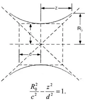
HYPERBOLA

Themeridian ofthe

hyperboloid

shell is_{naturally defined}

by

a

hyperbola,

whoseequation is [image:26.540.191.337.145.318.2]

presented _{in Figure 1.10.}

Figure 1.10:

Geometry

(c&_{d) defining}aHyperbola.

As canbeseenfromFigure 1.1

0,

canddare constantsthatdefinea rectangle whose

diagonals formtheasymptotesofthehyperbola[16].

Changing

one orbothofthesevalues

changesthe curvature ofthehyperbola. Basedonthisgeometric_{relationship, the}parametric

study, outlinedinChapter

Two,

is developed.

1.4

OTHER APPLICATIONS

Thereareother applicationto Hyperboloid Shellsof

Revolution,

including

water

towers,

TV

towers,

structuralsupports,

factory

chimneys, anddesignsofbuildings. Themost common

maybethe applicationof_coolingtowers. Thisshapewas chosenforthe_coolingtowers

Countlesspapers canbe foundontheanalysisof_coolingtowers. Thisanalysisfocuses

mainlyonthe

buckling

and vibrations ofthe_cooling towers.

Early

_work, likethatdone

by

Carter

[26]

andNeal

[25],

weredone

by

means ofbasicshell

theory

and

by

extensive

experimentation. Muchofthisresearch wasdoneininterestto failureof_coolingtowersin

the 1960s

[25,

26]. Carterexplainsthatmuchofthe_earlyexperimentation wasdonewith

insufficient

boundary

_conditions,

leading

to errorinresults. Lateranalysisof_coolingtowers

focusesontheuseofFinite ElementAnalysis. Examplesofthiswork

include,

butare not

limitedto,workdone

by

Aksu

[24],

andTan [27].

Also,

general workthatmentions

applicationtohyperboloids

includes,

butisnotisnotlimited

to,

work

by

Lee& Bathe

[30],

and

by

FanandLuah [30].

Theanalysis inthis thesis is different when comparedto analysisdoneintheprevious

mentioned papers and similarliterature. Oneoftheobviousdifferencesisthat theflexible

coupling isconsidered symmetric about whatwouldbethe_x-yplainin Figure 1.10.

Cooling

towers are_generallymuch longeron one sideofthe

throat,

wheretheminimum radiusis

located. More

importantly

no literaturecouldbe

found,

thatstudiedtheaffectsof_changing

theparametersonthenatural

frequency

ofthehyperboloid. This isthemainfocusofthis

thesisasisexplainedin Chapter Two. Theanalysis is conducted

by

means ofbeam

theory,

1.5

PARAMETRIC STUDY

Inorderto _{study how changing}theHSRaffectsitsnatural

frequency,

aparametric_studywas

set up. Ofmostimportancetheaffect of_changingtheminimum radius oftheHSRwas

consideredforthis thesis.

Forthis_studyawindowwas set_upwhere

L^

and

Rm^

weresetto6 inchesand 3 inches

respectively, as shownin Figure 11.1. Thevalueof

Rmin

(c intheequation ofthe

hyperbola)

waschangedin.25 inchincrements. Thisalsorequiredthevalue of

d,

intheequation ofa

hyperbola,

tochange _accordingto Equation 1.1.

*\

U Lmax=_{6 00}

J

A

[image:28.540.172.371.314.507.2]

Rmax=3.00

Figure 1.11:_GeometryoftheParametricStudy.

d=

\c*z

Aspreadsheet was createdin Excel inorderto_{efficiently find}the_changingvaluesofthe

variable

d,

while_changing

R,jn

(c). Thisspreadsheet canbe found in Appendix

A,

and was

utilizedthroughout the thesis.

Theparametric_studywas conducted

by

threemethods. Thefirst is

by

use ofthefinite

elementprogram

ANSYS,

whichwas usedtoprovide abaseline forresultsandtogivesome

initial insight intotheproblem.

Second,

theHSRismodeled

by

Timoshenko Beam

Theory,

and solvedfor

by

the finiteelement method.

Third,

theHSRismodeled

by

Shell

Theory

and

correspondingresultsobtained

by

theGalerkin Assumed Mode Shape Method.

Last,

results

of

bending

natural

frequencies,

fromall_three,arecomparedto one another.

The

boundary

conditions appliedto the

HSR,

arefixed-freeand fixed-fixed. Theendsthat

arefixedwillbeconsidered cantilevered, and application ofthe

boundary

conditions is

CHAPTER 2: ANSYS MODEL

2.1

MODELING

THE

SHELL

Aparametric_studyoftheHSRwas performed_usingthefiniteelement program

ANSYS,

version 8.0. Thiswas donetoset abasis forthestudy. In Appendix

B,

batch files

(log

files)

canbe found for modelingand_analyzingallthecasesdiscussedwithin. The Batch files may

becopied and/or modifiedforspecific_cases, andthenrunin ANSYS 8.0.

Inorderto_correctlymodelthe

HSR,

thehyperbola

defining

themeridianhadtobecreated.

Thiswas done

by defining

one-half ofthecurve,first

by

6

key-points,

andthen

by

a spline

connectingthepoints. The key-pointswereplotted_accordingto theequation ofthe specific

meridian, wherezis theindependentvariable,and

Ro

is thedependentvariable. The "spline

with

option"

command was usedtocreate halfofthemeridian

by

_connectingthe

key-points,

and

defining

the slopesatthe

beginning

and end ofthecurve. The linewasthenreflectedto

createthefull meridian,andextruded360 degreestocreatetheHSR.

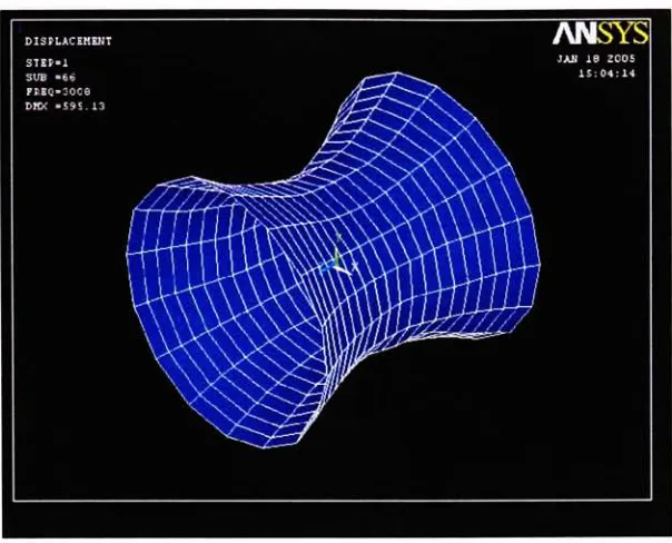
Figure 2.1 shows anexample oftheshell modeledin ANSYS. The Tables found in

Appendix Awere usedto_{quickly find}thepoints

defining

thelineandtheslopes attheend of

thespline. Thesevaluescanbetakenfromthespreadsheetandchangedwithinthebatch

Figure2.1: HSR ModelGenerated_byANSYS.

Theelement used intheANSYS analysis was Shell93. Thisisan8-Nodestructural shell

element. Eachnodehassixdegreesof

freedom,

including

bothtranslationand rotation.

According

to theANSYS _tutorial,this elementissuited for modelingcurved shells.

A preurninary studywasdoneinordertodetermine asufficient number ofelementstomesh

theHSR. It wasfoundthat 20elements_alongthelengthand 16circumferential elements

weresufficienttoget consistentresults, forafixed-free HSR. Forthefixed-fixed

HSR,

the

numberof elements _alongthelengthwasincreasedto30toobtain moreconsistent results.

[image:31.540.109.429.56.295.2]

Figure2.2: The ANSYS Finite Element MeshofHSR.

During

the_{study it}was alsofoundthat

R^

valuesbelow 1

inch,

forthefixed-free

HSR,

and

values of

Rmin

below 1.25

inches,

forthefixed-fixed

HSR,

gaveinconsistentresults.

Refining

the mesh, and/or

defining

a_completelynew mesh resultedin veryrandomresults

andmodeshapes wereunclear. Thiscouldbe dueto_{coupling between}modes and/orthe

increaseof_curvature,orthat the element used could nothandlethehighcurvature. Atrend

canstillbe foundwhenreviewingthe finalresults oftheANSYSstudy.

A dynamic studywasperformedontheHSRinANSYS. Thefirst

bending, longitudinal,

and

torsionalnaturalfrequencies forthefixed-free HSRandthe first

bending frequency

forthe [image:32.540.119.421.55.299.2]

Acylinderoflengthand_radius, 6inchesand 3 inches_{respectively,}was simulated in

ANSYS. The Batchfilecanbe found in_{Appendix B. This}wasdonetoinvestigatewhether

or nottheHSRresults were_convergingto theresultsofa cylinderwithan

increasing

Rmin. It

was foundthat theHSRresultsdid indeedconvergetoa cylinderwith

increasing

Rmin,

as shown

by

the

following

results.

2.2

RESULTS

2.2.1

DYNAMIC RESULTS

Below,

inFigures2.3 and

2.4,

arethefixed-freeHSR ANSYSresults. Figure 2.3 showsthe

naturalfrequenciesversustheratio c/d(c=

Rmin),

whileFigure 2.4showsthenatural

frequenciesversusthe minimum radius. An

increasing

c/d in Figure 2.3 correspondsto the

decreasing

Rmin

ofFigure2.4. 90UU [image:33.540.64.482.397.680.2]

>> u c

3

O"

0) 9000

8500

8000

7500

7000

6500

6000

5500

5000

4500

4000

3500

3300

2500

2000

1500

1000

500

0

First

Bendng

First Torsional

RrstLcngjtudnal

0 0.25 0.5 0.75 1.25 1.5 1.75

Mnimm Radius_(in)

[image:34.540.77.476.63.357.2]

225 25 275

Figure 2.4: Minimum Radiusvs._Frequencyfor Fixed-Free HSR (ANSYS).

Itwas expectedthat as

Rmin

decreased (andc/d

increased),

theHSRwouldbecome less_stiff, andthenatural

frequency

would decrease. Thispatternisdemonstrated only forthe torsional

[image:35.540.70.494.235.517.2]

Figure 2.5 showsthefundamental

bending frequency

_{of afixed-fixed}

HSR,

_{from ANSYS.}

Consistentresults were_onlyobtained_upto

IU,

of1.25inches. Theresultsdemonstratean

increasing

natural

frequency

with

decreasing

Rmin- Contrastto thefixed-freeresults (Figure

2.4)

the

bending

natural

frequency

doesnotdecreasewith

decreasing

Rmin-12000

10000

0 0.25 0.5 0.75 1 1.25 1.5 1.75 2 2.25 2.5 2.75

Rmin(in)

2.2.2 STATIC RESULTS

Astatic _studyofthe fixed-freeHSRwas also performed. Fromthestaticanalysis the

stiffnessofthe_coupling as afunction

Rmin

was

found,

which wouldbe helpful forthedesign

ofthe_{integrated shaft-coupling}unit. Three cases were set_upto findthe

bending,

_axial, and

torsionalstiffness ofthe HSR. Batchfilescanbe found inAppendix B thatcanbeusedto

findthestiffness ofaHSR. Figures

2.6,

2.7and2.8showthe

Bending

Stiffness,

Torsional

StiffnessandAxial Stiffnessas

functions

of

Rmm,

respectively.

1600

0 0.25 0.5 0.75 1 1.25 1.5 1.75 2 2.25 25 2.75 3

Mnimum radius(in)

[image:36.540.84.463.275.558.2]

3000

1 1.25 1.5 1.75 2

Minimumradius_(in)

Figure2.7:Minimum Radiusvs.TorsionalStiffness.

35000

30000

0.25 0.5 0.75 1.25 1.5 1.75

[image:37.540.51.490.61.316.2]

Minimum Radius_(in)

[image:37.540.53.481.77.634.2]

Thetrendsofthestiffness plots(Figures

2.6, 2.7,

and

2.8)

are similarto their_{corresponding}

natural

frequency

trends (Figure 2.4). Boththe

bending

and axial

stiffness'

initially

increase

with

decreasing

Rmin,

followed

by

adecreaseinthefrequencies. Similarto the torsional

CHAPTER

3: TIMOSHENKO BEAM

THEORY

3.1

MATHEMATICAL MODEL

The HSRwasfurtherstudied

by

means ofbeamtheory. Inordertoconsiderbothshear and

bending,

theTimoshenko beam

theory

was utilized. Thisisincontrastto the Euler-Bernoulli

beam

theory

thatneglectsshear_strain,and assumesthecross-section remains plane and

perpendicularto thelongitudinalaxis

during bending

[20].

According

toTimoshenko's

theory

thecross-sectionremains planebut doesnotremain normaltotheaxis. Theshear

angle, y,isthedifference betweenthe angleto thenormalofthe cross-section, (|),andthe

slope of_{the centerline,} dw/dx (Figure 3.1).

Figure 3.1:TimoshenkoBeamDifferentialElement

Two equations ofmotion, onefortransversetranslation, w, andoneforrotation, <f>, were

writtenfromthe Timoshenkobeamdifferentialelement (Figure 3.1). Equations 3.1 and3.2

aretheequationsofmotionintermsof_{the shear,}

V,

andmoment,M.

V'

= -pAw.

C3-1)

Themomentandtheshear werefound fromthe elastic equation ofthebeamand are given

by

Equations 3.3 and3.4.

M=EI^-,

dx

And

(3.3)

(

dw\

V =

kGAy

=

kGA\0-I

dx

(3.4)

Theconstantk istheTimoshenkoshear_coefficient, G istheshear_modulus,E is Young's

Modulus,

A isthe area, andI isthemoment ofinertia. Theshear coefficientvaries

depending

ontheshape ofthecross-section. Thisconstant isusedto accountforthe

assumption of constantshearoverthecross-section [20].

Depending

onthesource,itsvalue

canvary. Forthis thesiskwas setto .5and.9. Thisgives arangeofresultsforthenatural

frequencies.

Together,

withtheappropriate

boundary

_conditions,Equations 3.5 and

3.6,

representthemathematicalmodel oftheTimoshenkoBeam.

kGA

2...\

dip

d

w

dx

dx7

=-pAw

(3.5)

EI

a*2 kGA

</>

dw

dx

=pl<j>

(3.6)

Equations 3.5 and3.6are obtainedfrom substituting Equations 3.3 and3.4 intoEquations3.1

and

3.2,

respectively. The Equations willbesolvedforthenaturalfrequencies usingfinite

3.2

FINITE ELEMENT FORMULATION

The finiteelementformulationwasdone in foursteps:

(1)

MeshGeneration andFunction Approximation: The_{translation,w,}andthe rotation,^,

wereapproximatedby:

0

=

Y/D;.

_{and w}=

YiJWj.

(3.7)

Where

Wj

and

<E>j

arethenodaltransversedisplacementand rotationcomponents,respectively

and

Wj

istheshapefunction. The Hermitecubicinterpolation

functions,

Equation

3.8,

were

adoptedforthis analysis.

,P1(x)

=H-2

'*V

Vy

x

yhj

W2{x)

=_x-2

x2

+ h

x3

/z2'

y3{x)

=3

(-Khj

2

-2

-T

Ah)

r

.3 -A_

h

"

(3.8)

(2)

The ElementEquation: Theelement equationcanbewrittenas

[M]etA+[K]eUe=0

(3.9)

Where[M]eand [K]e

aretheelement massandstiffness matrices, respectively,and Ifis the

The shapefunctionswerefirstsubstitutedintotheequations of motiontoobtainthe

residuals,R:

Rj^V'

+_pA^VjWj,

(3.10)

And

Rj*

=

\M'-v]-/*jyj*j-(3.11)

Where

V =

kGAfEvpj

-^jWj),

(3.12)

And

M^EI^X^j-

(3.13)

Next,

theweightedresiduals wereformed

by

_multiplyingtheresiduals

by

theweight

functions,

Yj. Theweighted residualswereintegratedovertheelement and set equaltozero.

x2 x2

J

Wy'dx+

|

%/aAE

VjWdx-0 ₍₃

.

14)

xl x\

x2 x2

\Wi[M'-v}ix-$%pIZlyj<!>dx

=0

(3.15)

xl xl

Integrating

Equations 3.14and3.15

by

parts and_expandingyields:

{V,.

_{pt$y,wdx-]x zlkGA^yp;}

-y;w>=-%v\*,

0.16)

xl xl

Equations

3.16and3.17canberepresented as:

MA+(K^\jWj+(K4.^j=%V\Xx2i,

And

Jv*j+(Kj9Wj+{K\*j=VtM\".

Where:

xl

{Kww)ij=kG)%AV'jdx,

xl

xl

j(,=p\vlrjdx

xl

xl

(3.18)

(3.19)

(3.20)

xl

Inmatrix

form,

Equations 3.18 and

3.19,

are given

by

3.21. Notice_that,there are no external

forces,

moments,ormasses appliedto theshellinthis analysis;therefore,theforcevectoris

settoall zeros.

[m]

[o]ljw

to]

urn1

[Kwp]

[Kpp]

w[_

0}

InEquation

3.21,

Wisthenodaltransversedisplacementvector{W=

[Wj, Wj

',

W2,

W2']1)

andO isthenodal angular rotation vector(O=

[O], O/,

<2,

O2']1),

where a prime denotes

thefirst derivativewith respecttox.

Notethatupon_performingtheintegrationinEquation

3.21,

AandIare consideredfunctions

oftheaxial global coordinate X:

A{X)

=

x(r0{X)2-ri{X)2)

and

I{X)

=^(r0{X)4

-r,{X)4}

(3.22)

Whereglobal coordinateX is afunctionoflocal element_coordinate, x:

X=X0+x,

(3.23)

andXoistheglobalcoordinate oftheelement coordinate xl (atnode 1).

(3)

Assembly

oftheGlobal Equation:

Assembly

ofthelocalelement equationsintothe

globalequationwas done

by

_usingthestandardfiniteelement_assemblymethod

[32],

rendering:

[MY[

+

[Kll

=0

(3.24)

Where

[M]

and

[K]

arethe assembled globalmass and stiffness _{matrices, respectively,}and U

istheglobal nodal displacementvector. Programs werewritteninMatlabtoassemblethe

global equationforthefixed-freeandfixed-fixed

boundary

conditions (Appendix C).

(4)

Solving

fortheEigenvalues: A Matlabprogramwaswrittentoobtaintheeigenvalues and

3.3

RESULTS

Figures 3.2and3.3 aretheresults forafixed-freeandfixed-fixed

HSR,

respectively. The

resultswereobtained

by

_applyingfiniteelements totheTimoshenkomathematicalmodel

withtheappropriate

boundary

conditions.

Forthefixedends:

w=

^

=<Z>=

0,

(3.25)

dx

And forthefreeend:

kAG

\

dw

-0

ox

=7-^=0.

(3.26)

dx

In Appendix CtheMatlab M-filesusedtofindthenatural_{frequencies for varying}

Rmin

can

Figure3.2 showsthe

bending

natural

frequencies,

forthefixed-free

HSR,

versusRmi. Plots

are givenfortheshear

factor,

k,

equalto .5 and.9. Theresults show a

decreasing

_natural

frequency

with

decreasing

R^n- As expectedthenatural

frequency

_{increaseswith an}

increaseofk. Notethat thecurvesforthe

different

shear coefficients seemto convergewith

decreasing

Rmin.

4000

Rmin_(in)

[image:46.540.54.459.222.491.2]

Figure 3.3 showsthe

bending

natural

frequencies,

_{forthefixed-fixed}

HSR,

_versusthe

minimum radius.

Again,

plots are givenfortheshear

factor,

k,

equalto .5and.9. The

results showthat as

Rmin decreases

_thenatural

frequency

increases.

Again,

thehighershear

coefficient resultsinhighernatural

frequencies.

_Notice

that,

_{contrastto thefixed-freeresults}

(Figure

3.2)

the two curves(k=

.5andk

=

.9)divergeas

R^n

decreases.

16000

14000

2.25 2.5 2.75 0.25 0.5 0.75 1 1.25 1.5 1.75 2

Rmin_(in)

[image:47.540.65.491.227.500.2]

Chapter

4:

SHELL THEORY

4.1

MATHEMATICAL

MODEL

4.1.1 KIRCHOFF-LOVE THEORY OF SHELLS

During

thesecondhalfofthe 19th

Century

Loveadded assumptionstoKirchoff's

assumptions forthe

theory

of plates sothatitcouldbeextendedtothe

theory

ofshells. This

is sometimes calledtheKirchoff-Love

Theory

ofShellsorjust Love's

Theory

ofShells.

Later Reissneraddedtheinfluenceoftransverse shear strainstothe

theory

of shellsto

providemore accurate solutions.

Many

othershavecontributedto themechanicsof shells of

revolution

including

butnotlimitedto:

Timoshenko,

Girkann, Novozhilov, Vlasov, Lur'e,

andKrauss [10].

Thebasic approachofshell

theory

istoreplace3-dimensional analysis

by

theanalysis of

hypothetical 2-dimensions. The kinematics andthekineticsare_normallyreferredto the

middle surface oftheshell. Thispremiseformsthefoundationofthelinearclassical shell

theory

[5].

Fourmain assumptionswere made

by

Love,

andhereferredto themashis "first

approximation"

shell theory.

(1)

Theshellthicknessissmall compared withthesmallest radius of curvature ofthe

middlesurface oftheshell.

(3)

Normal stresses,transverse tothemiddle_surface,are small when compared with

other_stresses, and canbeneglected.

(4)

Normalstothemiddle surface oftheshell will remain normal to themiddle

surfaceinalldeformedconfigurations of_{the shell,} andwill notbesubjectto

deformation.

Thefirstassumptionisthebasisforallthinshell

theory

[14]. Thethicknessoftheshell

shouldbeseveraltimeslessthen theradiiofthe shell as well as otherdimensions

describing

theshell.

According

toNovozhilov

[10],

the_{relationship h/R}< 1/20shouldbesatisfiedin

ordertoachieve errors of5%or

less,

where

'h'

is theshellthickness and 'R'

is thesmallest

radius oftheshell. The fourthassumptionis Kirchhoff's hypothesis.

According

to this

assumptionthestrainsinthedirectionnormaltothe shell arezero. This greatly simplifies

thedevelopmentofthe

theory

[10].

4.1.2

MATHEMATICAL MODEL OF A SHELL

OF REVOLUTION

Themathematicalmodel of ashell ofrevolutionis developed basedontheclassical

mechanics approach. Theequilibrium equationsaredevelopedasfunctionsofforcesand

displacements.

Substituting

theconstitutive equations (stress-strainrelationships) andthe

straindisplacementrelationships

(Kinematics)

into theforceequations, themathematical

4.1.2.A

KINEMATICS

Therelationships ofthedisplacementsto the _{strains, eamdco, the}changes in_{curvature, %0}

andthe_twist,x, can bewritten as [10]:

1

du

1

^o^V^-^'

z

=

1

(dv

" w

dtp

R,

J

1 dv 1

du

u

OJ=

-+ _cos<p,

R0

d&

R2

dtp

R0

Zi=~

1

R

'dX,

o V

d&

+

X2

cos_<p ,

z2=-1

dX2

R2

dtp

'

T=

R_{o V}

dx2

d&

-X1

cos_cp

1

du

RYR2

dtp

wheretherotations,

Xa

,aregiven as:

1

dw

u

X,

= ₊

, Rod*

R!

X,

_\_

R,

dw

dtp

\ +v

(4.1)

(4.2)

Whereu isthecircumferential

displacement,

vis thedisplacementtangenttothemeridian ,w

isthe transversedisplacementnormaltothe surface, andthe radii,

R0, Ri,

and

R2

(Figure

4.1)

arethe distancenormal fromthecenter axistothe meridian, theradiusof circumferential

~~

"

A^SSfisr^^v

Figure4.1:CoordinatesofShell [10].

[image:51.540.133.419.56.218.2]

4.1.2.B

CONSTITUTIVE RELATIONSHIPS

Figure 4.2shows adifferential elementforashell, withthestress components _actingacross

the thicknessofthe shell.

Notice,

_accordingtoLove's assumptionsthestresses normal to the

middle surface are neglected.

[image:51.540.118.425.459.612.2]

Hooke's

Lawgives thestress-strain relationships. In threedimensions Hooke's Law canbe

written as:

fi=-k

-^2+o-3)l

E

2=

fa-vfa+vjl

3

=-[^3-^1+^)1

(4.5)

07

12

G

a -g21

21 ,-,

Ca3 ^

whereEis Young's

Modulus,

G istheShear

Modulus,

and visPoisson'sratio.

Considering

Love'sthirdand_{fourth assumptions^} =

eu

=

f23

=

cr13 =cr23 =

<73 =0,

Hooke's lawreducesto:

E

(4.6)

<-2

E 2

e3--=

0,

u

"l2

G

'

2\

21

G

'

a3

=_0.

Equation4.6canbepresentedina morecondensedform as:

(ra=

Where:

V =₃

-a, with a =_{\ and a}=_2.

(4.8)

4.1.2.C FORCE AND MOMENT

EXPANSION

[image:53.540.127.436.231.384.2] [image:53.540.55.179.512.698.2]

Theunitforces and moments_actingonthefacesofthedifferentialelementare shownin

Figure 4.3.

Figure 4.3: Unit_{Forces,Moments,}andTorques_Actingonthe DifferentialElement

Theforces

N, Nav,

and

Qa

arethenormal, shearandtransverseforces_{respectively;} while

momentsandtorques are

Ma,

andMav-

They

aredefinedper unitlengthand arefound

by

integrating

thestress overthe thicknessoftheshell.

A/2

Na=

\(Ta(l-zKv)dz,

-h/2

A/2

Wov=

j

^ov(l-zKv)dz,

-A/2

Qa=

\crJ\-zKv)dz,

(4-9)

-A/2 A/2

Ma=

\(ya{l-zKv)zdz,

-A/2 A/2

M^=

\cry\-zKv)zdz.

Where

ATV

is thecurvaturesdefinedas

Kv

=1/_R

V

Considering

Love'sthirdassumption

(o"b

=

a23=

0),

Equation 4.9_sets

Qa

=0.

However,

Qa

isnot assumedtobezeroand willbesolvedfor later usingtheequilibrium equations.

Carrying

outtheintegrationofEquation 4.9and_{neglecting higher}order_terms,thefinalunit

force,

moments, andtorquesexpressedintermsof strain components are:

Na=C{a+Vvv),

Nl2

=

N21

=

CnOJ,

Ma=D{xa+vvv),

Ml2

=

M21

=D12T.

Where:

D=

Eh3

C=

Eh

l-v2

'

And

A2=-Gh

12'

(4.10)

Cl2=G12h,

(4.11)

12

2(1+

where

Gn

istheshear modulus.

4.1.2.D

EQUILIBRIUM

EQUATIONS

Fromthedynamicequilibrium ofthe

differential

element(Figure

4.3)

the equilibrium

equationscan bedefinedas

[10,

_31]:

_

dNx

d(R0N2i)

2

"a*

+

dV

+ 2"n cos*

"

/?2Gi

sin_?+

RR^

=

a

_

diV12

d{R0N2)

2^f+

d^

"

RlNl

CS_*"

*fi*

+

*0^

=

'

_

aa

a(/?0<22)

Rl

m

+

d^

+

*2Nl

sm_*+

* ^2

+

****&

=

'

dAf,

3(i?0M21)

2"5^+

dp

+^M2Cos^-J?0J?2gl+JR0/?2/4=o,

3M12

a(/?0M2)

2~a#+

aV

RiMicos<p-RoR2Q2+R0R2f5

=o,

*2

*,

Thevalues of

f,

in Equation

4.13,

are given

by

Equation 4.14 [10].

d'u

.

,

du

d2w

.

,

a>v

/i

=Pi-ph^r-Alh -kiu>

fi

=

P2

-Ph^T-^h-2v>

(4.13)

f3

=

P3 -ph-TT-Aih-k3w,

(4.14)

, h3

a2x,

h3

dx,

h=Pn~dtr^n~dT'

, /i3

a2z2

&3

ax2

/5=_/?T2""a7^+/l2L2""ar-Where

/j

arethe_auxiliary

forces,

pirepresentstheloadonthe shell,

&,

are coefficients

describing

the_elasticityof aWinkler-type_subgrade, and

A,;

representthe

damping

coefficient

ignored

kt,

andhadno external loads applied_{to the shell; therefore,}thevalues of

f

_simplify

to:

d2u

fi

=_-fih

f2

=_~ph

dt2'

v

a2-dt2'

r 7

d2

,a ,n

f3=~PhWT>

(4-15)

a?

/i3

a2x,

/4=/o

fs=-P

12 a?2

'

/i3

a2z,

12 a?2

Inthis

formfj,f2,

and/3arethelinear inertia forcesoftheshellin the u,vandw

directions,

respectively, andthevalues of

f\

and/5representthe_{rotary inertia}oftheshell.

Thesixth equilibriumequation_maynot_{exactly be}satisfiedfora

doubly

curvedshell. To

avoidthis

inconsistency

Novozhilovusedan_energymethodtoexpress

N]2

and

N2i

as [10]:

Nl2

=_Cl2OJ

-D12K2T,

and

(4.16)

N2l=Cl2a)-DllKiT.

A derivationoftheserelationships (Equation

4.16)

is given

by

Leissa [14]. These

relationships willbeusedinthedevelopmentoftheHSR's equations of_motion,asdone

by

4.1.3

MATHEMATICAL

MODEL OF THE

HYPERBOLOID

SHELL

OF

REVOLUTION

Thedevelopedapproach oftheequilibrium equation ofChapter 4. 1.2is adaptedand applied

to thedevelopmentofthemathematical model oftheHSR. Three-coupledequation of

motionaredeveloped fromtheequilibrium equations andpresentedinmatrixform.

4.1.3.A

KINEMATICS

Considering

theEquationof a

hyperbola,

twodimensionlesscoordinates weredefinedas:

=

4,

_*=

?*-,

(4-18)

d c

which changedtheEquation of ahyperbolato:

//2-f=l.

(4-19)

Using

the threerelationships:

The

following

relationshipswere verified[10]:

dR^_

dji

d2R0

=

A2

d2rj

d'

dz2 c

d2 '

R\

-CC>

R2

-12 2

1

a

Arj

a

_?]

A

=

-, sin#? =

,

R

dip

cCd

C

drj

d

n

d2rj

1

d{2

KG

=

KlK2

-A2

c2C^

cos<p= ,

A%

cotcp=

^--

= _-*!_. K,=K,K,-4^r,

(4-21)

It is importantto note,inthecaseofa

HSR,

that

R2

isnegative. Forthisreasonexact

analyticalsolutionsareconsidereddifficulttoobtain [10].

Substituting

Equations 4.20and4.21 into Equations 4.1 and

4.2,

thestrain-displacement

relationshipsoftheHSRwereverifiedtobe:

*!=

1

f

du

An + -v

d&

c

CTJ

An

3v

Aw

f = - ₁

2 _y i e _/-3

' w

cdt cC

OJ= _1_

en

d\

Ag \

An

du

u

d$

c

+

Zi

=

Xi=-^4x

d&

C

cCdf

T=

cn

An

dX2

i

fax2

At

cn

d&

X,

An

du

AC2"^'

(4.22)

wherethe rotations,

Xa,

are:

*i

=

*2

=

cn

An

dw

n

+_u

dw

A

d

riC

4.1.3.B

EQULILIBRIUM

EQUATIONS

Considering

Equations

4.10, 4.16,

and4.21 theunit

forces,

moments, andtorquesbecome

(They

canbe foundintheirexpandedform in Appendix D):

Na=C{a+Vv),

N₁₂

C(l

s

D{\-v)A2

=_-(l-V>+ V >

T,

2 _cQ

N2i=^{l-v)co-^Ar,

(4.24)

2 _cQ

Ma=D(za+vzv),

Af12=Af21=D(l-v)r.

Substituting

Equations 4.20 and4.21 into Equation4.13 thesixequilibrium equations forthe

HSRwere verifiedtobe [10]:

d&

c

a<r

<r

t

^3-^iV

+

^-Q

_+cnf =0

d&

c

^

c

n

c

2 2

d&

,

And{nQ2)

n

A2n

(4.25)

_ci_

:2v^v^2/

j_N

-'-UJ-n _+Cnf3=0,

d&

c

^

c

c3

^+^^+KMi2-CJ?Qi+cr}fi=o,

d&

dt,

Q

M91

M,2

N12-N2l+2L r^=

0,

R2

Ri

wherethevariables/are given

by

Equations

4.15,

and

No, Nn, N2i, Ma, M12

and

M2i

are

Aswas_{previouslymentioned,}thetransverseforces

Qa

were not assumedtobeequaltozero.

They

werefoundfromthefourthandfifthequations ofEquation 4.25.

ft4(^i&)4Ml+/4i

Q2

=

cn{d&

d

C

1

\dMl2

And{nM2)

A

(4.26)

17

1

d&

+

C

d

C

~MA+

f5,

where

f4

and

f5

arefrom Equation

4.15,

andtheunit

forces,

_moments, andtorquesare given

by

Equation 4.24.

The transverseforces (Equation

4.26)

werethen substitutedintothefirstthreeequilibrium

equations;_renderingthe

following

threecoupled equations of motion:

dN,

And{nN2x)

i

1

jjM,

An

d{nM2l)

A

de

H

C

_c

d&

d

dN12

₊

And{nN2)

A%

A1

dMl2

A3nd(nM2)

A3%

^-Nl + + 4

m1+/;=o,

"x1 '

J 2

de

c

^

C

_cC

^e

_cC

d#

_cC

1

d2M1

A

d2{nM2)

A^_

dMl2

And2Ml2

A2n

d

(nd{nM2)

cn d&2 _cC

d@$

_cn

de

Cc

d@e

_cC

d{C

a<f

,3-N2+f3'=0,

A2v(^A.V,T

*2n

cC{C

M,

Vb J

+^-Nx

Where:

/i*

=crfi-^f,,

A2n

fi

=77-/5 +c7Zf2,

..

a(/4),^

a

a*

+tl^(^)+^

(4.28)

Thethree-coupledequations of motion (Equation

4.27)

canbewritten as:

^(Lnu

+Li2v+

Li3w+f;)

=₀ i=\

or

Mu Ml2

Ml3

M2l M22

M23

M3l M32

M33

y+

Lu A

2

L13

W

L2i

22 ^23 V

L31

^32

L33.

W

=0.

(4.29)

(4.30)

where

Mtj

isconstructed

from/

. Theexpanded expressionsfor

Mi}

and

Ly

arefound in

Appendix E.

The mathematical model(Equation

4.30)

canbeexpressedin a condensedformas:

|m/

+

[l]/=0,

(4.31)

Where U =_{[u v} w]T

4.2

SOLUTION

Theequationsof motion are solvedforthenatural

frequency

_usingtheAssumed Mode Shape Method.

First,

an overview oftheGalerkin

Assumed

_{ModeShape Method is}

given;followed

by

theapplicationofthemethodto theHSR.

4.2.1

INTRODUCTION

TO THE

GALERKIN

ASSUMED MODE

SHAPE METHOD

The Galerkin Assumed Mode Shape Method isusedtoapproximate solutions ofdifferential

equations.

Specifically,

_{it is a method of weighted}

residuals,wheretheweightfunctionsare

equaltothe assumed mode shapefunctions.

Considering

the

following

_equation;whereL is

adifferentialoperator_actingonthevariable_u, and/is aknown function.

L{u)

=

f

.

(4.32)

Thevariable uis approximated

by

theexpression:

ui=iyPr

(4-33)

where

*Fj

is an approximate solutionthatsatisfiesthe

boundary

conditionsofEquation 4.32.

Substitutionoftheapproximationof_Wjinto Equation 4.32producesthe _residual,R.

L(uj)-f

=R

(4.34)

It isrequiredthattheresidualbezero overthedomain. Inorderto_{satisfythis condition, the}

weighted-residualis

formed,

integratedoverthedomainand setequaltozero as shown

by

4.2.2

APPLICATION

OF THE

GALERKIN

ASSUMED

MODE SHAPE

METHOD

TO THE

HYPERBOLOID

SHELL

OF

REVOLUTOION

Inorderto_applythe _{Galerkin Assumed Mode Shape Method}

to the

HSR,

themode shapes

hadtobeapproximatedforthe

fixed-free

and

fixed-fixed

_{HSR. Theassumed shapes ofa}

cylinder were usedto approximatetheshapes oftheHSR.

According

toLeissa

[14]

the

mode shape

functions,

_forthe 'mth' mode _shape, of a cylinder canbeapproximatedby:

Vum=Xm{z)Sin{ne),

Vvm=X'm{z)Cos{ne),

(436)

VZ=Xm{z)Cos(nr),

where

Xm{z)

isthemode shape ofthe lateralvibration ofa

beam,

andthe_{corresponding}

coordinate ofthe shape

function, Tm,

is given

by

itssuperscript. Itwasknown

approximatingthemode shapes oftheHSR

by

the mode shapefunctionsofa_cylinder,

Equation

4.36,

introducederror.

Themode shape of a_{lateral vibrating beam is}givenby:

Xm {z)

=

C,

cos_j3mz+

C2

sin

/3mz

+

C3

cosh

/3mz

+

C4

sinj3mz,

(4.37)

where

Ci, C2, C3,

and

C4

are constantsfound

by

_applyingtheappropriate

boundary

conditions and

fim

isaparameterproportionalto thenatural

frequency

anddependsonthe

boundary

conditions:

1

(4.38)

,

(El\

Pm

=Jam

Boththefixed-freeandfixed-fixed beam'smode shapeswerefound usingtheappropriate

boundary

conditions.

Forafixedend:

dX

Xm=0,

and ^=_0.

(4.39)

oz

Forafreeendthe

bending

moment and shear areboth_zero;therefore:

r)2Y f)3Y

^-^

=

0,

_and

^rf-

=0.

(4-40)

dz

dz

Forboththefixed-free andfixed-fixed beamtheapproximate mode shapeis:

Xm{z)

=sin/3mz-smhj3mz-am{cosj3mz-cosh/3mz).

(4.41)

Forafixed-free beam:

_

smfij+sinhfij

(442)

m

cos

0J

+cosh

0J'

with

fixl

=_{1.875 104 forthe}firstnaturalfrequency.

Forafixed-fixed beam:

_

sinh/?m/-sinlm/

(443)

m

cos

fij

-cosh

fij'

The

displacements

werethen approximated as:

u =_Y:u =_{Xm{z)Sin{ne)U}

v =_x:v =

X'm{z)Cos{ne)V,

w=yw=

Xm

{z)Cos{ne)W,

(4.44)

where

XJz)

isforafixed-freeorfixed-fixed

beam,

andforthe

HSR,

uisthecircumferential

displacement,

visthedisplacementtangent tothe meridian andwisthe transverse [image:65.540.199.341.235.344.2]

displacementnormal_{to the surface,} as shown

by

Figure 4.4.

Figure 4.4: Displacementcoordinatesfor the HSR.

The displacementapproximations werethenwrittenintermsofthevariables _<fand

d,

by

substituting z=

d

into

Xm{z)

_and

X'ffl(z),

andthenintothe threeequationsofmotion

(Equation

4.30);

_renderingtheresiduals:

l1{w:u,w:v,w:w}+m1{^:u,w:v,^:w}^r1,

L2{w:u,w:v,w:w}+M2{v:u,v;v,vm'w}=R2,

<